The Thirty-Third AAAI Conference on Artificial Intelligence (AAAI-19)
Recurrent Poisson Process Unit for Speech Recognition
Hengguan Huang,
1Hao Wang,
2Brian Mak
1 1The Hong Kong University of Science and Technology2Massachusetts Institute of Technology {hhuangaj,mak}@cse.ust.hk,[email protected]
Abstract
Over the past few years, there has been a resurgence of interest in using recurrent neural network-hidden Markov model (RNN-HMM) for automatic speech recognition (ASR). Some modern recurrent network models, such as long short-term memory (LSTM) and simple recurrent unit (SRU), have demonstrated promising results on this task. Recently, sev-eral scientific perspectives in the fields of neuroethology and speech production suggest that human speech signals may be represented in discrete point patterns involving acoustic events in the speech signal. Based on this hypothesis, it may pose some challenges for RNN-HMM acoustic modeling: firstly, it arbitrarily discretizes the continuous input into the interval fea-tures at a fixed frame rate, which may introduce discretization errors; secondly, the occurrences of such acoustic events are unknown. Furthermore, the training targets of RNN-HMM are obtained from other (inferior) models, giving rise to misalign-ments. In this paper, we propose a recurrent Poisson process (RPP) which can be seen as a collection of Poisson processes at a series of time intervals in which the intensity evolves ac-cording to the RNN hidden states that encode the history of the acoustic signal. It aims at allocating the latent acoustic events in continuous time. Such events are efficiently drawn from the RPP using a sampling-free solution in an analytic form. The speech signal containing latent acoustic events is recon-structed/sampled dynamically from the discretized acoustic features using linear interpolation, in which the weight param-eters are estimated from the onset of these events. The above processes are further integrated into an SRU, forming our final model, called recurrent Poisson process unit (RPPU). Experi-mental evaluations on ASR tasks including ChiME-2, WSJ0 and WSJ0&1 demonstrate the effectiveness and benefits of the RPPU. For example, it achieves a relative WER reduction of 10.7% over state-of-the-art models on WSJ0.
Introduction
Recently, recurrent neural network (RNN) has been success-fully applied to diverse machine learning problems such as automatic speech recognition (ASR) (Graves, r. Mohamed, and Hinton 2013), machine translation (Bahdanau, Cho, and Bengio 2015) and computer vision (Vinyals et al. 2015). Al-though end-to-end encoder-decoder approaches are getting more popular in ASR, the hybrid long short-term memory
Copyright c2019, Association for the Advancement of Artificial Intelligence (www.aaai.org). All rights reserved.
recurrent neural network hidden Markov model (LSTM RNN-HMM) is still the dominant model used in industry (Yu and Li 2018). It is beneficial for an acoustic model to capture long-term dependencies of the observations at different times. However, the sequential gates computation of LSTM limits its parallelization potential. Simple recurrent unit (Lei and Zhang 2017) and quasi-RNN (Bradbury et al. 2016), sim-plify the implementation of LSTM-RNN, and increase the speed of computation for each processing step by dropping the connections between the hidden states and the LSTM gates, allowing them to be computed in parallel.
The hybrid RNN-HMM in acoustic modeling is essen-tially a generalized version of a dynamic Bayesian network (DBN), which is usually characterized by discretizing the time series data and capturing the dependency of those dis-cretized items. According to the research in speech pro-duction and neuroethology, human speech signals may be encoded in point patterns involving acoustic events in the speech signal and neural spikes in the brain (Stevens 2000; Esser et al. 1997). Such points in time are referred to as acoustic event landmarks in (Stevens 2002). Based on this hypothesis, it may pose some challenges for RNN-HMM acoustic modeling: firstly, it arbitrarily discretizes the con-tinuous input into the interval features at a fixed frame rate, which may introduce discretization errors and have a negative impact on the model performance accordingly; secondly, the occurrences of such acoustic events are unknown and such data are unavailable. Further more, the training targets of RNN-HMM are usually obtained from the recognition results of other (usually inferior) DBN models and misalignments are inevitable.
the continuous signal. Major research in this area focuses on exploring the observed event data to model the underlying dynamics of the system, while our work attempts to deal with the situation where acoustic events are not available/observed even during training.
In this paper, we develop a deep probabilistic model called recurrent Poisson process unit (RPPU) to deal with the afore-mentioned problems. The hybrid ASR system under the above hypothesis can be factored into three steps:
• Allocate the training acoustic events localized in time at the HMM state level to better align with the training targets. • Reconstruct/sample a series of acoustic features from the
interval features originally sampled at a fixed frame rate from the allocated acoustic events.
• Follow the traditional ASR processing procedure using the newly reconstructed acoustic features as additional inputs.
The first step is achieved by constructing a recurrent Pois-son process (RPP), which consists of a collection of homoge-neous Poisson processes (Kingman 1992) at a series of time intervals. In the proposed point process, the intensity func-tion is determined by an RNN hidden state encoding the past history of the acoustic signal. Sampling from intensity-based models is usually performed via a thinning algorithm(Ogata 1981), which is computationally expensive. Our method is sampling-free and it provides a solution in an analytical form which ensures computational efficiency. In the second step, the better aligned acoustic features are dynamically recon-structed through a linear interpolation in which the weight parameters are estimated from the acoustic events drawn from the RPP. Finally, those estimated acoustic features are provided to an RNN as additional input to perform the HMM state prediction in a traditional way.
The objective function of RPPU is designed to strike a balance between the generation of arrival times of the la-tent acoustic events for clean training data and encoding sufficient uncertainty to capture the variability caused by the discretization errors and misalignments. Notably, RPPU can be trained with the standard backpropagation through time (BPTT) (Werbos 1990). The experiments on CHiME-2, WSJ0 and WSJ0&1 show that our new model consistently outperforms the conventional LSTM, SRU and quasi-RNNs.
Background and Related Work
Modeling acoustic HMM states with RNN
A hybrid RNN-HMM ASR system (Graves, Jaitly, and Mohamed 2013) consists of an RNN estimating posterior probabilities for HMM states of context-dependent phones conditioned on the acoustic input. Typically, for a sequence of training examples[(xt1,yt1),(xt2,yt2), ...,(xtM,ytM)]
with xti ∈ R
n, y ti ∈ R
k, for1 ≤ i ≤ M, the acoustic featurextiis given as inputs to the network, while the vector
yti denotes the ground truth and is represented by a
one-hot vector ofKcontext-dependent HMM states. It can be represented by the following two equations:
hti =Gθ(xti,hti−1) (1)
ˆ
yti =sof tmax(Wyhti+by) (2)
wherehti ∈R
rdescribes the hidden state. The first equation defines the state transition mapping, in which the hidden state
hti is a nonlinear function of the current inputxti and the
previous hidden statehti−1 andθis the parameter set ofG. Wyandbyare the weight matrix and the bias of the output layer respectively. The output mapping usually adopts the softmax function to calculate the predictionsyˆti. In this sense,
the RNN can be viewed as the “state classifier” optimized by minimizing the negative log-likelihood or cross-entropy:
−logP(Y|X) =− M
X
i=1 K
X
k=1
yti,klog ˆyti,k, (3)
where both the lengths of the input sequenceXand the target context-dependent HMM state sequenceYareM; the total number of context-dependent HMM states isKand they are usually generated by forcefully aligning the training utterance with its transcription using an inferior acoustic model such as a GMM-HMM. The ultimate goal of the hybrid ASR system is to generate the most likely words or phoneme sequence. This is done by running the Viterbi algorithm (Forney 1973) within the HMM framework.
One major limitation of hybrid acoustic modeling is that training targets are generated from a family of dynamic Bayesian network models, e.g., GMM-HMM and RNN-HMM, and the arbitrary discretization of the continuous acoustic signal could result in mis-alignments. Nonetheless, the capability of handling such uncertainty only comes from the conditional output probability density given the determin-istic transition function of a standard RNN. To effectively deal with this issue, the acoustic RNN model must be capable of approximating the arrival time of each training target and reconstructing/sampling the acoustic features dynamically based on the estimated arrival time, and this is the main focus of our model.
Poisson Process
A Poisson process is a temporal point process defined in continuous time, in which the inter-arrival times are drawn i.i.d from an exponential distribution. It has a strong renewal property that the process can probabilistically restart at each arrival time, independently of the past. This enables us to describe the probabilistic behavior of the process via the intensity function λ(t), which is a non-negative function. Within a small interval[t, t+dt], the probability of an arrival isλ(t)dt.
By considering a sequence of arrival times of acoustic landmarksL = {t1, t2, . . . , tN} sampled from a Poisson processPover an interval[0, T], we have:
L∼P(g(λ(t)) (4)
∆ti=ti−ti−1∼g(λ(t)) (5) where g is the exponential density function;∆tiis the inter-arrival time. We place the first landmark at time 0 for simplic-ity, and thust0 = 0. Given the observation of the previous landmark at timeti−1, the probability that no landmark oc-curs up to time t since ti−1isP(ti > t) = e
Rt
Then, the probability that the first landmark lies in the in-terval[ti, ti+dt]sinceti−1is computed as the product of
P(ti> t)andλ(ti)dt, leading to the corresponding density function:
fi(t) =λ(t)e
Rt
ti−1−λ(t)dt (6)
By the strong renewal property, the likelihood of the whole arrivalsLover an interval[0, T]takes the form:
P(L|λ(t)) =P(tN+1> T)× N
Y
i=1
fi(ti)
=eR0T−λ(t)dt
N
Y
n=1
λ(tn)
(7)
whereP(tN+1 > T)is the probability that no landmark is observed in the interval(tN, T]. It may not be tractable as an integral over the intensity function does not always have an analytic expression. But it is not the case for a homogeneous Poisson process with a constant intensity.
Related Work
Temporal point processes have been a principled framework for modeling phenomena on an event-by-event basis across a wide range of domains. It has originally been used for model-ing earthquakes (Hawkes 1971b; 1971a) in seismology. More recently, in social network, a Hawkes process has been used to model timing and rich features of social interactions (Zhou, Zha, and Song 2013); in human activity modeling, Poisson Processes have been applied to model the inter-arrival time of human activities (Malmgren et al. 2008).
A major limitation of these existing works is that they of-ten make strong assumptions about the generative processes of the event data, which may not be well-suited for real world problem. Therefore, most of the existing works focus on enhancing the flexibility of point process models, e.g., a non-parametric Bayesian approach of point processes have been explored in (Teh and Rao 2011); (Mei and Eisner 2017) ex-tended the multivariate Hawkes process (Hawkes 1971a) to a neurally self-modulating multivariate point process using a continuous-time LSTM. Similarly, (Du et al. 2016) proposed a model based on marked temporal point process that models the event timings and the markers with the help of an LSTM. However, these methods focus only on modeling the observ-able (not latent) events, our proposed work try to develop a framework which explicitly models acoustic events as la-tent variables, consequently producing better phoneme-level alignment and leading to better ASR performance.
The closest work to ours in ASR is (Jansen and Niyogi 2009), where an acoustic model based on marked Poisson process was proposed for a sub-task of event-based ASR. This subtask requires the speech signal to be segmented prior to acoustic modeling. Therefore, the timings of the acoustic events are provided during training and the model parameters of intensity function are learned by simply using maximum likelihood estimation (MLE). In contrast, the annotations of such acoustic events are not available in our setting; hence directly supervised learning via MLE is not applicable for our task.
Recurrent Poisson Process Unit
Problem Formulation
Let us consider a time interval[0, tN], where time is dis-cretized into N frames of duration 10ms. Given a se-quence of acoustic features X = {xt1,xt2, ...,xtN}, our
goal is to approximate a sequence of arrival times Le =
{˜t1,t˜2, . . . ,˜tN}so that a new sequence of acoustic features
e
X={˜x˜t1,x˜˜t2, ...,x˜t˜N}can be estimated which should align
better with the given targetsY ={yt1,yt2, ...,ytN}in terms
of resolution and precision, and a more robust acoustic model can be learned from these newly estimated training samples.
Recurrent Poisson Process
A recurrent Poisson process (RPP), consisting of a collection of homogeneous Poisson processes (Kingman 1992) for a series of time intervals, is a special type of temporal point process, in which the intensity function is determined by an RNN hidden state encoding the history of an acoustic sig-nal. One may be tempted to learn the temporal point process simply using maximum likelihood estimation (MLE). Unfor-tunately, the annotation of the latent acoustic events in the acoustic speech signal is not available; hence direct super-vised learning via MLE is not possible. Our RPP addresses this challenge by modeling these latent acoustic events as latent variables, which are then used as part of the generative process that is linked to the training targets.
Generate Timings for a Recurrent Poisson Process As-sume that we are given N intensities{λt1, λt2, . . . , λtN}, and
a sequence of input features{xt1−d, . . . ,xt1,xt2, . . . ,xtN},
in whichdcontext frames are padded to the left. Suppose the starting acoustic landmark is at timet1−dand it follows a ho-mogeneous Poisson process with intensityλt1at the interval
[t1−d,2t1−t1−d]which starts at timet1−dand is centered att1. We will try to obtain the time estimate˜t1of the first acoustic landmark, and then repeat the procedure to obtain the wholeLe={˜t1,t˜2, . . . ,˜tN}. To be more specific, given the(i−1)-th acoustic landmark at the estimated timet˜i−1 and an interval[˜ti−1,2ti−˜ti−1], the probability density of the next landmark being in this interval can be written as:
fi∗(t) =
fi(t)
R2ti−t˜i−1
˜
ti−1 fi(t)dt
= λtie
−λti(t−˜ti−1)
1−e−2λti(ti−˜ti−1)
. (8)
Then we can estimate the time for thei-th landmark as its expected value in following closed- form solution:
˜
ti =
Z 2ti−˜ti−1
˜ ti−1
tfi∗(t)dt
=2ti−˜ti−1+ 1
λti
− 2(ti−˜ti−1) 1−e−2λti(ti−˜ti−1)
(9)
Generally, the aforementioned point process can be factored into N independent homogeneous Poisson processes. For the
i-th sub-process with intensityλti, the arrival sub-sequence Liis drawn:
If it has only one single arrival andLi ={ti}. Then, for a sequence of observationsL={L1, L2, . . . , LN}, its likeli-hood is the following joint probability density:
P(L|λt1, λt2, . . . , λtN) =
N
Y
n=1
P(Li|λt1) (11)
where
P(Li|λt1) =λtie
−λti(ti−ti−1). (12)
Conditional Intensity Function for a Recurrent Poisson Process In the neural spiking modelling (Snoek, Zemel, and Adams 2013), the intensity function of the neural spikes is usually conditioned on the external covariate. In a similar spirit, we determine our intensity function using the hidden state˜htiof an RNN, which encodes the temporal
dependen-cies among the past history of the acoustic signalX. To avoid the explosion of λ1
ti, we define the inverse of the intensity
function as:
1
λti
=cσ(φ(˜hti)) + (13)
such that the inverse of the intensity function is upper bounded bycand the intensity function is upper bounded by 1. This is important as it limits the search space during optimization whenφ(·)are neural networks, which transform the hidden states into a scalar.
Recurrent Poisson Process Unit: Integrate
Recurrent Poisson Process into RNN
The arrival time sequence of the acoustic landmarks gen-erated from a recurrent Poisson process is on the real line. However, we are only given the discretized input sequence. The missing input vectors are reconstructed by linear interpo-lation as follows:
e xt˜i=
N
X
n=1
xtnmax(0,1− |˜ti−n|). (14)
This enables the loss gradients to reach both the inputs and the estimated arrival times from the recurrent Poisson process.
In this paper, we use simple recurrent unit (Lei and Zhang 2017) to implement RNN. SRU simplifies the architecture of LSTM and dramatically reduces the computational time by dropping the connections between its hidden states and gates so that computation at the gates can be done in parallel.
Below are the updating formulas of recurrent Poisson pro-cess unit.
h
ˆ
rti,ˆfti,bcti
i
=Wx
xti,x˜˜ti
+b (15)
rti =σ( ˆrti) (16)
fti =σ( ˆfti) (17)
cti=fticti−1+ (1−fti)ˆcti (18)
hti =rtitanh(cti) + (1−rti)Wh
xti,x˜˜ti
(19)
whererti are the reset gate outputs;fti are the forget gate
outputs;cti are the memory cell outputs;WxandWhare
the weight matrices;bare the gate bias vectors;htiare the
hidden state outputs; any quantity with a ‘hat’ (e.g.,bcti) is the
activation value of the quantity before an activation function is applied;is the element-wise multiplication operation;σ
is the sigmoid function.
Learning
Our design of the loss function aims at striking a balance between the generation of arrival times of the latent acoustic events for clean training data and encoding sufficient uncer-tainty to capture the variability caused by the discretization errors and misalignments.
We use the standard Poisson process as the prior for the recurrent Poisson process to restrict the complexity of the approximated recurrent Poisson process. We measure the dis-tance between the recurrent poisson process and the standard Poisson process by Kullback–Leibler divergence in terms of the inter-arrival time distribution. The inter-arrival time dis-tribution for thei-th sub-process is defined as an exponential distributiong(λti). Since all these distributions are
indepen-dent, we can enjoy the additive property of KL divergence of these two processes:
N
X
i=1
KL(gs(λ= 1)||g(λti)) =
N
X
i=1
(λti−log(λti)−1)
(20) wheregs(λ= 1)is the inter-arrival time distribution for a standard Poisson process.
Although we assume the original arrival times of land-marks,{1,2, . . . , N}, are noisy, the negative likelihood of this “incorrect” time sequence can be a desirable regularizer to avoid overfitting in noisy conditions.
As such, the total loss is the sum of the cross-entropy loss, negative log likelihood of noisy arrival time and the KL divergence between the underlying recurrent Poisson process and the standard process:
−logP(Y|X)−αlog(P(L|λt1, λt2, . . . , λtN))
+β
N
X
i=1
KL(gs(λ= 1)||g(λti)))
(21)
Since the negative log likelihood terms and the KL terms has exactly the same form in term of optimization. The final objective can be written as:
−logP(Y|X) +γ
N
X
i=1
(λti−log(λti)) (22)
whereγis the weight for the regularization term. We adopt the backpropagation through time (BPTT) for joinly training both recurrent Poisson process and recurrent Poisson process Unit.
Experiments
Datasets
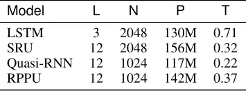
Table 1: Model Configuraions for all datasets and the training time for CHiME-2. L: number of layers; N: number of hidden states per layer; P: number of model parameters; T: Training time per epoch (hr).
Model L N P T
LSTM 3 2048 130M 0.71
SRU 12 2048 156M 0.32
Quasi-RNN 12 1024 117M 0.22 RPPU 12 1024 142M 0.37
CHiME-2 CHiME-2 corpus is a medium-large vocabulary corpus, which was generated by convolving clean Wall Street Journal (WSJ0) utterances with binaural room impulse re-sponses (BRIRs) and real background noises at signal-to-noise ratios (SNRs) in the range [-6,9] dB. The training set contains about 15 hours of speech with 7138 simulated noisy utterances. The transcriptions are based on those of the WSJ0 training set. The development and test sets contain 2460 and 1980 simulated noisy utterances, respectively. The WSJ0 text corpus, consisting of 37M words from 1.6M sentences, is used to train a trigram language model with a vocabulary size of 5k.
WSJ0 WSJ0 is a clean speech corpus recorded in a clean environment using close microphones. The standard WSJ0 si-84 training set with 7138 clean utterances was used for acoustic modeling. The evaluation was performed on eval92-5k which is a eval92-5k-vocabulary non-verbalized test set, and the si-dt-05 dataset was used as the development set. The 5k trigram language model used for evaluation was trained from the WSJ0 text corpus.
WSJ0&1 WSJ0&1 is a complete Wall Street Journal speech corpus, which involves speech data from both WSJ0 and WSJ1. The training set WSJ0&1 si-284 with 36515 ut-terances contains approximately 80 hours of speech, 95% of which was used for training. The rest was used as the devel-opment set. The evaluation of WSJ0&1 was performed on the dev93-20k and eval93-20k test sets, both of which are 20k open-vocabulary non-verbalized test sets. The evaluation was performed with a 20k trigram language model trained from the transcription of WSJ0&1 si-284. We report the speech recognition performance in terms of word error rate (WER).
Feature Extraction and Preprocessing
Acoustic hidden Markov models (HMM) based on Gaussian-mixture model (GMM), LSTM, SRU and quasi-RNN were built. GMM-HMM models employed fMLLR-adapted (Gales and others 1998) 39-dimensional MFCC features. All neural-network-based models used 40-dimensional Mel-filterbank coefficients (Biem et al. 2001) without their derivatives. In-puts of all neural networks consisted of the current frame together with its 4 right contextual frames. We performed per-speaker mean and variance normalization for the input to all the neural network models.
Table 2: WER (%) on test set of CHiME-2. Model WER
DNN Kaldi s5 29.1
LSTM 26.1
SRU 26.2
Quasi-RNN 26.1
RPPU 24.4
Training Procedure
GMM-HMM employed fMLLR-adapted 39-dimensional MFCC features and was trained using the standard Kaldi s5 recipe (Povey and others 2011). They were then used to derive the state targets for subsequent RNN training through forced alignment for ChiME-2, WSJ0 and WSJ0&1. Specifi-cally, the state targets were obtained by aligning the training data with the DNN acoustic model through the iterative pro-cedure outlined in (Dahl et al. 2012).
All RNNs were trained by optimizing the categorical cross entropy using BPTT and SGD. Prior to optimization, all the weight matrices were initialized following a LeCun Nor-mal distribution introduced in (Klambauer et al. 2017). We applied a dropout rate of 0.1 to the connections between re-current layers. The learning rate for LSTM/SRU, Quasi-RNN and RPPU models was initially set to 0.25, 0.2, and 0.07 respectively. We decayed the learning rate until it went below 1×10⁻⁶.
Models We adopted SRU as the building block to construct the proposed RPPU and compare our proposed model with the following baselines: (i) The LSTM with three stacked layers; (ii) SRU with 12 stacked layers; (iii) quasi-RNN with 12 stacked layers and the highway connection (Lei and Zhang 2017).
The LSTM has only three stacked layers because we did not observe WER reduction by stacking more layers. To ensure similar numbers of model parameters for different models, we set the number of hidden states per layer to 2048 for both LSTM and SRU, and 1024 for both quasi-RNN and RPPU. The filter width of quasi-RNN was 3, which ensured a similar number of parameters for the RPPU. Our RPPU had 2 context frames padded to the left of the input and two previous hidden states padded to the left of the input of each hidden RPPU layer. For simplicity, in the intensity function of RPPU, cwas set to 100 andwas set to 0.01 (these two hyperparameters can be tuned to further improve performance).
Results and Analysis
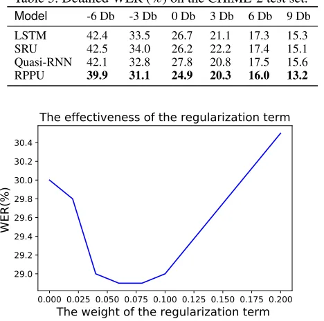
Table 3: Detailed WER (%) on the CHiME-2 test set.
Model -6 Db -3 Db 0 Db 3 Db 6 Db 9 Db LSTM 42.4 33.5 26.7 21.1 17.3 15.3
SRU 42.5 34.0 26.2 22.2 17.4 15.1
Quasi-RNN 42.1 32.8 27.8 20.8 17.5 15.6 RPPU 39.9 31.1 24.9 20.3 16.0 13.2
0.000 0.025 0.050 0.075 0.100 0.125 0.150 0.175 0.200
The weight of the regularization term
29.029.2 29.4 29.6 29.8 30.0 30.2 30.4
WER(%)
The effectiveness of the regularization term
Figure 1: WER on Development set of CHiME-2 by varying the weight of the regularization term
SRU is much faster than LSTM and our RPPU runs almost as fast as SRU while having a similar number of parameters. Table 2 shows the word recognition performance of the baseline models and the new RPPU model for CHiME-2. Firstly, we can see that all of our RNN baselines achieve a similar WER. These baselines perform much better than the DNN baseline from Kaldi s5. Our proposed RPPU per-forms the best among all the candidates in terms of WER, outperforming the RNN baselines by about 1.7% absolute. We also report the detailed WERs as a function of the SNR in CHiME-2 shown in Table 3. For all SNRs, the RPPU outperforms other models by a large margin. This suggests that incorporating the recurrent Poisson process into RNN structures lends itself to the model’s robustness.
To validate the effectiveness of the regularization term in RPPU for CHiME-2, we varied its weightγto find the best configuration, as can be seen in Figure 1. We obtained the best performance in the development set when the weightγ
is around 0.08. We hence setγto 0.08 as our final configu-ration based on this observation. These results indicate the effectiveness of our proposed objective function.
Analyze the Property of RPP Here, we took the generated time points from the recurrent Poisson process (RPP) of the 5-th layer of RPPU to perform bo5-th qualitative and quantitative analyses.
The standard Poisson process is the prior of the RPP in RPPU; hence we used the distance between the estimated value and its mean to approximately measure RPP’s flexibil-ity. To better understand how RPP works, we randomly took two utterances “423c02162” and “423c02166” at 9DB and -3DB SNR respectively, from the development set and
gener-160
162
164
166
168
Index of time steps of RPP
158
160
162
164
166
168
Estimated time points from the RPP
Plot of the estimated time points
Mean of a standard Poisson process 9DB-3DB
Figure 2: Arrival times produced by RPPU at each time steps. The yellow points represent the mean of a standard Poisson process. The blue pluses and red stars represent the generated time points estimated from the randomly chosen utterance at 9DB and -3DB SNR, respectively.
Table 4: Similarity with the ground-truth phoneme-level align-ment for our baseline and estimated alignalign-ment using RPP on development set of CHiME-2
Alignment type Similarity(%)
Baseline alignment 55.5 Estimated alignment using RPP 64.7
ated the associated arrival times from the RPP. We display the estimated time points associated with acoustic events at two different SNRs in Figure 2. We can see that as the noise level increases, the estimated time points go towards the mean of a standard Poisson process. This suggests that RPPU can pro-duce the time points based on the noise level: less flexibility is allowed for RPP’s point generation when the data is too noisy.
To evaluate how these generated time points can be helpful in better aligning the acoustic inputs with the acoustic HMM states, we conducted the analysis on the development set of CHiME-2. Notice that the noisy CHiME-2 data is generated from the clean WSJ0 data; thus the ground-truth alignments of the development set of WSJ0 serve also as the ground-truth alignments for the corresponding development set of CHiME-2 data. Here, the ground-truth phoneme-level alignment for development set of CHiME-2 is obtained by forced align-ing the development set si-dt-05 of WSJ0 usalign-ing the WSJ0 fMLLR-based DNN acoustic model.
Figure 3: In the text grids, the first tier represents the ground-truth alignment generated from the clean utterance of WSJ0. The second tier represents our baseline alignment generated from the noisy utterance of CHiME-2, and the last tier denotes the corresponding estimated alignment using RPP. The blue line and the yellow line in the middle spectrogram represents pitch and intensity, respectively.
Table 5: WER (%) on evaluation set eval92-5k of WSJ0.
Model WER
DNN (Chen and Mak 2015) 3.2
LSTM 2.8
SRU 2.8
Quasi-RNN 2.8
RPPU 2.5
alignment with such time points and then transforming it to the phoneme-level alignment. We compared it with both the ground-truth and the baseline alignment on phoneme-level to see how RPP works.
We define the similarity between two alignments by calcu-lating the percentage of their overlaps in time. The similarity with the ground-truth alignment for the baseline and the es-timated alignment using RPP are shown in Table 4. We can see that the similarity of estimated alignment achieves 9.2 % absolute gains. This demonstrates RPPU’s capability in automatically aligning the acoustic inputs with the HMM state targets.
Apart from the quantitative analysis, we show one example using Praat (Boersma and others 2002) to better understand how RPPU works. This example is the partial alignment of the randomly chosen utterance “050c01017” within the duration of the first 0.47 seconds. As shown in Figure 3, the third tier, which corresponds to the estimated alignment, is aligned much better with the ground-truth alignment shown in the first tier than the baseline alignment in the second tier. Interestingly, it seems that the first boundary in the textgrids can be determined by the intensity in the yellow line, and that the right boundary of ’F’ can be determined by the rising of the pitch. The estimated alignment fits better with the clean alignments in terms of those two boundaries. This might suggest that RPPU is capable of predicting the arrival of some acoustic events from some traits of the audio signal.
Results on WSJ0 To evaluate how RPPU behaves in a clean condition, we applied our method to WSJ0 which contains the clean utterances from which the CHiME-2
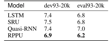
cor-Table 6: WER (%) on evaluation sets of WSJ0&1. Model dev93-20k eval93-20k
LSTM 7.4 6.8
SRU 7.5 6.8
Quasi-RNN 7.4 7.0
RPPU 6.9 6.2
pus was derived. We used the same model configurations of CHiME-2 for all RNN models. From Table 5, we can observe that all three RNN baseline systems using Mel-filterbank fea-tures achieve a WER of 2.8%. These results are comparable to the prior work using DNN (Chen and Mak 2015). Our RPPU achieves the best WER of 2.5%, yielding 10.7% rela-tive performance gain over the other RNN baseline systems.
Results on WSJ0&1 We also conducted experiments on a larger corpus, WSJ0&1. The same model configurations of CHiME-2 were applied on all RNN models in WSJ0&1. The recognition results are shown in Table 6. We can see that our best baseline LSTM achieves WER of 7.4% and 6.8% and our RPPU gives the lowest WER of 6.9% and 6.2% on dev93-20k and eval93-20k test sets, respectively. Overall, the RPPU achieves 6.8% and 9.1% relative WER reductions over the best LSTM baseline system on the two test sets.
Conclusion
We propose a novel model that can address hybrid acoustic modeling by incorporating the proposed recurrent Poisson process (RPP) into a recurrent neural network (RNN). We show that our model can generate much better alignments while performing the HMM state modeling. Our experiments on CHiME-2, WSJ0 and WSJ0&1 show that our method achieves much better results than several RNN baselines in ASR.
Acknowledgements
References
Bacry, E.; Iuga, A.; Lasnier, M.; and Lehalle, C.-A. 2015. Market impacts and the life cycle of investors orders. Market Microstructure and Liquidity1(02):1550009.
Bahdanau, D.; Cho, K.; and Bengio, Y. 2015. Neural ma-chine translation by jointly learning to align and translate.
International Conference on Learning Representations.
Biem, A.; Katagiri, S.; McDermott, E.; and Juang, B.-H. 2001. An application of discriminative feature extraction to filter-bank-based speech recognition.IEEE Transactions on Speech and Audio Processing9(2):96–110.
Boersma, P., et al. 2002. Praat, a system for doing phonetics by computer.Glot international5.
Bradbury, J.; Merity, S.; Xiong, C.; and Socher, R. 2016. Quasi-recurrent neural networks. arXiv preprint arXiv:1611.01576.
Chen, D., and Mak, B. 2015. Distinct triphone acoustic modeling using deep neural networks. Ininterspeech. Consortium, L. D., et al. 1994. CSR-II (WSJ1) complete.
Linguistic Data Consortium, Philadelphia, vol. LDC94S13A. Dahl, G. E.; Yu, D.; Deng, L.; and Acero, A. 2012. Context-dependent pre-trained deep neural networks for large-vocabulary speech recognition. IEEE Transactions on audio, speech, and language processing20(1):30–42.
Du, N.; Wang, Y.; He, N.; Sun, J.; and Song, L. 2015. Time-sensitive recommendation from recurrent user activities. In
Advances in Neural Information Processing Systems, 3492– 3500.
Du, N.; Dai, H.; Trivedi, R.; Upadhyay, U.; Gomez-Rodriguez, M.; and Song, L. 2016. Recurrent marked tem-poral point processes: Embedding event history to vector. In
SIGKDD, 1555–1564.
Esser, K.-H.; Condon, C. J.; Suga, N.; and Kanwal, J. S. 1997. Syntax processing by auditory cortical neurons in the FM–FM area of the mustached bat Pteronotus parnellii. Pro-ceedings of the National Academy of Sciences94(25):14019– 14024.
Forney, G. D. 1973. The Viterbi algorithm.Proceedings of the IEEE61(3):268–278.
Gales, M. J., et al. 1998. Maximum likelihood linear trans-formations for HMM-based speech recognition. Computer speech & language12(2):75–98.
Garofolo, J.; Graff, D.; Paul, D.; and Pallett, D. 1993. CSR-I (WSJ0) complete.Linguistic Data Consortium, Philadelphia. Graves, A.; Jaitly, N.; and Mohamed, A.-r. 2013. Hybrid speech recognition with deep bidirectional LSTM. In Pro-ceedings of the IEEE Automatic Speech Recognition and Understanding Workshop, 273–278.
Graves, A.; r. Mohamed, A.; and Hinton, G. 2013. Speech recognition with deep recurrent neural networks. In Pro-ceedings of the IEEE International Conference on Acoustics, Speech, and Signal Processing, 6645–6649.
Hawkes, A. G. 1971a. Spectra of some self-exciting and mutually exciting point processes.Biometrika58(1):83–90.
Hawkes, A. G. 1971b. Spectra of some self-exciting and mutually exciting point processes. Biometrika58(1):83–90. Jansen, A., and Niyogi, P. 2009. Point process models for event-based speech recognition. Speech Communication
51(12):1155–1168.
Kingman, J. F. C. 1992.Poisson processes, volume 3. Claren-don Press.
Klambauer, G.; Unterthiner, T.; Mayr, A.; and Hochreiter, S. 2017. Self-normalizing neural networks. InAdvances in Neural Information Processing Systems, 971–980.
Lei, T., and Zhang, Y. 2017. Training RNNs as fast as CNNs.
arXiv preprint arXiv:1709.02755.
Malmgren, R. D.; Stouffer, D. B.; Motter, A. E.; and Amaral, L. A. 2008. A Poissonian explanation for heavy tails in e-mail communication.Proceedings of the National Academy of Sciencespnas–0800332105.
Mei, H., and Eisner, J. 2017. The neural Hawkes process: A neurally self-modulating multivariate point process. InNIPS, 6757–6767.
Ogata, Y. 1981. On Lewis’ simulation method for point pro-cesses.IEEE Transactions on Information Theory27(1):23– 31.
Povey, D., et al. 2011. The Kaldi speech recognition toolkit. InProceedings of the IEEE Automatic Speech Recognition and Understanding Workshop.
Snoek, J.; Zemel, R. S.; and Adams, R. P. 2013. A determi-nantal point process latent variable model for inhibition in neural spiking data. InNIPS, 1932–1940.
Stevens, K. N. 2000. Acoustic phonetics, volume 30. MIT press.
Stevens, K. N. 2002. Toward a model for lexical access based on acoustic landmarks and distinctive features. The Journal of the Acoustical Society of America111(4):1872–1891. Teh, Y. W., and Rao, V. 2011. Gaussian process modu-lated renewal processes. InAdvances in Neural Information Processing Systems, 2474–2482.
Vincent, E.; Barker, J.; Watanabe, S.; Le Roux, J.; Nesta, F.; and Matassoni, M. 2013. The second CHiME speech separa-tion and recognisepara-tion challenge: Datasets, tasks and baselines. In Proceedings of the IEEE International Conference on Acoustics, Speech, and Signal Processing, 126–130. Vinyals, O.; Toshev, A.; Bengio, S.; and Erhan, D. 2015. Show and tell: A neural image caption generator. In Proceed-ings of the IEEE Conference on Computer Vision and Pattern Recognition.
Werbos, P. J. 1990. Backpropagation through time: what it does and how to do it.Proceedings of the IEEE78(10):1550– 1560.
Yu, D., and Li, J. 2018. Recent progresses in deep learning based acoustic models (updated). arXiv preprint arXiv:1804.09298.