Deep Optimal Stopping

Deep Optimal Stopping

Sebastian Becker [email protected]

Zenai AG, 8045 Zurich, Switzerland

Patrick Cheridito [email protected]

RiskLab, Department of Mathematics ETH Zurich, 8092 Zurich, Switzerland

Arnulf Jentzen [email protected]

SAM, Department of Mathematics ETH Zurich, 8092 Zurich, Switzerland

Editor:Jon McAuliffe

Abstract

In this paper we develop a deep learning method for optimal stopping problems which directly learns the optimal stopping rule from Monte Carlo samples. As such, it is broadly applicable in situations where the underlying randomness can efficiently be simulated. We test the approach on three problems: the pricing of a Bermudan max-call option, the pricing of a callable multi barrier reverse convertible and the problem of optimally stopping a fractional Brownian motion. In all three cases it produces very accurate results in high-dimensional situations with short computing times.

Keywords: optimal stopping, deep learning, Bermudan option, callable multi barrier reverse convertible, fractional Brownian motion

1. Introduction

We consider optimal stopping problems of the form sup_τEg(τ, Xτ), where X = (Xn)Nn=0 is anRd_{-valued discrete-time Markov process and the supremum is over all stopping times}

τ based on observations of X. Formally, this just covers situations where the stopping decision can only be made at finitely many times. But practically all relevant continuous-time stopping problems can be approximated with continuous-time-discretized versions. The Markov assumption means no loss of generality. We make it because it simplifies the presentation and many important problems already are in Markovian form. But every optimal stopping problem can be made Markov by including all relevant information from the past in the current state of X (albeit at the cost of increasing the dimension of the problem).

In theory, optimal stopping problems with finitely many stopping opportunities can be solved exactly. The optimal value is given by the smallest supermartingale that domi-nates the reward process – the so-called Snell envelope – and the smallest (largest) optimal stopping time is the first time the immediate reward dominates (exceeds) the continuation value; see, e.g., Peskir and Shiryaev (2006) or Lamberton and Lapeyre (2008). However, traditional numerical methods suffer from the curse of dimensionality. For instance, the complexity of standard tree- or lattice-based methods increases exponentially in the di-mension. For typical problems they yield good results for up to three dimensions. To

c

treat higher-dimensional problems, various Monte Carlo based have been developed over the last years. A common approach consists in estimating continuation values to either derive stopping rules or recursively approximate the Snell envelope; see, e.g., Tilley (1993), Barraquand and Martineau (1995), Carriere (1996), Longstaff and Schwartz (2001), Tsit-siklis and Van Roy (2001), Boyle et al. (2003), Broadie and Glasserman (2004), Bally et al. (2005), Kolodko and Schoenmakers (2006), Egloff et al. (2007), Berridge and Schumacher (2008), Jain and Oosterlee (2015), Belomestny et al. (2018) or Haugh and Kogan (2004) and Kohler et al. (2010), which use neural networks with one hidden layer to do this. A different strand of the literature has focused on approximating optimal exercise boundaries; see, e.g., Andersen (2000), Garc´ıa (2003) and Belomestny (2011). Based on an idea of Davis and Karatzas (1994), a dual approach was developed by Rogers (2002) and Haugh and Kogan (2004); see Jamshidian (2007) and Chen and Glasserman (2007) for a multiplicative ver-sion and Andersen and Broadie (2004), Broadie and Cao (2008), Belomestny et al. (2009), Rogers (2010), Desai et al. (2012), Belomestny (2013), Belomestny et al. (2013) and Lelong (2016) for extensions and primal-dual methods. In Sirignano and Spiliopoulos (2018) op-timal stopping problems in continuous time are treated by approximating the solutions of the corresponding free boundary PDEs with deep neural networks.

In this paper we use deep learning to approximate an optimal stopping time. Our ap-proach is related to policy optimization methods used in reinforcement learning (Sutton and Barto, 1998), deep reinforcement learning (Schulman et al., 2015; Mnih et al., 2015; Silver et al., 2016; Lillicrap et al., 2016) and the deep learning method for stochastic control problems proposed by Han and E (2016). However, optimal stopping differs from the typical control problems studied in this literature. The challenge of our approach lies in the imple-mentation of a deep learning method that can efficiently learn optimal stopping times. We do this by decomposing an optimal stopping time into a sequence of 0-1 stopping decisions and approximating them recursively with a sequence of multilayer feedforward neural net-works. We show that our neural network policies can approximate optimal stopping times to any degree of desired accuracy. A candidate optimal stopping time ˆτ can be obtained by running a stochastic gradient ascent. The corresponding expectationEg(ˆτ , Xˆτ) provides a lower bound for the optimal value supτEg(τ, Xτ). Using a version of the dual method of Rogers (2002) and Haugh and Kogan (2004), we also derive an upper bound. In all our examples, both bounds can be computed with short run times and lie close together.

motion. But fractional Brownian motion is not Markov. In fact, all of its increments are correlated. So, to optimally stop it, one has to keep track of all past movements. To make it tractable, we approximate the continuous-time problem with a time-discretized version, which if formulated as a Markovian problem, has as many dimensions as there are time-steps. We compute a solution for 100 time-steps.

2. Deep Learning Optimal Stopping Rules

Let X = (Xn)Nn=0 be an Rd-valued discrete-time Markov process on a probability space (Ω,F,P), where N and d are positive integers. We denote by Fn the σ-algebra generated by X0, X1, . . . , Xn and call a random variableτ: Ω→ {0,1, . . . , N} an X-stopping time if the event{τ =n} belongs to Fn for all n∈ {0,1, . . . , N}.

Our aim is to develop a deep learning method that can efficiently learn an optimal policy for stopping problems of the form

sup τ∈T E

g(τ, Xτ), (1)

where g: {0,1, . . . , N} ×Rd _{→ R is a measurable function and T denotes the set of all}

X-stopping times. To make sure that problem (1) is well-defined and admits an optimal solution, we assume that gsatisfies the integrability condition

E|g(n, Xn)|<∞ for alln∈ {0,1, . . . , N}; (2) see, e.g., Peskir and Shiryaev (2006) or Lamberton and Lapeyre (2008). To be able to derive confidence intervals for the optimal value (1), we will have to make the slightly stronger assumption

E

g(n, Xn)2

<∞ for all n∈ {0,1, . . . , N} (3) in Subsection 3.3 below. This is satisfied in all our examples in Section 4.

2.1. Expressing Stopping Times in Terms of Stopping Decisions

Any X-stopping time can be decomposed into a sequence of 0-1 stopping decisions. In principle, the decision whether to stop the process at time n if it has not been stopped before, can be made based on the whole evolution of X from time 0 until n. But to optimally stop the Markov process X, it is enough to make stopping decisions according to fn(Xn) for measurable functions fn: Rd → {0,1}, n = 0,1, . . . , N. Theorem 1 below extends this well-known fact and serves as the theoretical basis of our method.

Consider the auxiliary stopping problems

Vn= sup τ∈Tn

Eg(τ, Xτ) (4)

for n = 0,1, . . . , N, where Tn is the set of all X-stopping times satisfying n ≤ τ ≤ N. Obviously, T_N consists of the unique element τN ≡N, and one can writeτN =N fN(XN) for the constant functionfN ≡1. Moreover, for given n∈ {0,1, . . . , N} and a sequence of measurable functionsfn, fn+1, . . . , fN:Rd→ {0,1} withfN ≡1,

τn= N X

m=n

mfm(Xm) m−1

Y

j=n

defines1_{a stopping time inT}

n. The following result shows that, for our method of recursively computing an approximate solution to the optimal stopping problem (1), it will be sufficient to consider stopping times of the form (5).

Theorem 1 For a given n∈ {0,1, . . . , N−1}, let τn+1 be a stopping time in Tn+1 of the form

τn+1 = N X

m=n+1

mfm(Xm) m−1

Y

j=n+1

(1−fj(Xj)) (6)

for measurable functions fn+1, . . . , fN: Rd → {0,1} with fN ≡ 1. Then there exists a measurable function fn: Rd → {0,1} such that the stopping time τn ∈ Tn given by (5) satisfies

Eg(τn, Xτn)≥Vn− Vn+1−Eg(τn+1, Xτn+1)

,

where Vn and Vn+1 are the optimal values defined in (4).

Proof Denote ε = Vn+1 −Eg(τn+1, Xτn+1), and consider a stopping time τ ∈ Tn. By the Doob–Dynkin lemma (see, e.g., Aliprantis and Border, 2006, Theorem 4.41), there exists a measurable function hn:Rd→R such that hn(Xn) is a version of the conditional expectation_E

g(τn+1, Xτn+1)|Xn

. Moreover, due to the special form (6) ofτn+1,

g(τn+1, Xτn+1) = N X

m=n+1

g(m, Xm)1{τn+1=m} =

N X

m=n+1

g(m, Xm)1_{fm(Xm)Qm−1

j=n+1(1−fj(Xj))=1}

is a measurable function of Xn+1, . . . , XN. So it follows from the Markov property of X that hn(Xn) is also a version of the conditional expectation E

g(τn+1, Xτn+1)| Fn

. Since the events

D={g(n, Xn)≥hn(Xn)} and E ={τ =n}

are in F_n, τn = n1D+τn+11Dc belongs to T_n and ˜τ = τ_n+11_E +τ1_Ec to T_n+1. It follows

from the definitions ofVn+1andεthatEg(τn+1, Xτn+1) =Vn+1−ε≥Eg(˜τ , Xτ˜)−ε. Hence, E

g(τn+1, Xτn+1)1Ec

≥_E[g(˜τ , X˜τ)1Ec]−ε=E[g(τ, X_τ)1_Ec]−ε,

from which one obtains

Eg(τn, Xτn) =E

g(n, Xn)ID+g(τn+1, Xτn+1)IDc

=_E[g(n, Xn)ID+hn(Xn)IDc]

≥E[g(n, Xn)IE +hn(Xn)IEc] =Eg(n, X_n)I_E+g(τ_n+1, X_τn+1)I_Ec

≥E[g(n, Xn)IE +g(τ, Xτ)IEc]−ε=Eg(τ, X_τ)−ε.

Since τ ∈ T_n was arbitrary, this shows that _Eg(τn, Xτn) ≥ Vn−ε. Moreover, one has

1D =fn(Xn) for the functionfn:Rd→ {0,1} given by

fn(x) = (

1 ifg(n, x)≥hn(x) 0 ifg(n, x)< hn(x)

.

1. In expressions of the form (5), we understand the empty productQn−1

Therefore,

τn=nfn(Xn) +τn+1(1−fn(Xn)) = N X

m=n

mfm(Xm) m−1

Y

j=n

(1−fj(Xj)),

which concludes the proof.

Remark 2 Since for fN ≡ 1, the stopping time τN = fN(XN) is optimal in TN, The-orem 1 inductively yields measurable functions fn: Rd → {0,1} such that for all n ∈ {0,1, . . . , N−1}, the stopping time τn given by (5) is optimal among Tn. In particular,

τ = N X

n=1

nfn(Xn) n−1

Y

j=0

(1−fj(Xj)) (7)

is an optimal stopping time for problem (1).

Remark 3 In many applications, the Markov process X starts from a deterministic initial value x0 ∈ Rd. Then the function f0 enters the representation (7) only through the value

f0(x0) ∈ {0,1}; that is, at time 0, only a constant and not a whole function has to be learned.

2.2. Neural Network Approximation

Our numerical method for problem (1) consists in iteratively approximating optimal stop-ping decisions fn: Rd → {0,1}, n = 0,1, . . . , N−1, by a neural network fθ:Rd → {0,1} with parameterθ∈Rq_{. We do this by starting with the terminal stopping decisionf}

N ≡1 and proceeding by backward induction. More precisely, let n∈ {0,1, . . . , N−1}, and as-sume parameter valuesθn+1, θn+2, . . . , θN ∈Rqhave been found such that fθN ≡1 and the stopping time

τn+1 = N X

m=n+1

mfθm_(X

m) m−1

Y

j=n+1

(1−fθj_(X

j))

produces an expected value Eg(τn+1, Xτn+1) close to the optimum Vn+1. Since fθ takes values in {0,1}, it does not directly lend itself to a gradient-based optimization method. So, as an intermediate step, we introduce a feedforward neural network Fθ_:Rd_{→(0,1) of} the form

Fθ=ψ◦aθ_I◦ϕqI−1 ◦a θ

I−1◦ · · · ◦ϕq1 ◦a θ 1, where

• I, q1, q2, . . . , qI−1 are positive integers specifying the depth of the network and the number of nodes in the hidden layers (if there are any),

• aθ

1:Rd→Rq1, . . . , aθI−1:RqI−2 →RqI−1 and aθI:RqI−1 →Rare affine functions, • for j ∈ N, ϕj:Rj → Rj is the component-wise ReLU activation function given by

• ψ:_R→(0,1) is the standard logistic function ψ(x) =ex_{/(1 +e}x_{) = 1/(1 +e}−x_).

The components of the parameter θ ∈ Rq _{of F}θ _{consist of the entries of the matrices}

A1 ∈ Rq1×d, . . . , AI−1 ∈ RqI−1×qI−2, AI ∈ R1×qI−1 and the vectors b1 ∈ Rq1, . . . , bI−1 ∈ RqI−1_{, b}

I ∈Rgiven by the representation of the affine functions

aθ

i(x) =Aix+bi, i= 1, . . . , I.

So the dimension of the parameter space is

q = (

d+ 1 ifI = 1

1 +q1+· · ·+qI−1+dq1+· · ·+qI−2qI−1+qI−1 ifI ≥2,

and for given x∈_Rd_{, F}θ_{(x) is continuous as well as almost everywhere smooth in θ. Our} aim is to determine θn∈Rq so that

Ehg(n, Xn)Fθn(Xn) +g(τn+1, Xτn+1)(1−F θn_(X

n)) i

is close to the supremum sup_θ∈RqE

g(n, Xn)Fθ(Xn) +g(τn+1, Xτn+1)(1−Fθ(Xn))

. Once this has been achieved, we define the function fθn_:Rd_{→ {0,1} by}

fθn _{= 1}

[0,∞)◦aθIn◦ϕqI−1◦a θn

I−1◦ · · · ◦ϕq1◦a θn

1 , (8)

where 1[0,∞):R → {0,1} is the indicator function of [0,∞). The only difference between

Fθn _{and f}θn _{is the final nonlinearity. WhileF}θn _{produces a stopping probability in (0,1),}

the output of fθn _{is a hard stopping decision given by 0 or 1, depending on whether F}θn

takes a value below or above 1/2.

The following result shows that for any depth I ≥2, a neural network of the form (8) is flexible enough to make almost optimal stopping decisions provided it has sufficiently many nodes.

Proposition 4 Let n∈ {0,1, . . . , N−1} and fix a stopping time τn+1 ∈ Tn+1. Then, for every depth I ≥2 and constant ε >0, there exist positive integers q1, . . . , qI−1 such that

sup θ∈_RqE

h

g(n, Xn)fθ(Xn) +g(τn+1, Xτn+1)(1−f θ_(X

n)) i

≥sup f∈DE

g(n, Xn)f(Xn) +g(τn+1, Xτn+1)(1−f(Xn))

−ε,

where D is the set of all measurable functions f:Rd_{→ {0,1}.}

Proof Fix ε > 0. It follows from the integrability condition (2) that there exists a measurable function ˜f:Rd_{→ {0,1}such that}

Ehg(n, Xn) ˜f(Xn) +g(τn+1, Xτn+1)(1−f˜(Xn)) i

≥sup f∈DE

g(n, Xn)f(Xn) +g(τn+1, Xτn+1)(1−f(Xn))

˜

f can be written as ˜f = 1Afor the Borel set A={x∈Rd: ˜f(x) = 1}. Moreover, by (2),

B 7→E[|g(n, Xn)|1B(Xn)] and B 7→E

|g(τn+1, Xτn+1)|1B(Xn)

define finite Borel measures on Rd_{. Since every finite Borel measure on R}d _{is tight (see,} e.g., Aliprantis and Border, 2006), there exists a compact (possibly empty) subset K ⊆A

such that

E

g(n, Xn)1K(Xn) +g(τn+1, Xτn+1)(1−1K(Xn))

≥Ehg(n, Xn) ˜f(Xn) +g(τn+1, Xτn+1)(1−f˜(Xn)) i

−ε/4. (10)

LetρK:Rd→[0,∞] be the distance function given by ρK(x) = infy∈Kkx−yk2. Then

kj(x) = max{1−jρK(x),−1}, j∈N,

defines a sequence of continuous functions kj: Rd → [−1,1] that converge pointwise to 1K−1Kc. So it follows from Lebesgue’s dominated convergence theorem that there exists

a j∈N such that

Ehg(n, Xn) 1{kj(Xn)≥0}+g(τn+1, Xτn+1)(1−1{kj(Xn)≥0})

i

≥E

g(n, Xn)1K(Xn) +g(τn+1, Xτn+1)(1−1K(Xn))

−ε/4.

(11)

By Theorem 1 of Leshno et al. (1993), kj can be approximated uniformly on compacts by functions of the form

r X

i=1 (vT

i x+ci)+− s X

i=1 (wT

i x+di)+ (12) for r, s ∈ N, v1, . . . , vr, w1, . . . , ws ∈ Rd and c1, . . . , cr, d1, . . . , ds ∈ R. So there exists a functionh:Rd_{→Rexpressible as in (12) such that}

E

g(n, Xn) 1{h(Xn)≥0}+g(τn+1, Xτn+1)(1−1{h(Xn)≥0})

≥Ehg(n, Xn) 1{kj(Xn)≥0}+g(τn+1, Xτn+1)(1−1{kj(Xn)≥0})

i

−ε/4. (13)

Now note that for any integerI ≥2, the composite mapping 1[0,∞)◦h can be written as a neural netfθ _{of the form (8) with depth I for suitable integersq}

1, . . . , qI−1 and parameter valueθ∈_Rq_{. Hence, one obtains from (9), (10), (11) and (13) that}

Ehg(n, Xn)fθ(Xn) +g(τn+1, Xτn+1)(1−f θ_(X

n)) i

≥sup f∈DE

g(n, Xn)f(Xn) +g(τn+1, Xτn+1)(1−f(Xn))

−ε,

and the proof is complete.

We always choose θN ∈Rq such that2 fθN ≡1. Then our candidate optimal stopping time

τΘ= N X

n=1

nfθn_(X

n) n−1 Y

j=0

(1−fθj_(X

j)) (14)

is specified by the vector Θ = (θ0, θ1, . . . , θN−1) ∈ RN q. The following is an immediate consequence of Theorem 1 and Proposition 4:

Corollary 5 For a given optimal stopping problem of the form (1), a depth I ≥2 and a constant ε >0, there exist positive integersq1, . . . , qI−1 and a vector Θ∈RN q such that the corresponding stopping time (14) satisfiesEg(τΘ_{, X}

τΘ)≥sup_τ∈T Eg(τ, Xτ)−ε.

2.3. Parameter Optimization

We train neural networks of the form (8) with fixed depth I ≥ 2 and given numbers

q1, . . . , qI−1 of nodes in the hidden layers3. To numerically find parametersθn∈Rqyielding good stopping decisions fθn _{for all times n ∈ {0,1, . . . , N−1}, we approximate expected}

values with averages of Monte Carlo samples calculated from simulated paths of the process (Xn)Nn=0.

Let (xk

n)Nn=0,k= 1,2, . . . be independent realizations of such paths. We chooseθN ∈Rq such thatfθN _{≡1 and determine determineθ}

n∈Rq forn≤N−1 recursively. So, suppose that for a given n ∈ {0,1, . . . , N−1}, parameters θn+1, . . . , θN ∈ Rq, have been found so that the stopping decisionsfθn+1_{, . . . , f}θN _{generate a stopping time}

τn+1 = N X

m=n+1

mfθm_(X

m) m−1

Y

j=n+1

(1−fθj_(X

j))

with corresponding expectation Eg(τn+1, Xτn+1) close to the optimal value Vn+1. If n =

N −1, one hasτn+1 ≡N, and if n≤N −2,τn+1 can be written as

τn+1=ln+1(Xn+1, . . . , XN−1)

for a measurable functionln+1:Rd(N−n−1)→ {n+ 1, n+ 2, . . . , N}. Accordingly, denote

lk_n+1= (

N ifn=N−1

ln+1(xkn+1, . . . , xkN−1) ifn≤N−2

.

If at time n, one applies the soft stopping decisionFθ _{and afterward behaves according to}

fθn+1_{, . . . , f}θN_{, the realized reward along thek-th simulated path of X is}

r_nk(θ) =g(n, xk_n)Fθ(xk_n) +g(l_n+1k , xk_lk

n+1)(1−F θ_(xk

n)).

For largeK ∈_N,

1

K

K X

k=1

rk

n(θ) (15)

approximates the expected value

Ehg(n, Xn)Fθ(Xn) +g(τn+1, Xτn+1)(1−F θ_(X

n)) i

.

3. For a given application, one can try out different choices ofIandq1, . . . , qI−1to find a suitable trade-off

between accuracy and efficiency. Alternatively, the determination of I and q1, . . . , qI−1 could be built

Sincerk

n(θ) is almost everywhere differentiable inθ, a stochastic gradient ascent method can be applied to find an approximate optimizerθn∈Rqof (15). The same simulations (xkn)Nn=0,

k= 1,2, . . . can be used to train the stopping decisionsfθn_{at all timesn∈ {0,1, . . . , N−1}.}

In the numerical examples in Section 4 below, we employed mini-batch gradient ascent with Xavier initialization (Glorot and Bengio, 2010), batch normalization (Ioffe and Szegedy, 2015) and Adam updating (Kingma and Ba, 2015).

Remark 6 If the Markov process X starts from a deterministic initial value x0 ∈Rd, the initial stopping decision is given by a constantf0 ∈ {0,1}. To learn f0 from simulated paths of X, it is enough to compare the initial reward g(0, x0) to a Monte Carlo estimate Cˆ of Eg(τ1, Xτ1), where τ1∈ T1 is of the form

τ1 = N X

n=1

nfθn_(X

n) n−1

Y

j=1

(1−fθj_(X

j))

for fθN _{≡1 and trained parameters θ}

1, . . . , θN−1 ∈Rq. Then one sets f0 = 1(that is, stop immediately) if g(0, x0)≥Cˆ and f0 = 0 (continue) otherwise. The resulting stopping time is of the form

τΘ= (

0 if f0 = 1

τ1 if f0 = 0.

3. Bounds, Point Estimates and Confidence Intervals

In this section we derive lower and upper bounds as well as point estimates and confidence intervals for the optimal valueV0= supτ∈T Eg(τ, Xτ).

3.1. Lower Bound

Once the stopping decisionsfθn_{have been trained, the stopping timeτ}Θ_{given by (14) yields}

a lower boundL=_Eg(τΘ_{, X}

τΘ) for the optimal valueV₀ = sup_τ∈T Eg(τ, X_τ). To estimate it, we simulate a new set4 _{of independent realizations (y}k

n)Nn=0,k= 1,2, . . . , KL,of (Xn)Nn=0.

τΘ _{is of the formτ}Θ_=l(X

0, . . . , XN−1) for a measurable functionl:RdN → {0,1, . . . , N}. Denotelk _=l(yk

0, . . . , yNk−1). The Monte Carlo approximation

ˆ

L= 1

KL KL

X

k=1

g(lk, y_lkk)

gives an unbiased estimate of the lower bound L, and by the law of large numbers, ˆL

converges toL forKL→ ∞.

4. In particular, we assume that the samples (ykn)Nn=0, k= 1, . . . , KL, are drawn independently from the

3.2. Upper Bound

The Snell envelope of the reward process (g(n, Xn))Nn=0 is the smallest5 supermartingale with respect to (Fn)Nn=0 that dominates (g(n, Xn))Nn=0. It is given6 by

Hn= ess supτ∈TnE[g(τ)| Fn], n= 0,1, . . . , N;

see, e.g., Peskir and Shiryaev (2006) or Lamberton and Lapeyre (2008). Its Doob–Meyer decomposition is

Hn=H0+MnH−AHn, whereMH _{is the (F}

n)-martingale given6 by

M₀H = 0 and M_nH−M_nH−1 =Hn−E[Hn| Fn−1], n= 1, . . . , N, and AH _{is the nondecreasing (F}

n)-predictable process given6 by

AH₀ = 0 and AH_n −AH_n−1 =Hn−1−E[Hn| Fn−1], n= 1, . . . , N.

Our estimate of an upper bound for the optimal value V0 is based on the following variant7 _{of the dual formulation of optimal stopping problems introduced by Rogers (2002)} and Haugh and Kogan (2004).

Proposition 7 Let(εn)Nn=0be a sequence of integrable random variables on(Ω,F,P). Then

V0 ≥E

max

0≤n≤N g(n, Xn)−M H n −εn

+E

min 0≤n≤N A

H n +εn

. (16)

Moreover, if E[εn| Fn] = 0 for alln∈ {0,1, . . . , N}, one has

V0≤E

max

0≤n≤N(g(n, Xn)−Mn−εn)

(17)

for every(Fn)-martingale (Mn)Nn=0 starting from 0.

Proof First, note that

E

max

0≤n≤N g(n, Xn)−M H n −εn

≤E

max

0≤n≤N Hn−M H n −εn

=E

max

0≤n≤N H0−A H n −εn

=V0−E

min 0≤n≤N A

H n +εn

,

which shows (16).

Now, assume that E[εn| Fn] = 0 for all n∈ {0,1, . . . , N}, and let τ be an X-stopping time. Then

Eετ =E " _N

X

n=0

1{τ=n}εn #

=_E " _N

X

n=0

1{τ=n}E[εn| Fn] #

= 0.

5. in theP-almost sure order

6. up toP-almost sure equality

So one obtains from the optional stopping theorem (see, e.g., Grimmett and Stirzaker, 2001),

Eg(τ, Xτ) =E[g(τ, Xτ)−Mτ−ετ]≤E

max

0≤n≤N(g(n, Xn)−Mn−εn)

for every (F_n)-martingale (Mn)Nn=0 starting from 0. Since V0 = supτ∈T Eg(τ, Xτ), this im-plies (17).

For every (Fn)-martingale (Mn)Nn=0starting from 0 and each sequence of integrable error terms (εn)Nn=0 satisfying E[εn| Fn] = 0 for all n, the right side of (17) provides an upper bound8 _forV

0, and by (16), this upper bound is tight if M =MH and ε≡0. So we try to use our candidate optimal stopping time τΘ _{to construct a martingale close toM}H_{. The} closer τΘ _{is to an optimal stopping time, the better the value process}9

H_nΘ=Ehg(τ_nΘ, X_τΘ

n)| Fn

i

, n= 0,1, . . . , N,

corresponding to

τΘ n =

N X

m=n

mfθm_(X

m) m−1

Y

j=n

(1−fθj_(X

j)), n= 0,1, . . . , N,

approximates the Snell envelope (Hn)Nn=0. The martingale part of (HnΘ)Nn=0 is given by

MΘ

0 = 0 and

M_nΘ−M_nΘ−1=HnΘ−E

H_nΘ| F_n−1

=fθn_(X

n)g(n, Xn) + (1−fθn(Xn))CnΘ−CnΘ−1, n≥1, (18) for the continuation values10

C_nΘ =E[g(τ_n+1Θ , X_τΘ

n+1)| Fn] =E[g(τ Θ n+1, XτΘ

n+1)|Xn], n= 0,1, . . . , N−1.

Note that CΘ

N does not have to be specified. It formally appears in (18) for n= N. But (1−fθN_(X

N)) is always 0. To estimate MΘ, we generate a third set11 of independent realizations (zk

n)Nn=0,k= 1,2, . . . , KU,of (Xn)Nn=0. In addition, for everyznk, we simulateJ continuation paths ˜z_n+1k,j , . . . ,z˜_Nk,j,j= 1, . . . , J, that are conditionally independent12_{of each}

8. Note that for the right side of (17) to be a valid upper bound, it is sufficient thatE[εn| Fn] = 0 for all

n. In particular,ε0, ε1, . . . , εN can have any arbitrary dependence structure.

9. Again, since HnΘ, MnΘ and CnΘ are given by conditional expectations, they are only specified up to

P-almost sure equality.

10. The two conditional expectations are equal since (Xn)Nn=0 is Markov and τnΘ+1 only depends on

(Xn+1, . . . , XN−1).

11. The realizations (znk)Nn=0,k= 1, . . . , KU, must be drawn independently of (xkn)Nn=0,k= 1, . . . , K, so that

our estimate of the upper bound does not depend on the samples used to train the stopping decisions.

But theoretically, they can depend on (ykn)Nn=0,k= 1, . . . , KL, without affecting the unbiasedness of the

estimate ˆU or the validity of the confidence interval derived in Subsection 3.3 below.

12. More precisely, the tuples (˜z_nk,j₊₁, . . . ,z˜k,j_N ),j= 1, . . . , J, are simulated according topn(zkn,·), wherepn

is a transition kernel fromRd toR(N−n)dsuch thatpn(Xn, B) =P[(Xn+1, . . . , XN)∈B|Xn]P-almost

surely for all Borel setsB ⊆_R(N−n)d_{. We generate them independently of each other acrossj and k.}

On the other hand, the continuation paths starting from znk do not have to be drawn independently of

other and of zk

n+1, . . . , zNk. Let us denote by τ k,j

n+1 the value of τn+1Θ along ˜z k,j

n+1, . . . ,z˜ k,j N . Estimating the continuation values as

C_nk = 1

J

J X

j=1

g

τ_n+1k,j ,z˜k,j τ_nk,j₊₁

, n= 0,1, . . . , N−1,

yields the noisy estimates

∆M_nk=fθn_(zk

n)g(n, znk) + (1−fθn(znk))Cnk−Cnk−1 of the incrementsMΘ

n −MnΘ−1 along thek-th simulated path zk0, . . . , zNk. So

M_nk = (

0 ifn= 0

Pn

m=1∆Mmk ifn≥1

can be viewed as realizations of MΘ

n +εnfor estimation errorsεn with standard deviations proportional to 1/√J such that E[εn| Fn] = 0 for all n. Accordingly,

ˆ

U = 1

KU KU

X

k=1 max 0≤n≤N

gn, z_nk−M_nk,

is an unbiased estimate of the upper bound

U =E

max

0≤n≤N g(n, Xn)−M Θ n −εn

,

which, by the law of large numbers, converges toU forKU → ∞.

3.3. Point Estimate and Confidence Intervals

Our point estimate of V0 is the average ˆ

L+ ˆU

2 .

To derive confidence intervals, we assume that g(n, Xn) is square-integrable13 for all n. Then

g(τθ, X_τΘ) and max

0≤n≤N g(n, Xn)−M Θ n −εn

are square-integrable too. Hence, one obtains from the central limit theorem that for large

KL, ˆL is approximately normally distributed with meanL and variance ˆσL2/KL for

ˆ

σ_L2 = 1

KL−1 KL

X

k=1

g(lk, y_lkk)−Lˆ

2

.

So, for every α∈(0,1],

ˆ

L−zα/2 ˆ σL √ KL ,∞

is an asymptotically valid 1−α/2 confidence interval for L, where zα/2 is the 1−α/2 quantile of the standard normal distribution. Similarly,

−∞,Uˆ+zα/2 ˆ

σU √

KU

with σˆ_U2 = 1

KU −1 KU

X

k=1

max 0≤n≤N

gn, z_nk−M_nk−Uˆ

2

,

is an asymptotically valid 1−α/2 confidence interval forU. It follows that for every constant

ε >0, one has

P

V0<Lˆ−zα/2 ˆ

σL √

KL

or V0 >Uˆ+zα/2 ˆ σU √ KU ≤P

L <Lˆ−zα/2 ˆ σL √ KL +P

U >Uˆ +zα/2 ˆ

σU √

KU

≤α+ε

as soon asKL and KU are large enough. In particular,

ˆ

L−zα/2 ˆ

σL √

KL

,Uˆ +zα/2 ˆ σU √ KU (19)

is an asymptotically valid 1−α confidence interval forV0. 4. Examples

In this section we test14 _{our method on three examples: the pricing of a Bermudan} max-call option, the pricing of a max-callable multi barrier reverse convertible and the problem of optimally stopping a fractional Brownian motion.

4.1. Bermudan Max-Call Options

Bermudan max-call options are one of the most studied examples in the numerics literature on optimal stopping problems (see, e.g., Longstaff and Schwartz, 2001; Rogers, 2002; Garc´ıa, 2003; Boyle et al., 2003; Haugh and Kogan, 2004; Broadie and Glasserman, 2004; Andersen and Broadie, 2004; Broadie and Cao, 2008; Berridge and Schumacher, 2008; Belomestny, 2011, 2013; Jain and Oosterlee, 2015; Lelong, 2016). Their payoff depends on the maximum of dunderlying assets.

Assume the risk-neutral dynamics of the assets are given by a multi-dimensional Black– Scholes model15

S_ti =si₀exp [r−δi−σi2/2]t+σiWti

, i= 1,2, . . . , d, (20)

14. All computations were performed in single precision (float32) on a NVIDIA GeForce GTX 1080 GPU with 1974 MHz core clock and 8 GB GDDR5X memory with 1809.5 MHz clock rate. The underlying system consisted of an Intel Core i7-6800K 3.4 GHz CPU with 64 GB DDR4-2133 memory running Tensorflow 1.11 on Ubuntu 16.04.

for initial values si

0 ∈ (0,∞), a risk-free interest rate r ∈ R, dividend yields δi ∈ [0,∞), volatilities σi ∈ (0,∞) and a d-dimensional Brownian motion W with constant instan-taneous correlations16 _ρ

ij ∈ R between different components Wi and Wj. A Bermudan max-call option on S1_{, S}2_{, . . . , S}d _{has payoff max}

1≤i≤dSti−K +

and can be exercised at any point of a time grid 0 =t0< t1<· · ·< tN. Its price is given by

sup τ E

"

e−rτ

max 1≤i≤dS

i τ−K

+#

,

where the supremum is over allS-stopping times taking values in{t0, t1, . . . , tN} (see, e.g., Schweizer, 2002). Denote Xi

n = Stin, n = 0,1, . . . , N, and let T be the set of X-stopping

times. Then the price can be written as sup_τ∈T Eg(τ, Xτ) for

g(n, x) =e−rtn

max 1≤i≤dx

i_−K +

,

and it is straight-forward to simulate (Xn)Nn=0.

In the following we assume the time grid to be of the formtn=nT /N,n= 0,1, . . . , N, for a maturity T > 0 and N + 1 equidistant exercise dates. Even though g(n, Xn) does not carry any information that is not already contained in Xn, our method worked more efficiently when we trained the optimal stopping decisions on Monte Carlo simulations of the d+ 1-dimensional Markov process (Yn)Nn=0 = (Xn, g(n, Xn))Nn=0 instead of (Xn)Nn=0. Since Y0 is deterministic, we first trained stopping times τ1∈ T1 of the form

τ1= N X

n=1

nfθn_(Y

n) n−1 Y

j=1

(1−fθj_(Y

k))

forfθN _{≡1 andf}θ1_{, . . . , f}θN−1_:Rd+1_{→ {0,1}given by (8) withI = 2 andq1 =q2 =d+40.} Then we determined our candidate optimal stopping times as

τΘ = (

0 iff0= 1

τ1 iff0= 0

for a constant f0 ∈ {0,1} depending17 on whether it was optimal to stop immediately at time 0 or not (see Remark 6 above).

It is straight-forward to simulate from model (20). We conducted 3,000+dtraining steps, in each of which we generated a batch of 8,192 paths of (Xn)Nn=0. To estimate the lower boundLwe simulatedKL= 4,096,000 trial paths. For our estimate of the upper boundU, we producedKU = 1,024 paths (zkn)Nn=0,k= 1, . . . , KU, of (Xn)Nn=0 andKU×J realizations (vnk,j)Nn=1,k= 1, . . . , KU,j = 1, . . . , J, of (Wtn−Wtn−1)

N

n=1 withJ = 16,384. Then for all

nand k, we generated thei-th component of thej-th continuation path departing from zk n according to

˜

z_mi,k,j =z_ni,kexp[r−δi−σ2i/2](m−n)∆t+σi[vi,k,jn+1 +· · ·+vmi,k,j]

, m=n+ 1, . . . , N.

16. That is,E[(Wti−Wsi)(Wtj−Wsi)] =ρij(t−s) for alli6=jands < t.

17. In fact, in none of the examples in this paper it is optimal to stop at time 0. SoτΘ =τ1 in all these

Symmetric case

We first considered the special case, where si

0 =s0,δi =δ,σi =σ for all i= 1, . . . , d, and

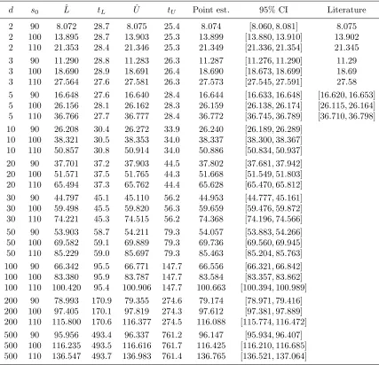
ρij =ρ for all i6=j. Our results are reported in Table 1.

Asymmetric case

As a second example, we studied model (20) with si

0 = s0, δi = δ for all i = 1,2, . . . , d, and ρij = ρ for all i 6= j, but different volatilities σ1 < σ2 < · · · < σd. For d ≤ 5, we chose the specificationσi = 0.08 + 0.32×(i−1)/(d−1), i= 1,2, . . . , d. For d >5, we set

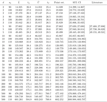
σi = 0.1 +i/(2d),i= 1,2, . . . , d. The results are given in Table 2.

4.2. Callable Multi Barrier Reverse Convertibles

A MBRC is a coupon paying security that converts into shares of the worst-performing of

d underlying assets if a prespecified trigger event occurs. Let us assume that the price of thei-th underlying asset in percent of its starting value follows the risk-neutral dynamics

Si_t= (

100 exp [r−σ2

i/2]t+σiWti

fort∈[0, Ti) 100(1−δi) exp [r−σi2/2]t+σiWti

fort∈[Ti, T]

(21)

for a risk-free interest rate r ∈ _R, volatility σi ∈ (0,∞), maturity T ∈ (0,∞), dividend payment time Ti ∈(0, T), dividend rate δi ∈[0,∞) and a d-dimensional Brownian motion

W with constant instantaneous correlationsρij ∈Rbetween different componentsWi and

Wj_.

Let us consider a MBRC that pays a coupon c at each of N time points tn = nT /N,

n= 1,2, . . . , N, and makes a time-T payment of

G= (

F if min1≤i≤dmin1≤m≤MSuim > B or min1≤i≤dS

i T > K min1≤i≤dSTi if min1≤i≤dmin1≤m≤MSuim ≤B and min1≤i≤dS

i T ≤K,

where F ∈ [0,∞) is the nominal amount, B ∈ [0,∞) a barrier, K ∈[0,∞) a strike price and um the end of the m-th trading day. Its value is

N X

n=1

e−rtn_c+e−rTE_{G (22)}

and can easily be estimated with a standard Monte Carlo approximation.

A callable MBRC can be redeemed by the issuer at any of the times t1, t2, . . . , tN−1 by paying back the notional. To minimize costs, the issuer will try to find a {t1, t2, . . . , T} -valued stopping time such that

E " _τ

X

n=1

e−rtn_{c+ 1}

{τ <T}e−rτF+ 1{τ=T}e−rTG #

is minimal.

Let (Xn)Nn=1be thed+1-dimensional Markov process given byXni =Stinfori= 1, . . . , d,

and

X_nd+1 := (

d s0 Lˆ tL Uˆ tU Point est. 95% CI Literature

2 90 8.072 28.7 8.075 25.4 8.074 [8.060,8.081] 8.075

2 100 13.895 28.7 13.903 25.3 13.899 [13.880,13.910] 13.902 2 110 21.353 28.4 21.346 25.3 21.349 [21.336,21.354] 21.345 3 90 11.290 28.8 11.283 26.3 11.287 [11.276,11.290] 11.29 3 100 18.690 28.9 18.691 26.4 18.690 [18.673,18.699] 18.69 3 110 27.564 27.6 27.581 26.3 27.573 [27.545,27.591] 27.58 5 90 16.648 27.6 16.640 28.4 16.644 [16.633,16.648] [16.620,16.653] 5 100 26.156 28.1 26.162 28.3 26.159 [26.138,26.174] [26.115,26.164] 5 110 36.766 27.7 36.777 28.4 36.772 [36.745,36.789] [36.710,36.798] 10 90 26.208 30.4 26.272 33.9 26.240 [26.189,26.289]

10 100 38.321 30.5 38.353 34.0 38.337 [38.300,38.367] 10 110 50.857 30.8 50.914 34.0 50.886 [50.834,50.937] 20 90 37.701 37.2 37.903 44.5 37.802 [37.681,37.942] 20 100 51.571 37.5 51.765 44.3 51.668 [51.549,51.803] 20 110 65.494 37.3 65.762 44.4 65.628 [65.470,65.812] 30 90 44.797 45.1 45.110 56.2 44.953 [44.777,45.161] 30 100 59.498 45.5 59.820 56.3 59.659 [59.476,59.872] 30 110 74.221 45.3 74.515 56.2 74.368 [74.196,74.566] 50 90 53.903 58.7 54.211 79.3 54.057 [53.883,54.266] 50 100 69.582 59.1 69.889 79.3 69.736 [69.560,69.945] 50 110 85.229 59.0 85.697 79.3 85.463 [85.204,85.763] 100 90 66.342 95.5 66.771 147.7 66.556 [66.321,66.842] 100 100 83.380 95.9 83.787 147.7 83.584 [83.357,83.862] 100 110 100.420 95.4 100.906 147.7 100.663 [100.394,100.989] 200 90 78.993 170.9 79.355 274.6 79.174 [78.971,79.416] 200 100 97.405 170.1 97.819 274.3 97.612 [97.381,97.889] 200 110 115.800 170.6 116.377 274.5 116.088 [115.774,116.472] 500 90 95.956 493.4 96.337 761.2 96.147 [95.934,96.407] 500 100 116.235 493.5 116.616 761.7 116.425 [116.210,116.685] 500 110 136.547 493.7 136.983 761.4 136.765 [136.521,137.064]

Table 1: Summary results for max-call options ondsymmetric assets for parameter values of r = 5%, δ = 10%, σ = 20%, ρ = 0,K = 100,T = 3, N = 9. tL is the number of seconds it took to train τΘ _{and compute ˆL. t}

U is the computation time for ˆ

d s0 Lˆ tL Uˆ tU Point est. 95% CI Literature

2 90 14.325 26.8 14.352 25.4 14.339 [14.299,14.367] 2 100 19.802 27.0 19.813 25.5 19.808 [19.772,19.829] 2 110 27.170 26.5 27.147 25.4 27.158 [27.138,27.163] 3 90 19.093 26.8 19.089 26.5 19.091 [19.065,19.104] 3 100 26.680 27.5 26.684 26.4 26.682 [26.648,26.701] 3 110 35.842 26.5 35.817 26.5 35.829 [35.806,35.835]

5 90 27.662 28.0 27.662 28.6 27.662 [27.630,27.680] [27.468,27.686] 5 100 37.976 27.5 37.995 28.6 37.985 [37.940,38.014] [37.730,38.020] 5 110 49.485 28.2 49.513 28.5 49.499 [49.445,49.533] [49.155,49.531] 10 90 85.937 31.8 86.037 34.4 85.987 [85.857,86.087]

10 100 104.692 30.9 104.791 34.2 104.741 [104.603,104.864] 10 110 123.668 31.0 123.823 34.4 123.745 [123.570,123.904] 20 90 125.916 38.4 126.275 45.6 126.095 [125.819,126.383] 20 100 149.587 38.2 149.970 45.2 149.779 [149.480,150.053] 20 110 173.262 38.4 173.809 45.3 173.536 [173.144,173.937] 30 90 154.486 46.5 154.913 57.5 154.699 [154.378,155.039] 30 100 181.275 46.4 181.898 57.5 181.586 [181.155,182.033] 30 110 208.223 46.4 208.891 57.4 208.557 [208.091,209.086] 50 90 195.918 60.7 196.724 81.1 196.321 [195.793,196.963] 50 100 227.386 60.7 228.386 81.0 227.886 [227.247,228.605] 50 110 258.813 60.7 259.830 81.1 259.321 [258.661,260.092] 100 90 263.193 98.5 264.164 151.2 263.679 [263.043,264.425] 100 100 302.090 98.2 303.441 151.2 302.765 [301.924,303.843] 100 110 340.763 97.8 342.387 151.1 341.575 [340.580,342.781] 200 90 344.575 175.4 345.717 281.0 345.146 [344.397,346.134] 200 100 392.193 175.1 393.723 280.7 392.958 [391.996,394.052] 200 110 440.037 175.1 441.594 280.8 440.815 [439.819,441.990] 500 90 476.293 504.5 477.911 760.7 477.102 [476.069,478.481] 500 100 538.748 504.6 540.407 761.6 539.577 [538.499,540.817] 500 110 601.261 504.9 603.243 760.8 602.252 [600.988,603.707]

Table 2: Summary results for max-call options ondasymmetric assets for parameter values of r= 5%, δ = 10%, ρ= 0, K = 100,T = 3, N = 9. tL is the number of seconds it took to trainτΘ _{and compute ˆL. t}

Then the issuer’s minimization problem can be written as

inf

τ∈T Eg(τ, Xτ), (23)

whereT is the set of allX-stopping times and

g(n, x) = (_Pn

m=1e

−rtm_c+e−rtn_{F if 1≤n≤N−1 orx}d+1 _{= 0}

PN m=1e

−rtm_c+e−rtN_{h(x) ifn=N and x}d+1_{= 1,}

where

h(x) = (

F if min1≤i≤dxi > K min1≤i≤dxi if min1≤i≤dxi ≤K.

Since the issuer cannot redeem at time 0, we trained stopping times of the form

τΘ₌ N X

n=1

nfθn_(Y

n) n−1

Y

j=1

(1−fθj_(Y

k))∈ T1

forfθN _{≡1 andf}θ1_{, . . . , f}θN−1_:Rd+1_{→ {0,1}given by (8) withI = 2 andq}

1 =q2 =d+40. Since (23) is a minimization problem, τΘ _{yields an upper bound and the dual method a} lower bound.

We simulated the model (21) like (20) in Subsection 4.1 with the same number of trials except that here we used the lower numberJ = 1,024 to estimate the dual bound. Numerical results are reported in Table 3.

4.3. Optimally Stopping a Fractional Brownian Motion

A fractional Brownian motion with Hurst parameter H ∈ (0,1] is a continuous centered Gaussian process (WH

t )t≥0 with covariance structure E[W_tHW_sH] = 1

2 t

2H _+s2H _{− |t−s|}2H ;

see, e.g., Mandelbrot and Van Ness (1968) or Samoradnitsky and Taqqu (1994). For H = 1/2, WH _{is a standard Brownian motion. So, by the optional stopping theorem, one} has EWτ1/2 = 0 for every W1/2-stopping time τ bounded above by a constant; see, e.g., Grimmett and Stirzaker (2001). However, forH6= 1/2, the increments ofWH _{are correlated} – positively forH ∈(1/2,1] and negatively forH∈(0,1/2). In both cases,WH _{is neither a} martingale nor a Markov process, and there exist boundedWH_{-stopping timesτ such that} EWH

τ > 0; see, e.g., Kulikov and Gusyatnikov (2016) for two classes of simple stopping rules 0≤τ ≤1 and estimates of the corresponding expected valuesEWH

τ . To approximate the supremum

sup 0≤τ≤1E

d ρ Lˆ tL Uˆ tU Point est. 95% CI Non-callable

2 0.6 98.235 24.9 98.252 204.1 98.243 [98.213,98.263] 106.285 2 0.1 97.634 24.9 97.634 198.8 97.634 [97.609,97.646] 106.112 3 0.6 96.930 26.0 96.936 212.9 96.933 [96.906,96.948] 105.994 3 0.1 95.244 26.2 95.244 211.4 95.244 [95.216,95.258] 105.553 5 0.6 94.865 41.0 94.880 239.2 94.872 [94.837,94.894] 105.530 5 0.1 90.807 41.1 90.812 238.4 90.810 [90.775,90.828] 104.496 10 0.6 91.568 71.3 91.629 300.9 91.599 [91.536,91.645] 104.772 10 0.1 83.110 71.7 83.137 301.8 83.123 [83.078,83.153] 102.495 15 0.6 89.558 94.9 89.653 359.8 89.606 [89.521,89.670] 104.279 15 0.1 78.495 94.7 78.557 360.5 78.526 [78.459,78.571] 101.209 30 0.6 86.089 158.5 86.163 534.1 86.126 [86.041,86.180] 103.385 30 0.1 72.037 159.3 72.749 535.6 72.393 [71.830,72.760] 99.279

Table 3: Summary results for callable MBRCs with dunderlying assets for F =K = 100,

B = 70, T = 1 year (= 252 trading days), N = 12, c= 7/12,δi = 5%, Ti = 1/2,

r = 0, σi = 0.2 and ρij = ρ for i 6= j. tU is the number of seconds it took to trainτΘ _{and compute ˆU. t}

L is the number of seconds it took to compute ˆL. The last column lists fair values of the same MBRCs without the callable feature. We estimated them by averaging 4,096,000 Monte Carlo samples of the payoff. This took between 5 (ford= 2) and 44 (for d= 30) seconds.

over all WH_{-stopping times 0 ≤ τ ≤ 1, we denote t}

n = n/100, n = 0,1,2, . . . ,100, and introduce the 100-dimensional Markov process (Xn)100n=0 given by

X0 = (0,0, . . . ,0)

X1 = (WtH1,0, . . . ,0)

X2 = (WtH2, W H

t1,0, . . . ,0) ..

.

X100 = (Wt100H , Wt99H, . . . , Wt1H). The discretized stopping problem

sup τ∈T E

g(Xτ), (25)

whereT is the set of allX-stopping times andg:R100_{→Rthe projection (x}1_{, . . . , x}100_)7→

x1_{, approximates (24) from below.}

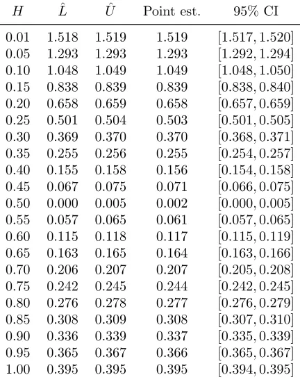
We computed estimates of (25) forH∈ {0.01,0.05,0.1,0.15, . . . ,1}by training networks of the form (8) with depth I = 2, d= 100 and q1 =q2 = 140. To simulate the vector Y = (WH

tn)

100

k = 1, . . . , KU of Z and set wk = Bvk. Then we produced another KU ×J simulations ˜

vk,j_{,k = 1, . . . , K}

U, j = 1, . . . , J, of Z, and generated for all nand k, continuation paths starting from

z_nk= (w_nk, . . . , wk₁,0, . . . ,0) according to

˜

z_mk,j = ( ˜w_mk,j, . . . ,w˜k,j_n+1, w_nk, . . . , wk₁,0. . . ,0), m=n+ 1, . . . ,100,

with

˜

w_lk,j= n X

i=1

Blivik+ l X

i=n+1

Bliv˜k,ji , l=n+ 1, . . . , m.

For H ∈ {0.01, ...,0.4} ∪ {0.6, ...,1.0}, we chose J = 16,384, and forH ∈ {0.45,0.5,0.55},

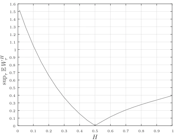
J = 32,768. The results are listed in Table 4 and depicted in graphical form in Figure 1. Note that for H = 1/2 and H = 1, our 95% confidence intervals contain the true values, which in these two cases, can be calculated exactly. As mentioned above,W1/2_{is a Brownian} motion, and therefore,EWτ1/2= 0 for every (Wt1/2n )

100

n=0-stopping timeτ. On the other hand, one has18 _W1

t =tW11,t≥0. So, in this case, the optimal stopping time is given18 by

τ = (

1 ifW1 t1 >0

t1 ifWt11 ≤0, and the corresponding expectation by

EW_τ1=E

W₁11n

W_t1 1>0

o−W1

t11n

W_t1 1≤0

o

= 0.99EhW₁11_{W1 1>0}

i

= 0.99/√2π= 0.39495...

Moreover, it can be seen that for H ∈(1/2,1), our estimates are up to three times higher than the expected payoffs generated by the heuristic stopping rules of Kulikov and Gusy-atnikov (2016). For H∈(0,1/2), they are up to five times higher.

Acknowledgments

We thank Philippe Ehlers, Ariel Neufeld, Martin Stefanik, the action editor and the referees for fruitful discussions and helpful comments.

References

Charalambos D. Aliprantis and Kim C. Border. Infinite Dimensional Analysis. Springer, Berlin, 3rd Edition, 2006.

Leif Andersen. A simple approach to the pricing of Bermudan swaptions in the multifactor LIBOR market model. The Journal of Computational Finance, 3(2):5–32, 2000.

H Lˆ Uˆ Point est. 95% CI

0.01 1.518 1.519 1.519 [1.517,1.520] 0.05 1.293 1.293 1.293 [1.292,1.294] 0.10 1.048 1.049 1.049 [1.048,1.050] 0.15 0.838 0.839 0.839 [0.838,0.840] 0.20 0.658 0.659 0.658 [0.657,0.659] 0.25 0.501 0.504 0.503 [0.501,0.505] 0.30 0.369 0.370 0.370 [0.368,0.371] 0.35 0.255 0.256 0.255 [0.254,0.257] 0.40 0.155 0.158 0.156 [0.154,0.158] 0.45 0.067 0.075 0.071 [0.066,0.075] 0.50 0.000 0.005 0.002 [0.000,0.005] 0.55 0.057 0.065 0.061 [0.057,0.065] 0.60 0.115 0.118 0.117 [0.115,0.119] 0.65 0.163 0.165 0.164 [0.163,0.166] 0.70 0.206 0.207 0.207 [0.205,0.208] 0.75 0.242 0.245 0.244 [0.242,0.245] 0.80 0.276 0.278 0.277 [0.276,0.279] 0.85 0.308 0.309 0.308 [0.307,0.310] 0.90 0.336 0.339 0.337 [0.335,0.339] 0.95 0.365 0.367 0.366 [0.365,0.367] 1.00 0.395 0.395 0.395 [0.394,0.395]

H

su

pτ

E

W

H τ

0 0 0.1

0.1 0.2

0.2 0.3

0.3 0.4

0.4 0.5

0.5 0.6

0.6 0.7

0.7 0.8

0.8 0.9

0.9 1

1 1.1

1.2 1.3 1.4 1.5 1.6

Figure 1: Estimates of sup_τ∈{0,t1,...,1}EWτH for different values ofH.

Leif Andersen and Mark Broadie. Primal-dual simulation algorithm for pricing multidimen-sional American options. Management Science, 50(9):1222–1234, 2004.

Vlad Bally, Gilles Pag`es, and Jacques Printems. A quantization tree method for pricing and hedging multidimensional American options. Mathematical Finance, 15(1):119–168, 2005.

J´erˆome Barraquand and Didier Martineau. Numerical valuation of high dimensional mul-tivariate American securities. The Journal of Financial and Quantitative Analysis, 30(3):383–405, 1995.

Denis Belomestny. On the rates of convergence of simulation-based optimization algorithms for optimal stopping problems. The Annals of Applied Probability, 21(1):215–239, 2011.

Denis Belomestny. Solving optimal stopping problems via empirical dual optimization. The Annals of Applied Probability, 23(5):1988–2019, 2013.

Denis Belomestny, Christian Bender, and John Schoenmakers. True upper bounds for Bermudan products via non-nested Monte Carlo. Mathematical Finance, 19(1):53–71, 2009.

Denis Belomestny, Mark Joshi, and John Schoenmakers. Multilevel dual approach for pricing American style derivatives. Finance and Stochastics, 17(4):717–742, 2013.

Steffan J. Berridge and Johannes M. Schumacher. An irregular grid approach for pricing high-dimensional American options. Journal of Computational and Applied Mathematics, 222(1):94–111, 2008.

Phelim P. Boyle, Adam W. Kolkiewicz, and Ken Seng Tan. An improved simulation method for pricing high-dimensional American derivatives. Mathematics and Computers in Sim-ulation, 62:315–322, 2003.

Mark Broadie and Menghui Cao. Improved lower and upper bound algorithms for pricing American options by simulation. Quantitative Finance, 8(8):845–861, 2008.

Mark Broadie and Paul Glasserman. A stochastic mesh method for pricing high-dimensional American options. The Journal of Computational Finance, 7(4):35–72, 2004.

Jacques F. Carriere. Valuation of the early-exercise price for options using simulations and nonparametric regression. Insurance: Mathematics and Economics, 19(1):19–30, 1996.

Nan Chen and Paul Glasserman. Additive and multiplicative duals for American option pricing. Finance and Stochastics, 11(2):153–179, 2007.

Mark H. A. Davis and Ioannis Karatzas. A deterministic approach to optimal stopping. In

Probability, Statistics and Optimisation: A Tribute to Peter Whittle (ed. Frank P. Kelly), pages 455–466. John Wiley & Sons, NewYork, 1994.

Vijay V. Desai, Vivek F. Farias, and Ciamac C. Moallemi. Pathwise optimization for optimal stopping problems. Management Science, 58(12):2292–2308, 2012.

Daniel Egloff, Michael Kohler, and Nebojsa Todorovic. A dynamic look-ahead Monte Carlo algorithm for pricing Bermudan options. The Annals of Applied Probability, 17(4):1138– 1171, 2007.

Diego Garc´ıa. Convergence and biases of Monte Carlo estimates of American option prices using a parametric exercise rule. Journal of Economic Dynamics and Control, 27(10):1855–1879, 2003.

Xavier Glorot and Yoshua Bengio. Understanding the difficulty of training deep feedforward neural networks. In Proceedings of the Thirteenth International Conference on Artificial Intelligence and Statistics,PMLR, 9:249–256, 2010.

Geoffrey Grimmett and David Stirzaker. Probability and Random Processes. Oxford Uni-versity Press, 3rd Edition, 2001.

Jiequn Han and Weinan E. Deep learning approximation for stochastic control problems.

Deep Reinforcement Learning Workshop, NIPS, 2016.

Martin B. Haugh and Leonid Kogan. Pricing American options: a duality approach. Oper-ations Research, 52(2):258–270, 2004.

Shashi Jain and Cornelis W. Oosterlee. The stochastic grid bundling method: efficient pricing of Bermudan options and their Greeks. Applied Mathematics and Computation, 269:412–431, 2015.

Farshid Jamshidian. The duality of optimal exercise and domineering claims: a Doob–Meyer decomposition approach to the Snell envelope. Stochastics, 79:27–60, 2007.

Diederik P. Kingma and Jimmy Ba. Adam: A method for stochastic optimization. Inter-national Conference on Learning Representations, 2015.

Michael Kohler, Adam Krzy˙zak, and Nebojsa Todorovic. Pricing of high-dimensional Amer-ican options by neural networks. Mathematical Finance, 20(3):383–410, 2010.

Anastasia Kolodko and John Schoenmakers. Iterative construction of the optimal Bermudan stopping time. Finance and Stochastics, 10(1):27–49, 2006.

Alexander V. Kulikov and Pavel P. Gusyatnikov. Stopping times for fractional Brown-ian motion. In Computational Management Science, Volume 682 of Lecture Notes in Economics and Mathematical Systems, pages 195–200. Springer International Publishing, 2016.

Damien Lamberton and Bernard Lapeyre. Introduction to Stochastic Calculus Applied to Finance. Chapman & Hall/CRC, 2nd Edition, 2008.

J´erˆome Lelong. Pricing American options using martingale bases. arXiv:1604.03317, 2016.

Moshe Leshno, Vladimir Ya. Lin, Allan Pinkus, and Shimon Schocken. Multilayer feedfor-ward networks with a nonpolynomial activation function can approximate any function.

Neural Networks, 6(6):861–867, 1993.

Timothy P. Lillicrap, Jonathan J. Hunt, Alexander Pritzel, Nicolas Heess, Tom Erez, Yuval Tassa, David Silver, and Daan Wierstra. Continuous control with deep reinforcement learning. International Conference on Learning Representations, 2016.

Francis A. Longstaff and Eduardo S. Schwartz. Valuing American options by simulation: a simple least-squares approach. The Review of Financial Studies, 14(1):113–147, 2001.

Benoit B. Mandelbrot and John W. Van Ness. Fractional Brownian motions, fractional noises and applications. SIAM Review, 10(4):422–437, 1968.

Volodymyr Mnih, Koray Kavukcuoglu, David Silver, Andrei A. Rusu et al. Human-level control through deep reinforcement learning. Nature, 518:529–533, 2015.

Goran Peskir and Albert N. Shiryaev. Optimal Stopping and Free-Boundary Problems. Lectures in Mathematics. Birkh¨auser Basel, 2006.

Chris Rogers. Monte Carlo valuation of American options. Mathematical Finance, 12(3):271–286, 2002.

Gennady Samoradnitsky and Murad S. Taqqu. Stable Non-Gaussian Random Processes. Chapman and Hall/CRC, 1994.

John Schulman, Sergey Levine, Philipp Moritz, Michael Jordan, and Pieter Abbeel. Trust region policy optimization. In Proceedings of the 32nd International Conference on Ma-chine Learning,PMLR, 37:1889–1897, 2015.

Martin Schweizer. On Bermudan options. In Advances in Finance and Stochastics, pages 257–270. Springer Berlin Heidelberg, 2002.

David Silver, Aja Huang, Chris J. Maddison, Arthur Guez et al. Mastering the game of Go with deep neural networks and tree search. Nature, 529:484–489, 2016.

Justin Sirignano and Konstantinos Spiliopoulos. DGM: A deep learning algorithm for solv-ing partial differential equations.Journal of Computational Physics, 375:1339–1364, 2018.

Richard S. Sutton and Andrew G. Barto. Reinforcement Learning. The MIT Press, 1998.

James A. Tilley. Valuing American options in a path simulation model. Transactions of the Society of Actuaries, 45:83–104, 1993.