The Thirty-Third AAAI Conference on Artificial Intelligence (AAAI-19)
Understanding Learned Models by
Identifying Important Features at the Right Resolution
Kyubin Lee
*Clinical Genomics Analysis Branch National Cancer Center
Republic of Korea
Akshay Sood
* Dept. of Computer Sciences Dept. of Biostatistics & Medical InformaticsUniversity of Wisconsin-Madison
*These authors contributed equally to this work.
Mark Craven
Dept. of Biostatistics & Medical Informatics Dept. of Computer Sciences University of Wisconsin-Madison
Abstract
In many application domains, it is important to characterize how complex learned models make their decisions across the distribution of instances. One way to do this is to identify the features and interactions among them that contribute to a model’s predictive accuracy. We present a model-agnostic approach to this task that makes the following specific contri-butions. Our approach (i) tests feature groups, in addition to base features, and tries to determine the level of resolution at which important features can be determined, (ii) uses hypoth-esis testing to rigorously assess the effect of each feature on the model’s loss, (iii) employs a hierarchical approach to con-trol the false discovery rate when testing feature groups and individual base features for importance, and (iv) uses hypothe-sis testing to identify important interactions among features and feature groups. We evaluate our approach by analyzing random forest and LSTM neural network models learned in two challenging biomedical applications.
Introduction
In many application domains, it is important to be able to inspect, probe, and understand models learned by machine-learning systems. There are several principal reasons why it might be critical to understand how learned models make their decisions: (i)Trust: end users and other stakeholders need to trust the models’ decisions and understand the basis for them in order for the models to be accepted and employed; (ii)Model development: to help improve the predictive per-formance of models, interpretable descriptions can aid in selecting among models, detecting and avoiding overfitting, and gaining insight into differences among input representa-tions; (iii)Discovery: our knowledge of a problem domain can be augmented by identifying previously unrecognized salient features and relationships that models have learned.
In such application domains, there is a strong incentive to use a learning method that directly learns interpretable mod-els, such as logistic regression or a generalized additive model (Lou et al. 2013). However, there is often tension between the desiderata of model comprehensibility and predictive performance. It may be the case that the machine-learning approaches that provide the best predictive performance in a
Copyright c2019, Association for the Advancement of Artificial Intelligence (www.aaai.org). All rights reserved.
given domain learn models that are highly challenging to in-spect and understand. For this reason, a number of approaches have been developed for gaining insight into complex learned models such as random forests and deep neural networks.
Methods for gaining comprehensible descriptions of learned models can be divided into two broad categories. The first category, which is referred to as prediction in-terpretability encompasses methods that lend insight into learned models by locally explaining the decisions they make for individual instances (Alvarez-Melis and Jaakkola 2017; Fong and Vedaldi 2017; Koh and Liang 2017; Lei, Barzi-lay, and Jaakkola 2016; Leino et al. 2018; Ribeiro, Singh, and Guestrin 2016; 2018). The second category, referred to asmodel interpretability, refers to methods that aim to provide characterizations of how models make decisions across the distribution of instances. Some methods in this category are tailored to specific types of models (Bau et al. 2017; Bojarski et al. 2017; Hara and Hayashi 2018; Karpathy, Johnson, and Fei-Fei 2016), whereas others are agnostic to the model type (Craven and Shavlik 1996; Ribeiro, Singh, and Guestrin 2016; 2018).
when testing feature groups and base features for importance. Third, we propose a method based on hypothesis testing to identify important interactions among base features and feature groups.
We evaluate our approach by analyzing random forest and LSTM neural network models learned in two application domains: identifying viral genotype-to-disease-phenotype associations, and predicting asthma exacerbations from elec-tronic health records (EHRs). Additionally, we validate our approach using synthetic data sets in which we know which features and groups are truly important.
Methods
In this section, we describe the key elements of the model-agnostic approach we have developed for characterizing learned models. The source code for our methods is available at https://github.com/Craven-Biostat-Lab/mihifepe.
Identifying Important Features via Perturbation
As shown in Algorithm 1, a general approach to identifying important features in a learned model is to measure how the output of the model, or its loss, varies when individual features in a given set of instances are perturbed in some way. Breiman (2001) proposed an approach based on this idea as a way to characterize learned random forest models, and Friedman proposed a similar approach for generatingpartial dependency plots(Friedman 2001; Friedman and Popescu 2008). In Breiman’s method, the perturbation is done by permuting the values of the given feature across a set of instances. However, the approach can be generalized to other perturbations, including feature “erasure” (Li, Monroe, and Jurafsky 2016), flipping binary features, or replacing features with “background” values.
Algorithm 1:General approach to identifying important
features via perturbation
input :learned modelh, feature setF, test set
T ={ x(1), y(1)
. . . x(m), y(m)
}
output :set{(j, vj)|j∈F}summarizing the effectvj
on lossLwhen perturbing each featurej
foreachfeaturej ∈Fdo
foreachinstance x(i), y(i)inTdo
let∆x(ji)representx(i)with featurejperturbed
in some way compare lossL
y(i), h x(i)
to
Lhy(i), h∆x(i)
j i
calculate summary statisticvjcharacterizing the
effect of perturbing featurejonL
A key extension of this idea in our approach is that it uses hypothesis testing to determine whether a given feature has a generally consistent effect on the model’s loss across the distribution of instances. We do this using held-aside
test instances so that our importance assessment measures whether a feature truly impacts a model’s predictive accuracy. In the results presented here, we use the Wilcoxon matched-pairs signed-rank test to assess the null hypothesis that the median difference between pairs:
Lhy(i), hx(i) i− 1
P
P X
p=1
Lhy(i), h∆x(ji,p) i (1)
is zero. Here ∆x(ji,p)is defined asx(i)with featurej per-turbed on thepthpermutation. For perturbations that do not involve randomness, such as erasure,P = 1andx(ji,1) de-notes the single perturbation that can be done to featurej.
We use the Wilcoxon test in place of a pairedt-test due to significant non-normality in the changes to loss introduced by feature perturbations. Here, we use the one-tailed version of the test, corresponding to the median difference beinggreater than zero, in order to focus on features that provide predictive value to the model. Alternatively, we could use a two-tailed test to also detect features whose perturbationdecreasesloss, thereby indicating overfitting.
Considering Feature Groups
The approach described in Algorithm 1 is typically applied to the set of features that are used as input to the model, which we refer to asbase features. We argue that, in many domains, characterizing the importance of base features may not be the right level of resolution for gaining a thorough understanding of a learned model. In some domains, there may be a large number of features that are important to the model, and it may be difficult to discern which high-level factors are most important for the model’s predictions unless groupings of related features are considered. For example models that perform risk assessment from electronic health records often have thousands of base features representing distinct diagnoses. Our understanding of such a model is likely to be aided by analyzing the importance of groups of related diagnoses, or even the entire set of diagnoses, in addition to very specific ones. Moreover, it might be the case that few, if any, individual base features show a statistically significant change to the model’s loss when perturbed, or the effect sizes of these changes to the loss are small. In such cases, we can potentially detect statistical significance and larger effect sizes by considering groups of related features. In contrast to assessing feature importance only at the level of base features, our approach also assesses the importance offeature groups. We assume that we are given a hierarchy in which internal nodes represent groups of features, and leaf nodes represent base features. We can then apply Algorithm 1 to both base features and feature groups in order to determine which are important.
the occurrence of specific recorded diagnoses in a given pa-tient’s EHR, such asreflux esophagitis(ICD-9 code 530.11) oracute esophagitis(ICD-9 530.12). We could test the im-portance of such features by erasing all occurrences of the given diagnosis from patients’ records and measuring the resulting loss. Moreover, we might test the importance of the feature groupsesophagitis(ICD-9 530.1), which has five children diagnoses including the two listed above, or
diseases of the esophagus(ICD-9 530), which has 28 descendant diagnoses. To test a feature group, we could erase all recorded diagnosis that are encompassed by the group.
In other application domains, the feature groups might be derived from data. For example, in our viral genotype-to-phenotype task, we calculate feature groups using a hierar-chical clustering method. Our base features arehaplotype blocks, which are variable-sized regions of the genome that have been inherited as a unit from one of two parental virus strains. Our feature groups consist of sets of neighboring haplotype blocks (i.e., larger regions of the viral genome).
In a natural language domain, we might define feature groups on the basis of syntactic or semantic categories. In an image classification domain, the base features might cor-respond to pixels and we might define feature groups to represent superpixels or objects as feature groups. Perturba-tions could involve replacing a region with a constant value, injecting noise, or blurring (Fong and Vedaldi 2017).
In domains with temporal or sequential input, feature groups could represent sets of features with restrictions based on their occurrence in time/sequence. For example, in a clini-cal risk-assessment domain we might define feature groups representing occurrences of diagnoses restricted to certain time windows, such asdiseases of the esophaguswithin the past year, oresophagitiswhen patient’s age>50.
In contrast to approaches for hierarchical feature selec-tion (Wan and Freitas 2018), the hierarchies used by our approach do not necessarily representis-aor generalization-specializationrelationships. Each internal node needs only to group features that are related in some meaningful way (e.g., neighboring regions of a genome). Moreover, our ap-proach is not focused on feature selection per se, but instead on characterizing which feature groups are important in a given learned model.
Controlling the False Discovery Rate
Given a hierarchy over the features, we can compute the effect of perturbing each base feature and each feature group using Algorithm 1 across a given set of instances. We treat each node in the hierarchy as representing the null hypothesis that perturbing the corresponding feature group does not have a significant effect on the loss function, in the sense that the median of the differences computed using Formula (1) is zero. A hypothesis is rejected if this median difference is statistically significantly different from zero, and a hypothesis is tested only if its parent hypothesis has been rejected.
However, there is a notable multiple-comparisons problem due to the potentially large number of hypotheses tested. For instance, there are 8,740 hypotheses to be tested (counting both base features and feature groups) in the asthma exac-erbation prediction task that we address. Moreover, when
adjusting for multiple comparisons, we need to take into account the hierarchical organization of the hypotheses be-ing tested. We address this issue by usbe-ing the hierarchical false discovery rate (FDR) control methodology developed by Yekutieli (2008) as described in Algorithm 2.
This algorithm uses a recursive procedure to consider a hierarchical set of hypotheses, which in our case consist of feature groups to be tested. If the null hypothesis is rejected for a given node in the hierarchy (i.e., we determine that a feature group is important), then the children of that node are tested using the Benjamini-Hochberg method (Benjamini and Hochberg 1995) to control false discoveries. Otherwise, the descendants of the given node are not tested. The algorithm returns a subtree representing the set of feature groups and base features for which the null hypothesis was rejected.
Using this algorithm, we can identify the set of feature groups and base features that have a significant effect on a model’s loss while controlling the rate of false discoveries in this set. Of particular interest is the set ofouternodes: those nodes for which we reject the null hypotheses (i.e., determine that they are important) that have no children for which we reject the null hypotheses. These nodes represent the finest level of resolution at which we can determine the importance of features and feature groups.
The key assumptions made by this approach, which are reasonable in our context, are that (i) if a given feature signif-icantly affects the loss when perturbed, a group of features containing this feature will also significantly affect the loss when perturbed, (ii) thep-values for siblings are indepen-dently distributed, and (iii)p-values for true null hypotheses are uniformly distributed in [0,1].
Identifying Important Interactions
In addition to identifying individual base features and feature groups that are important, we would also like to identify in-teractions among them that a given model has determined as important. Here we consider cases in which the model outputs a scalar value. For this analysis, we do not treat a given model completely as a black box, but instead as-sume that we know the transfer function that produces the model’s outputs. Letg(x(i))denote the function that maps
x(i)to the value that is input to the transfer functionf(·), andh x(i)
=f g(x(i))
indicate the output of the model. For example,f(·)might be a logistic activation function in a neural network for a binary classification task, in which case
g(·)would represent the part of the network that maps from x(i)to the net input of the logistic function. Or in a random
forest trained for a regression task,f(·)would represent the identity function, andg(·)would represent the average of the values predicted by the individual trees in the forest.
Our notion of an interaction among features is based on the concept of additivity. We define an interaction between featurejand featurekto mean that changes ing(·)when we perturb both features are non-additive (for some instances):
h
g∆x(ji)−gx(i)i+hg∆x(ki)−gx(i)i6≈
h
Algorithm 2:Using hierarchical FDR control to identify important features
input :TreeTof hypotheses to be tested along with
their associatedp-values, significance levelq
output :A subtreeSofTcorresponding to hypotheses
rejected while controlling FDR at significance levelq
function HierarchicalFDR(node):
// node has already been rejected rejectedSet={node}
if nodeis not leafthen
letP(1)≤. . .≤P(k)be the set of ordered
p-values ofnode.children
// Apply Benjamini-Hochberg procedure to children
letr= max{i:P(i)≤i×kq}
ifr >0then
rejectedChildren=set ofrhypotheses corresponding toP(1)≤. . .≤P(r)
foreach child∈rejectedChildrendo
rejectedSet=rejectedSet∪ HierarchicalFDR(child)
returnrejectedSet
begin
if T.root.pvalue> qthen
S= empty tree
else
S=HierarchicalFDR(T.root)
where∆x(ji∧)kdenotes instancex(i)with featurejand feature
kjointly perturbed.
To identify interactions that are important, we use hypoth-esis testing to assess whether a candidate interaction exhibits nonadditivity. We can do this by considering the median difference between pairs formed by the two sides of the inequality above. In the results presented here, we use the Wilcoxon matched-pairs signed-rank test to assess the null hypothesis that the median difference between the pairs is zero. This approach to testing interactions can be applied to base features, feature groups, and mixtures thereof.
Alternatively, we can consider whether a candidate interac-tion exhibits nonadditivity which has a generally consistent effect on the model’s loss across the distribution of instances. We can do this by assessing the difference between pairs:
Lhy(i), fg ∆x(ji∧)ki
−
Lhy(i), fg x(i)
+ ∆g ∆x(ji)
+ ∆g ∆x(ki)i
(3)
where∆g ∆x(ji)
is defined ashg ∆x(ji)
−g x(i)i
(i.e.,
the change ing(x(i))that results from perturbing featurej).
However, the null distribution may not be as straightforward to work with in this case because, depending on the loss function, the difference in variances of the inner terms on each side may lead to the loss terms having different means. A related approach that can be used to detect interactions is theH2 statistic (Friedman and Popescu 2008) which is
based on partial dependency scores.
Results
In this section, we evaluate our approach by (i) assessing its ability to detect important features and interactions while controlling FDR on synthetic data sets, and (ii) applying it in two biomedical domains in which it is essential to understand learned models.
Evaluation on Synthetic Data Sets
To verify that our approach is able to identify important features and interactions while controlling the false discovery rate, we first evaluate it using data sets for which we know the truly important features. In this setting we can think of each model as approximating a ground-truth function of the form:
y(i)= X
j∈IL
αjx
(i)
j +
X
(j,k)∈II
j6=k
αjkx
(i)
j x
(i)
k (4)
where IL andII represent the subset of important linear
and interaction terms respectively, andαjandαjkare
corre-sponding coefficients that determine how thejthfeature and (j, k)thinteraction contribute to the output. Note that a feature is considered important if belongs toIL, or is a component
of an interaction that belongs toII, or both. We represent a
“learned” model using the following form:
hx(i)= X
j∈IL
αjx
(i)
j +
X
(j,k)∈II
j6=k
αjkx
(i)
j x
(i)
k +γ
(i) (5)
where γ(i) ∼ N(0, σ2) represents the deviation of the model’s output from the ground-truth function for some in-stanceiin the feature space. This formulation is intended to simulate the situation in which a learned model provides a fairly accurate representation of the underlying target func-tion, but incorporates irrelevant features and other deviations which have a small impact on the model’s outputs.
We generate synthetic data sets by drawing feature vec-tors from a given distribution, and then using Equation 5 to determineh(x(i))for eachx(i), and similarly for each perturbation ofx(i). Here we present results in which our
in-stance spaces have 500 binary features, and each underlying ground truth function has 50 important features and 50 impor-tant interactions selected from among these, with coefficients
αj ∼U(0,1) ∀j ∈ILandαjk ∼ U(0,1) ∀(j, k) ∈II.
subtree. We use Equation 1 for hypothesis testing of the fea-tures, performing perturbations by erasure (i.e., setting the feature to zero in all instances), followed by the hierarchical FDR procedure (Algorithm 2) withq= 0.05.
To analyze interactions, we use the (base) features identi-fied as important in the preceding analysis to construct a set of potential interactions to test. This allows us to prune the large search space of all possible interactions, albeit at the cost of decreased power. We then use Equation 2 to perform hy-pothesis testing of these interactions, and use the Benjamini-Hochberg procedure (1995) to control FDR among this set.
features interactions
m FDR power FDR power
32 0.019 0.722 0.046 0.132
64 0.024 0.800 0.014 0.370
128 0.026 0.850 0.030 0.543
256 0.029 0.895 0.035 0.682
512 0.036 0.919 0.040 0.777
1024 0.035 0.936 0.039 0.840
2048 0.029 0.948 0.048 0.877
4096 0.029 0.960 0.045 0.913
8192 0.033 0.967 0.046 0.935
16384 0.032 0.975 0.039 0.949
(a)
features interactions
σ FDR power FDR power
0.00 0.000 0.999 0.000 0.991
0.01 0.034 0.983 0.048 0.966
0.02 0.034 0.982 0.047 0.964
0.04 0.034 0.980 0.048 0.958
0.08 0.034 0.974 0.048 0.945
0.16 0.034 0.964 0.049 0.920
0.32 0.034 0.938 0.048 0.866
0.64 0.033 0.887 0.049 0.766
1.28 0.033 0.770 0.050 0.564
(b)
Table 1: FDR and power on synthetic data sets as (a) the size of the test setmis varied (b)σis varied.
Table 1a shows the results of applying our method as the number of instances in the “test set” is varied. The results in the table represent averages over 100 randomly generated models and datasets. For each test-set size, we report both the mean power of the method (i.e., the fraction of the truly important features and interactions that are identified as such) and the mean false discovery rate (i.e., the fraction of puta-tively important features and interactions that are not truly important). The middle columns show FDR and power when determining important features and feature groups, and the rightmost columns show FDR and power when determining important interactions. Table 1b shows the effect of varying
σ when sampling theγ(i) values for each learned model.
Here, the number of instances is 10,000. The results in Ta-bles 1a and 1b indicate, not surprisingly, that the power of our method to detect truly important features and interactions
increases with larger test sets, and decreases with larger val-ues ofσ. Importantly, for all conditions, the FDR≤0.05as expected with our approach.
The analyses of both features and interactions show similar trends. However, the mean power for discovering important interactions trails the mean power for discovering important features for any given test set size/noise level. This is because we only test an interaction if its constituent features have already been found to be important during the preceding feature analysis.
Real Application Domains and Models
The first real domain we consider is focused on identify-ing the genetic components of Herpes simplex virus type 1 (HSV-1) that are responsible for various dimensions of eye disease. Here we analyze random-forest models that have learned mappings from variations in viral genotypes to three different eye disease phenotypes (Kolb et al. 2016; Lee et al. 2016). Each instance corresponds to a genetically distinct strain of the virus, and there are 65 recombinant strains generated by mixed infection of two parental strains. We represent each genotype as a vector of 547 features, where each feature corresponds to ahaplotype blockwhich is variable-sized regions of the genome that has been inher-ited as a unit from one of the two parental virus strains. The value of each binary feature indicates from which parental strain the haplotype block was inherited. The phenotypes (ble-pharitis, stromal keratitis, and neovascularization) for each instance are numeric scores indicating the disease severity re-sulting from infection in mice by a given strain. The random-forest (RF) regression models had statistically significant predictability for all three phenotypes and they demonstrated better cross-validated predictive accuracy than penalized lin-ear regression models (Lasso and Ridge) for two of these three phenotypes, and others we have assessed. The cross-validatedR2values for the blepharitis, stromal keratitis, and
neovascularization models are 0.45, 0.56, and 0.48, respec-tively. Each learned RF model comprises 1,000 trees.
The second application domain we address is to predict asthma exacerbations from electronic health records. The data set consists of information derived from EHRs for a cohort of 28,101 asthma patients from the University of Wis-consin Health System over a five-year period. The infor-mation extracted from the EHRs includes demographic fea-tures and time-stamped events corresponding to encounters with the healthcare system. These events include problem-list and other coded diagnoses, procedures, medications, vi-tals, asthma control scores, and prior exacerbations. We also include features representing the time since the last event, represented at multiple scales.
problem diagnoses, and interventions (procedures and med-ications) all comprise large vocabularies (6,533 for coded diagnoses, 4,398 for problem diagnoses, and 8,745 for inter-ventions) of which only a small subset is recorded at each encounter. Therefore, we first map event vectors for each of these sets to an embedded space using Med2Vec (Choi et al. 2016), resulting in shorter, dense fixed-length vectors. Separate embeddings of size 200 were generated for each of these sets, which were then concatenated, along with the other temporal features, to produce the event representation at each timestamp in the record. The ordered sequence of events formed the input sequence for the LSTM. The static demographic features were provided as input at the output sigmoid layer. Using 10-fold cross-validation to assess the predictive accuracy of the networks results in an area under the ROC curve (AUROC) of 0.757.
Feature Groups and Perturbations
For the HSV-1 application, our feature hierarchy represents neighboring regions of the viral genome. We compute the hierarchy using a constrained hierarchical clustering method applied to the base features, which represent haplotype blocks. This clustering method uses Hamming distance to compare columns (features) in our data matrix, and a complete linkage function, such that every pair of features in a given cluster is within a specified bit difference. The agglomerative cluster-ing operator groups features that are correlated (i.e., exhibit similar inheritance patterns) across the viral strains. Since we want our hierarchy to groupneighboringhaplotype blocks that are correlated, we constrain the clustering method such that hierarchy adheres to the linear ordering of the haplo-type blocks with the HSV-1 genome. Thus, the merging step during clustering can be applied only to features or feature groups that are adjacent to each other in the genome. The resulting hierarchy consists of 547 leaf nodes (base features) and 546 internal nodes (feature groups).
The perturbations we use to interrogate models in this domain are based on permutations. For a given feature or feature group, we randomly shuffle and reassign the values for the feature (group) in the data matrix. When doing such permutations for feature groups, the values in the group for each instance are treated as a unit, being shuffled and reas-signed together. We do this perturbation 500 times for each feature or feature group when assessing its importance.
We consider two hierarchies over features for the asthma exacerbation prediction task. We construct a top-level hi-erarchy representing our broad categories of EHR-elicited features (diagnoses, demographics, etc.). The second hierar-chy we use is the standard ICD-9 hierarhierar-chy of diagnoses. In this application, we use erasure perturbations which involve zeroing out features or feature groups of interest, following the use of erasure by Li et al. (2016). For event-based fea-tures, the erasure operation we use removes all occurrences of the feature from a patient’s history. For features that are encoded in an embedded representation, the erasure opera-tion is applied to the patient’s history and then the embedding of the associated events is recomputed while keeping the embedding models the same.
Identifying Important Features
In this section, we determine which features and feature groups we can identify as being important to our learned models in both application domains when controlling the false discovery rate withq= 0.05. Table 2 summarizes the results of our feature importance analysis of models learned for four tasks in both domains. The first row in the table indicates the number of base features and feature groups that were assessed for each model. The second row indicates the number of base features and feature groups that have an unadjustedp-value<0.05when doing significance testing as described in the Methods Section. The third row shows the number of features that we ascertain are important after doing hierarchical FDR control. The last two rows indicate, among those nodes surviving the FDR control, the number that are outer nodes, and the number of outer nodes that correspond to feature groups. Recall that outer nodes refer to those that survive the FDR control but have no children that do.
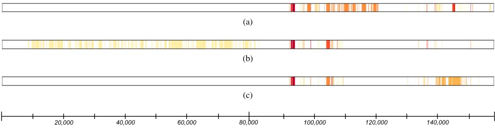
Figure 1 provides a visual depiction of these results for the blepharitis phenotype model. Among the 1,093 base features and feature groups that were tested, we determine that 107 are important when controlling the FDR atq= 0.05. More-over the set of 40 outer nodes represents the finest level of resolution at which we can say that a viral genomic region is important to the phenotype. In the case of the blephar-itis phenotype, six of the outer nodes are feature groups which represent genomic regions that seem to be associated with the phenotype but for which we cannot localize pre-cisely which base features are important. Figure 2 shows the identified important features for all three disease phe-notypes mapped to the genomic coordinates of the virus. Through the application of our approach to the learned RF models, we are able to significantly narrow down the ge-netic determinants of disease from a large number of can-didate regions. Several of these regions recapitulate what was previously known about HSV-1 pathogenicity, and oth-ers indicate novel disease determinants (Kolb et al. 2016; Lee et al. 2016). Moreover, the results suggest a high degree of underlying causality among the three disease phenotypes given the fact that there is substantial overlap among the important regions identified.
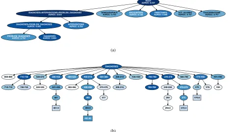
Figure 3a shows the results of our feature importance anal-ysis when applied to the highest level feature groups for the asthma-exacerbation model. These results suggest that the most informative feature groups are coded diagnoses (DIAGNOSES), intervals between events (TIMESTAMPS), and interventions (which combines medications and proce-dures). We note that even when all the features are erased (ROOT), the model still has some predictive power with AU-ROC = 0.537. This is likely due to the fact that the number of encounters in a patient’s history is predictive. Even when we erase all other information, we leave the number of events in a patient’s history intact. Figure 3b partially depicts the results of our hierarchical FDR analysis on the diagnosis fea-ture group. These results are also summarized in Table 2. A large number of hypotheses are rejected at FDR control level
HSV-1 genotype-phenotype association asthma exacerbation
blepharitis stromal keratitis neovascularization ICD-9
total nodes (base features + feature groups) 1,093 1,093 1,093 8,740
nodes with unadjustedp<0.05 242 148 111 3,480
nodes rejected atqlevel<0.05 107 110 80 3,179
outer nodes 40 36 24 2,120
feature groups among outer nodes 6 3 3 159
Table 2: Summary of feature-importance hypothesis testing in both application domains.
145 413 35 19 33 123 3 7 5 3 7 3 7 3 3 3 5 3 15
Figure 1: Feature importance analysis of the random forest model for blepharitis. Ovals represent feature groups, squares depict base features, and triangles depict subtrees of the hierarchy that were not tested by the FDR procedure. Color intensity indicates the magnitude of the associatedp-value. White nodes are those that were tested but did not survive the FDR procedure.
(a)
(b)
(c)
20,000 40,000 60,000 80,000 100,000 120,000 140,000
ROOT AUROC: 0.537
DIAGNOSES+INTERVENTIONS+PROBLEM_DIAGNOSES
AUROC: 0.623 DEMOGRAPHICSAUROC: 0.753 ENCOUNTERSAUROC: 0.728 AUROC: 0.696TIMESTAMPS ACT_SCORESAUROC: 0.757 EXACERBATIONSAUROC: 0.757
DIAGNOSES+PROBLEM_DIAGNOSES
AUROC: 0.663 INTERVENTIONSAUROC: 0.700
PROBLEM_DIAGNOSES
AUROC: 0.752 AUROC: 0.664DIAGNOSES
(a)
DIAGNOSES
800-999 710-739 520-579 390-459 580-629 460-519 320-389 290-319 V20-V29 780-799 240-279 680-709 V70-V82 V01-V06
710-719 720-724 530-539 401-405
401
401.9
460-466 490-496 470-478
493
493.9
493.90
477
300-316 780-789 249-259 270-279
250
250.0
272
272.4
V70 V76
V70.0
V04
(b)
Figure 3: Feature importance analysis of the LSTM model for predicting asthma exacerbations. Darker shades correspond to larger effect sizes (lower AUROCs when the feature groups are perturbed). (a) Importance analysis for highest level feature groups. (b) Importance analysis for feature groups representing the ICD-9 hierarchy of diagnoses. Note that the root node in panel (b) corresponds to theDIAGNOSESnode in panel (a).
sizes. The features identified by the analysis as important include those with known connections to asthma, such as therespiratory diseasessubtree (460-519) terminating at
asthma(493.90), and themental disorderssubtree (290-319) (Scott et al. 2007). It also identifies important features with less well understood relationships to asthma, such as the
metabolic diseasessubtree (240-279).
Identifying Important Interactions
We also apply our approach for detecting important fea-ture interactions to the models learned for HSV-1 genotype-phenotype associations. We have not yet developed an ap-proach for effectively exploring the space of hypotheses cor-responding to interactions while controlling the FDR, so here we evaluate interactions among two sets. First, we assess pairwise interactions between all outer nodes that were deter-mined as important in the individual feature analysis. There are 780, 630, and 276 pairwise interaction candidates to be tested by our approach for blepharitis, stromal keratitis, and neovascularization, respectively. After applying our hypothe-sis testing method for interactions to the outer nodes, we use the Benjamini-Hochberg method (1995) to control the false discovery rate among this set. Controlling FDR at 0.1, there is only one surviving interaction among the three phenotype models. For stromal keratitis, we identified a significant inter-action between two base features, where one of the features
is the one with the largest effect size among the outer nodes. We also consider interactions among a set of nodes located at an intermediate level in the hierarchy of features that sur-vived FDR control in the individual feature importance anal-ysis. We were able to detect several significant interactions for the stromal keratitis phenotype. Among 435 candidate interactions tested, three interactions were significant.
Conclusion
the importance of time-based feature groups in the context of our asthma exacerbation model, and analyzing feature groups that are organized into graphs that are not necessarily trees.
Acknowledgments
This work was funded by NIH grants U54 AI117924 and UL1 TR000427.
References
Alvarez-Melis, D., and Jaakkola, T. 2017. A causal framework for explaining the predictions of black-box sequence-to-sequence mod-els. InProceedings of the 2017 Conference on Empirical Methods in Natural Language Processing, 412–421. ACL Press.
Bau, D.; Zhou, B.; Khosla, A.; Oliva, A.; and Torralba, A. 2017. Network dissection: Quantifying interpretability of deep visual rep-resentations. InProceedings of the IEEE Conference on Computer Vision and Pattern Recognition, 3319–3327. IEEE.
Benjamini, Y., and Hochberg, Y. 1995. Controlling the false dis-covery rate: A practical and powerful approach to multiple testing. Journal of the Royal Statistical Society, Series B57(1):289–300. Bojarski, M.; Yeres, P.; Choromanska, A.; Choromanski, K.; Firner, B.; Jackel, L.; and Muller, U. 2017. Explaining how a deep neu-ral network trained with end-to-end learning steers a car. arXiv 1704.07911.
Breiman, L. 2001. Random forests.Machine Learning45(1):5–32. Choi, E.; Bahadori, M. T.; Searles, E.; Coffey, C.; Thompson, M.; Bost, J.; Tejedor-Sojo, J.; and Sun, J. 2016. Multi-layer represen-tation learning for medical concepts. InProceedings of the 22nd ACM SIGKDD International Conference on Knowledge Discovery and Data Mining, 1495–1504. ACM.
Craven, M., and Shavlik, J. 1996. Extracting tree-structured repre-sentations of trained networks. In Touretzky, D.; Mozer, M.; and Hasselmo, M., eds.,Advances in Neural Information Processing Systems, volume 8. MIT Press. 24–30.
Epifanio, I. 2017. Intervention in prediction measure: A new approach to assessing variable importance for random forests.BMC Bioinformatics18:230.
Fabris, F.; Doherty, A.; Palmer, D.; de Magalhaes, J.; and Freitas, A. 2018. A new approach for interpreting random forest models and its application to the biology of ageing.Bioinformatics34(14):2449– 2456.
Fong, R. C., and Vedaldi, A. 2017. Interpretable explanations of black boxes by meaningful perturbation. InProceedings of the IEEE Conference on Computer Vision and Pattern Recognition, 3429–3437. IEEE.
Friedman, J., and Popescu, B. 2008. Predictive learning via rule ensembles.Annals of Applied Statistics2:916–954.
Friedman, J. 2001. Greedy function approximation: A gradient boosting machine.Annals of Statistics5:1189–1232.
Hara, S., and Hayashi, K. 2018. Making tree ensembles inter-pretable: A Bayesian model selection approach. InProceedings of the Twenty-First International Conference on Artificial Intelligences and Statistics, 77–85. PMLR.
Hochreiter, S., and Schmidhuber, J. 1997. Long short-term memory. Neural Computation9(8):1735–1780.
Karpathy, A.; Johnson, J.; and Fei-Fei, L. 2016. Visualizing and understanding recurrent networks. InProceedings of the Fourth International Conference on Learning Representations.
Koh, P. W., and Liang, P. 2017. Understanding black-box predic-tions via influence funcpredic-tions. InProceedings of the International Conference on Machine Learning, 1885–1894. PMLR.
Kolb, A.; Lee, K.; Larsen, I.; Craven, M.; and Brandt, C. 2016. Quantitative trait locus based virulence determinant mapping of the HSV-1 genome in murine ocular infection: genes involved in viral regulatory and innate immune networks contribute to virulence. PLoS Pathogens12(3):e1005499.
Lee, K.; Kolb, A.; Larsen, I.; Craven, M.; and Brandt, C. 2016. Mapping murine corneal neovascularization and weight loss viru-lence determinants in the herpes simplex virus 1 genome and the detection of an epistatic interaction between the UL and IRS/US regions.Journal of Virology90(18):8115–8131.
Lei, T.; Barzilay, R.; and Jaakkola, T. 2016. Rationalizing neural predictions. InProceedings of the 2016 Conference on Empirical Methods in Natural Language Processing, 107–117. ACL Press. Leino, K.; Sen, S.; Datta, A.; Fredrikson, M.; and Li, L. 2018. Influence-directed explanations for deep convolutional networks. arXiv1802.03788.
Li, J.; Monroe, W.; and Jurafsky, D. 2016. Understanding neural networks through representation erasure. arXiv1612.08220. Lou, Y.; Caruana, R.; Hooker, G.; and Gehrke, J. 2013. Accurate intelligible models with pairwise interactions. InProceedings of the Nineteenth ACM SIGKDD International Conference on Knowledge Discovery and Data Mining, 623–631. ACM Press.
Miotto, R.; Li, L.; Kidd, B. A.; and Dudley, J. T. 2016. Deep patient: an unsupervised representation to predict the future of patients from the electronic health records.Scientific Reports6:26094.
Pham, T.; Tran, T.; Phung, D.; and Venkatesh, S. 2016. Deepcare: A deep dynamic memory model for predictive medicine. In Pacific-Asia Conference on Knowledge Discovery and Data Mining, 30–41. Springer.
Ribeiro, M.; Singh, S.; and Guestrin, C. 2016. Why should I trust you? Explaining the predictions of any classifier. InProceedings of the Twenty-Second ACM SIGKDD International Conference on Knowledge Discovery and Data Mining, 1135–1144. ACM Press. Ribeiro, M.; Singh, S.; and Guestrin, C. 2018. Anchors: High-precision model-agnostic explanations. InProceedings of the Thirty-Second AAAI Conference on Artificial Intelligence. AAAI Press. Scott, K. M.; Korff, M. V.; Ormel, J.; Zhang, M.; Bruffaerts, R.; Alonso, J.; Kessler, R. C.; Tachimori, H.; Karam, E.; Levinson, D.; et al. 2007. Mental disorders among adults with asthma: results from the world mental health survey.General Hospital Psychiatry 29(2):123–133.
Wan, C., and Freitas, A. 2018. An empirical evaluation of hierar-chical feature selection methods for classification in bioinformatics datasets with gene ontology-based features.Artificial Intelligence Review50:201–240.