Learning Disentangled Representation with Pairwise Independence

The Thirty-Third AAAI Conference on Artificial Intelligence (AAAI-19)

Learning Disentangled Representation with Pairwise Independence

Zejian Li,

Yongchuan Tang,

Wei Li,

Yongxing He

1_{College of Computer Science, Zhejiang University, Hangzhou 310027, China}

2_{Zhejiang Lab, Hangzhou 310027, China}

{zejianlee, yctang, liwei 2014, heyongxing_}@zju.edu.cn

Abstract

Unsupervised disentangled representation learning is one of the foundational methods to learn interpretable factors in the data. Existing learning methods are based on the assumption that disentangled factors are mutually independent and incor-porate this assumption with the evidence lower bound. How-ever, our experiment reveals that factors in real-world data tend to be pairwise independent. Accordingly, we propose a new method based on a pairwise independence assumption to learn the disentangled representation. The evidence lower bound implicitly encourages mutual independence of latent codes so it is too strong for our assumption. Therefore, we introduce another lower bound in our method. Extensive ex-periments show that our proposed method gives competitive performances as compared with other state-of-the-art methods.

1

Introduction

This paper is concerned with the unsupervised learning of disentangled representation. The disentangled representation is a distributed data representation in which latent codes represent interpretable attributes. Disjoint dimensions of the representation change independently in the variation of the data and are associated with different high-level data fac-tors (Bengio, Courville, and Vincent 2013). One example of the disentangled representation is the task of generating hand-written digits. The hand-written digits are generated by the generator according to the latent codes, while different codes control rotation, stroke width, writing style and other different attributes. These attributes interact non-linearly in the data. However, when one factor varies but all others are fixed, the generated sequence of samples can show an interpretable change to human beings. Due to its interpretabil-ity, disentangled representations are useful in many down-stream tasks such as supervised learning (Liu et al. 2018; Hadad, Wolf, and Shahar 2018) and transfer learning (Zamir et al. 2018).

Many recent works have been devoted to the super-vised learning of disentangled representation. Bouchacourt, Tomioka, and Nowozin (2018) and Hadad, Wolf, and Sha-har (2018) assume the group division of samples is given. Liu et al. (2018) require the predefined attributes. Adel,

∗

Corresponding author

Copyright c2019, Association for the Advancement of Artificial Intelligence (www.aaai.org). All rights reserved.

Ghahramani, and Weller (2018) consider side information in the learning process. However, real-world data is often raw data without labels or attributes, and thus the unsuper-vised learning of disentangled representation is an important and challenging problem. Most existing methods are based on the prior assumption that the learned codes should be mutually independent. It is believed that interpretable fac-tors tend to change independently in the data, so by infer-ring independent codes, the model may capture those in-terpretable factors backward. To model this independence, Higgins et al. (2017) and Burgess et al. (2018) limit the capacity of learning model. Kumar, Sattigeri, and Balakr-ishnan (2018) match the code distribution to the standard normal distribution. Kim and Mnih (2018) and Chen et al. (2018) optimize the term of total correlation to enable the distribution to be factorial. Other works (Chen et al. 2016; Li, Tang, and He 2018) take the principle of mutual informa-tion minimizainforma-tion. Most of these methods are built on top of variational autoencoder (Kingma and Welling 2014).

However, we find interpretable factors are pairwise inde-pendent in experiments. We perform Pearson’s chi-squared test on the CelebA attributes (Liu et al. 2015) and find that some attributes pairs are independent. However, only a group of three attributes is three-wise independent and no four-wise independent group is observed. Therefore, we assume the latent codes of data are pairwise independence in the design of our model. Notice that pairwise independence is different

from mutual independence. A finite set ofkrandom

vari-ables_{Z1, . . . , Zk}are pairwise independent when any two

of them are independent. However, they are mutually inde-pendent only when the joint cumulative distribution function is always the product of the marginal cumulative functions,

namelyFZ1,...,Zk(z1, . . . , zk) =

Qk

i=1FZi(zi). Since

mu-tual independence is a special case of pairwise independence, our assumption is more general.

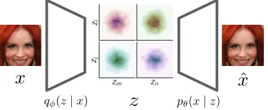
of the joint distribution of the latent code. As a result, it can incorporate the pairwise independence assumption which constrains the joint distribution between code pairs. Finally, the discussed lower bound is combined with a designed pair-wise independence term. Inspired by (Kingma and Welling 2014), our model is implemented with deep neural networks and trained with the stochastic optimization method and the reparameterization trick. Figure 1 shows an illustration of our model.

x

x

ˆ

z

q (z|x) p✓(x_|z)

Figure 1:The architecture of our proposed method.Given

a samplex, the encoderqφ(z|x)infers the codezand the

de-coderpθ(x|z)recoversxˆaccordingly. The aggregated

poste-rior distributionqφ(z)is encouraged to be pairwise

indepen-dent. To illustrate the idea, we visualize the pairwise joint

dis-tributions ofqφ(z). Herezi, zj, zmandznare different code

components. Ideally we have qφ(zi, zm) = qφ(zi)qφ(zm)

and the same holds for other code pairs. The notations are summarized in Table 1. The figure is best viewed magnified on screen.

An outline of the remainder of our paper is as follows. Section 2 gives a brief review of related works. Section 3 describes our experiments on CelebA attributes and shows the attributes tend to be pairwise independent. Based on this observation, Section 4 introduces our proposed model, which combines our discussed lower bound and the de-signed term to measure pairwise independence. In Sec-tion 5, we perform canonical correlaSec-tion analysis between the CelebA attributes and the learned codes of different mod-els to show how well the methods capture the attributes. Finally, Section 6 concludes our paper. Our source code is available on https://github.com/ZejianLi/Pairwise-Indepence-Autoencoder.

2

Related Works

In this part, we give a brief introduction of variational au-toencoder (Kingma and Welling 2014) and its variants which learn disentangled representations.

Variational autoencoder (VAE) has been a foundational generative model to learn the latent representation. Given

ak-dimensional latent code z _{∈ Z} sampled from a prior

distributionp(z), a new samplex _{∈ X} can be generated

withpθ(x|z). To increase the log-likelihood of the observed

sampleslogpθ(x), VAE maximizes the evidence lower bound

(ELBO) (Jordan et al. 1999) defined as:

L(θ, φ) =Ep(x)Eqφ(z|x)log

pθ(x, z)

qφ(z|x) ≤Ep(x)

logpθ(x). (1) The notations are summarized in detail in Table 1.

Table 1: Notations.

Notation Definition

x An observed sample from the data space_X.

z A code in thek-dimensional latent space_Z.

p(x) The ground-truth data distribution ofx,

as-sumed to be absolutely continuous.

p(z) The prior distribution ofz, assumed to be

N(0, I).

pθ(x|z) The distribution to generate a new sample

xgivenz, parameterized byθ.

pθ(x) The marginal distribution of pθ(x, z) =

p(z)pθ(x|z).

qφ(z|x) The variational distribution of the posterior

pθ(z|x), parameterized byφ.

qφ(z) The marginal distribution of qφ(x, z) =

p(x)qφ(z|x).

B A mini-batch ofbsamples_{x1, . . . , xb}.

VAE can disentangle factors by encouraging the latent codes to be independent (Hoffman and Johnson 2016). To see this, the ELBO is decomposed as:

Ep(x)Eqφ(z|x)log

pθ(x, z) qφ(z|x)

=Ep(x)Eqφ(z|x)logpθ(x|z)−Eqφ(z,x)log

qφ(z|x) p(z) .

(2) The first term is the expected log-likelihood to recover the

samplex. The second term can be further decomposed as:

Eqφ(z,x)log

qφ(z|x) p(z) =Eqφ(z,x)log

qφ(z, x) qφ(z)p(x)

+Eqφ(z)log

qφ(z) p(z) =Iφ(z;x) + KL(qφ(z)kp(z)).

(3)

Iφ(z;x)is the mutual information betweenxandzspecified

byqφ(z, x).KL(qφ(z)kp(z))is the Kullback-Leibler

diver-gence betweenqφ(z)andp(z). It guidesqφ(z)to be factorial

and the marginal distributions ofqφ(z)to be Gaussian. To

see this,KL(qφ(z)kp(z))is decomposed as

KL(qφ(z)kp(z))

=Eqφ(z)log

qφ(z)

Qk

i=1qφ(zi) +

k X

i=1

Eqφ(zi)log

qφ(zi) p(zi)

. (4)

Eqφ(z)log

qφ(z)

Qk

i=1qφ(zi) is the total correlation of the latent

codes. Similar to mutual information, the total correlation

is zero whenqφ(zi)fori= 1, . . . , kare mutually

indepen-dent. Therefore, VAE encourages the independence of la-tent codes and thus disentangles the generative factors. Re-cent works are mainly focused on putting more emphasis on

the independence. Specifically,β-VAE (Higgins et al. 2017;

Burgess et al. 2018) put more weight onEqφ(z,x)log

qφ(z|x)

p(z)

in (2) and thus penalize the total correlation term.

5_o_Clock_Shadow Arched_Eyebrows

Attractive

Bags_Under_Eyes

Bald Bangs

Big_Lips Big_Nose Black_Hair Blond_Hair Blurry _{Brown_Hair}

Bushy_Eyebrows

Chubby

Double_Chin Eyeglasses

Goatee

Gray_Hair

Heavy_Makeup

High_Cheekbones

Male

Mouth_Slightly_Open

Mustache

Narrow_Eyes No_Beard Oval_Face Pale_Skin Pointy_Nose

Receding_Hairline

Rosy_Cheeks Sideburns

Smiling

Straight_Hair Wavy_Hair

Wearing_Earrings

Wearing_Hat

Wearing_Lipstick Wearing_Necklace Wearing_Necktie

Young

5_o_Clock_Shadow Arched_Eyebrows Attractive Bags_Under_Eyes Bald Bangs Big_Lips Big_Nose Black_Hair Blond_Hair Blurry Brown_Hair Bushy_Eyebrows Chubby Double_Chin Eyeglasses Goatee Gray_Hair Heavy_Makeup High_Cheekbones Male Mouth_Slightly_Open Mustache Narrow_Eyes No_Beard Oval_Face Pale_Skin Pointy_Nose Receding_Hairline Rosy_Cheeks Sideburns Smiling Straight_Hair Wavy_Hair Wearing_Earrings Wearing_Hat Wearing_Lipstick Wearing_Necklace Wearing_Necktie Young

0.0 0.2 0.4 0.6 0.8 1.0

P-value

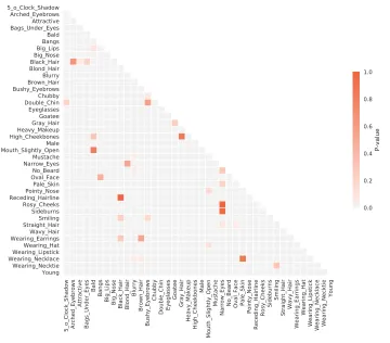
Figure 2:The p-values in the Pearson’s chi-squared test on the attribute pairs of CelebA dataset.It is observed that36

pairs are not significantly dependent with a significant level of0.01. The figure is best viewed on screen.

al. 2018) augment the ELBO with the total correlation term directly. Similarly, DIP-VAE (Kumar, Sattigeri, and Balakrishnan 2018) designs an moment-matching term to

minimizeKL(qφ(z)kp(z))in (3). The assumption behind

VAE and these variants is that interpretable factors are mutually independent and can be captured with the

fac-torial distribution p(z). Other works (Chen et al. 2016;

Li, Tang, and He 2018) encourage disentanglement by

mini-mizing the mutual information betweenxandzwith extra

components of the model.

3

Experiment on CelebA Attributes

We tentatively argue that the interpretable factors may be pairwise independent, but not mutually independent. Our argument is supported by the following experiment findings. We conduct the Pearson’s chi-squared test on the labeled

attributes of CelebA dataset (Liu et al. 2015). These40

at-tributes are binary and concerned with different aspects of the faces. Notice that some attributes are intrinsically correlated, such as “brown hair” and “black hair”, or “narrow eyes” and “smiling”. Firstly, we perform the test on attribute pairs and

find36pairs are not significantly dependent with a significant

level of0.01. The p-values of all pairwise tests are visualized

in Figure 2. We also perform the test on groups of three and four attributes. Only the group of “Blond Hair”, “Straight

Hair” and “Narrow Eyes” is not significantly dependent with

the p-value as0.038, and all groups of four attributes are

significantly dependent. So in this experiment, attributes in CelebA dataset are not mutually independent while some attribute pairs are independent.

The assumption of mutual independence may be too strong and interpretable factors in the real-world data tend to be pair-wise independent. Intuitively, human beings can easily see whether two factors are independent or not, but mutual inde-pendence among three or more factors is not straightforward.

Given three factorsA,B andC, one should first consider

they are pairwise independent or not and then investigate

whetherAand the joint distribution of(B, C)are

indepen-dent. The latter investigation is involved with high-order relations between factors, which is not intuitive. However, most interpretable factors are intuitive and come easily from common sense. Therefore, we hypothesize that pairwise inde-pendent factors may be more consistent with human intuition. Our proposed method is based on the assumption of pairwise independence.

4

Method

describe our method to approximate the pairwise indepen-dence of latent codes. We also derive a variant of ELBO, which does not contain the total correlation term and con-strains only the marginal distributions of the latent codes. Our proposed method combines the derived lower bound with the term of pairwise independence.

Given two code componentsziandzjwherei=6 j,qφ(zi)

andqφ(zj)are expected to be independent in our scenario.

The independence is measured by the mutual information

Iφ(zi;zj) =Eqφ(zi,zj)log

qφ(zi, zj) qφ(zi)qφ(zj)

.

To approximateqφ(zi), we use the Monte Carlo estimation

based on a mini-batch of samples_Bfromp(x). Since the

aggregated posteriorqφ(z) =Ep(x)qφ(z|x),qφ(z)can be

approximated by 1_bPb

l=1qφ(z |xl), which is a mixture of

Gaussian distributions asqφ(z|xl)isN(µφ(xl), σφ2(xl)I).

To sample fromqφ(zi), we first choose a samplexlfromB

uniformly at random. Next we use the reparameterization

trick and havez˜i=µφ,i(xl) +σφ,i(xl)where∼ N(0, I).

Then we have the estimatorqφ(˜zi) = 1_bPlb=1qφ(˜zi | xl).

The same estimation can be applied toqφ(zj)andqφ(zi, zj),

too. This estimation is acceptable in our scenario because it is in the one-dimensional or two-dimensional space, and those high-dimensional sampling problems discussed in (Chen et al. 2018; Kim and Mnih 2018) are avoided. We define the average mutual information of code pairs as

P I1(qφ(z)) =

1

k

2

X

i6=j

Iφ(zi;zj). (5)

An alternative measure of the pairwise independence is the KL-divergence between the aggregated posterior and the prior, defined as

KL(qφ(zi, zj)kp(zi, zj))

=Eqφ(zi,zj)log

qφ(zi, zj) p(zi, zj)

=Iφ(zi;zj) + KL(qφ(zi)kp(zi)) + KL(qφ(zj)kp(zj)). This consists of the mutual information and the

KL-divergences which pushqφ(zi)top(zi)andqφ(zj)top(zj).

Additionally, this is more computationally efficient because

it eliminates the computation ofqφ(˜zi)andqφ(˜zj)and only

requires the probability ofqφ(˜zi,z˜j)andp(˜zi,z˜j). Thus, we

define

P I2(qφ(z)) =

1

k

2

X

i6=j

KL(qφ(zi, zj)kp(zi, zj)). (6)

It is not appropriate to combine the pairwise independence term with the ELBO. The ELBO contains the total correlation term and encourages mutual independence of codes, so it is too strong for the pairwise independence assumption. We introduce a different lower bound based on variational infer-ence and design a corresponding autoencoding framework.

We rewrite the expected log-likelihood as:

Ep(x)logpθ(x)

=Ep(x)Eqφ(z|x)log

pθ(z, x) pθ(z|x)

=Eqφ(z,x)logpθ(z, x)−Ep(x)Eqφ(z|x)logpθ(z|x).

The second term is the expected cross entropy over the

random variablezgivenx, denoted asH(qφ(z|x), pθ(z |

x)). With Jensen’s inequality, we have

H(qφ(z|x), pθ(z|x))≥H(qφ(z|x)),

whereH(qφ(z|x))is the differential entropy ofz. Notice

that the differential entropy can be negative. However, when

H(qφ(z|x))is non-negative, we have

H(qφ(z|x), pθ(z|x))≥0

and thus_L0(θ, φ) =Eqφ(z,x)logpθ(z, x)is a lower bound of

the log-likelihood. The bound is tight whenH(qφ(z|x)) =

0andqφ(z|x)matchespθ(z|x).

To analyze_L0(θ, φ), we decompose it into two parts.

L0_{(θ, φ) =}

Eqφ(z,x)logpθ(x|z) +Eqφ(z)logp(z)

=Ep(x)Eqφ(z|x)logpθ(x|z) +

k X

i=1

Eqφ(zi)logp(zi).

We havelogp(z) =Pk

i=1logp(zi)becausep(z)isN(0, I).

The first term is the log-likelihood that pθ(x | z)

recov-ers sample x given the latent code from qφ(z | x). The

second term is the sum of the negative cross entropies −H(qφ(zi), p(zi))fori= 1, . . . , k. It restricts the marginal

distributionsqφ(zi)instead of the joint distributionqφ(z).

Finally, we augment_L0(θ, φ)with the pairwise

indepen-dence term and arrive at the optimization problem of our Pairwise Independence Autoencoder (PIAE) as follows:

arg max

θ,φ L

0_{(θ, φ)}

−λPIα(qφ(z)),

s.t. H(qφ(z|x))≥0 forx∈ X.

(7)

Hereλis the penalty parameter. When we haveα= 1and

takePI1(qφ(z))in (5), we term our model as PIAE(MI). MI

is short for mutual information. Similarly, we have PIAE(KL)

when taking (6) withα= 2.

To make the optimization easier,qφ(z|x)is assumed to

be_N(µφ(x), σ2φ(x)I). The model is trained with stochastic

batches with the reparameterization trick. Notice that the

differential entropy ofqφ(z|x)is

H(qφ(z|x)) =

1

2ln det|2πeσ 2

φ(x)|

=1 2

k X

i=1

ln(2πeσ2

φ,i(x)).

H(qφ(z | x)) ≥ 0 whenln(2πeσφ,i2 (x)) ≥ 0 for any i,

which is equivalent toσ2

φ,i(x)≥

1

2πe ≈0.0585. To model

this constraint,σ2

φ(x) is defined asmax(fφ(x),0) + ₂1_πe,

Unfortunately, the proposed method does not have the ability to generate high-quality new samples. This is because

qφ(z)is unknown and may lie in a low-dimensional manifold

due to the pairwise independence constraint. Thus, codes

sampled fromp(z)may be out of the support ofqφ(z).

We further show that the lower bound_L0(θ, φ)is closely

related to rate-distortion theory (Cover and Thomas 2006). We begin with the following optimization

maxEqφ(z)logp(z)

s.t. ₋Eqφ(z,x)logpθ(x|z)≤D.

(8)

Dis a constant. Writing (8) as a Lagrangian we have

L0_{(θ, φ, β) =}

Eqφ(z)logp(z) +βEqφ(z,x)logpθ(x|z).

L0_{(θ, φ)is a special case whenβ= 1. (8) has a close relation}

with the rate-distortion function. AsH(qφ(z|x)≥0,

Eqφ(z)logp(z)≤Eqφ(z,x)logp(z) +Ep(x)H(qφ(z|x))

=₋Eqφ(z,x)log

qφ(z|x) p(z) ≤ −Iφ(z;x).

In the last step we use (3) and that KL-divergence is

non-negative. Thus the mutual informationIφ(z;x)is minimized

whenEqφ(z)logp(z)is maximized. On the other hand, when

pθ(x|z)isN(µθ(z), I), we have

−Eqφ(z,x)logpθ(x|z) =Eqφ(z,x)

kµθ(z)−xk2

2 +C

,

whereCis a constant. Thus₋Eqφ(z,x)logpθ(x| z)

corre-sponds to the squared-error distortion. To summarize, (8) is related to the following rate-distortion function

R(D0) = minIφ(x;z)

s.t.Eqφ(z,x)kµθ(z)−xk

2 ≤D0,

whereD0 _{= 2(D}

−C). Therefore, the optimization in (8)

helps the model to find an achievable rate and distortion pair so as to learn a useful representation for reconstruction. This

is the same for_L0(θ, φ).

5

Experiment

In this section, we compare our proposed methods with other state-of-the-art methods. Particularly, we compare how well the methods capture the attributes in CelebA dataset by ex-amining the maximum correlations and the prediction perfor-mances in canonical correlation analysis. We also compare the methods along subspace score (Li, Tang, and He 2018), an unsupervised disentanglement metric. Furthermore, we display rerendered sample sequences in the latent traversal as appropriate. The experiments are conducted on several image datasets, including MNIST (LeCun et al. 1998), Fash-ionMNIST (Xiao, Rasul, and Vollgraf 2017), CelebA (Liu et al. 2015), Flower (Nilsback and Zisserman 2008), CUB (Wah et al. 2011), Chairs (Aubry et al. 2014) and CIFAR10 (Krizhevsky, Nair, and Hinton 2009).

Methods to be compared includeβ-VAE (β = 20)

(Hig-gins et al. 2017), Improvedβ-VAE (β = 30) (Burgess et al.

2018), DIP-VAE (λ = 20) (Kumar, Sattigeri, and

Balakr-ishnan 2018),β-TCVAE (β = 20) (Chen et al. 2018) and

FactorVAE (γ= 20) (Kim and Mnih 2018). These are

meth-ods based on the mutual independence assumption. We also include comparisons with AnaVAE (Li, Tang, and He 2018) and InfoGAN (Chen et al. 2016). VAE (Kingma and Welling 2014) is also compared as a baseline. Hyperparameters are

chosen as suggested in the original papers. We setλ= 20in

(7) for our PIAE(MI) and PIAE(KL).

We does not perform comparisons along the disentangle-ment metrics proposed in (Higgins et al. 2017; Kim and Mnih 2018; Chen et al. 2018) in our experiments. These metrics are applied on the synthetic dataset of 2D shapes (Matthey et al. 2017), whose factors are defined to be mutual independent. Therefore, they are not applicable in our scenario.

Implementation Details

Implementation details of our models are summarized here.

The latent dimension ofzis set as16in MNIST and

Fashion-MNIST, and64in other datasets. The network architecture is

designed according to DCGAN (Radford, Metz, and Chintala 2015). Specifically, the encoder borrows the major structure of the discriminator in DCGAN and the decoder is the same as the generator. The architecture guidelines introduced in (Radford, Metz, and Chintala 2015) can make the training easier and more stable. We use Adam optimizer (Kingma

and Ba 2014) with a learning rate of0.0001and a

momen-tum of0.5. The batch size is64. Different from the notation

in (5) and (6), we randomly select onlyk₋1 pairs ofzi

andzj in each batch to reduce the computational cost. In

the whole training process, all code pairs are constrained. Empirically, this stochastic approximation shows acceptable performance, but its robustness remains unclear and will be studied in our future work. Finally, the proposed algorithms are implemented with PyTorch (Paszke et al. 2017).

Canonical Correlation Analysis

To evaluate the learned code, we analyze the relation

be-tween the codezand the attributesyannotated in CelebA

dataset. Inspired by (Adel, Ghahramani, and Weller 2018), we hypothesize that in the ideal case this relation can be described by a linear model. We use canonical correlation analysis (CCA) because CelebA attributes are correlated. The evaluation framework (Eastwood and Williams 2018) applies individual least square estimate for each attribute, implicitly assuming the attributes are uncorrelated, so it is not appli-cable here. Instead, CCA finds a sequence of uncorrelated

linear combinations zvm form = 1, . . . ,40and a

corre-sponding sequence of uncorrelatedyumsuch that the

corre-lationsCorr(zvm, yum)’s are successively maximized. The

leading canonical responses are those linear combinations of attributes best predicted by the codes. By investigating the leading correlation coefficients, we can see how well the attributes are captured.

Table 2:Four leading correlation coefficients in the CCA analysis. The best performances are highlighted.

Training set Testing set

1 2 3 4 1 2 3 4

VAE 0.890 0.826 0.705 0.697 0.890 0.826 0.704 0.697

InfoGAN 0.374 0.314 0.147 0.101 0.373 0.313 0.146 0.099

β-VAE 0.751 0.729 0.649 0.648 0.751 0.729 0.647 0.649

Improvedβ-VAE 0.728 0.705 0.642 0.627 0.728 0.705 0.641 0.626

DIP-VAE 0.866 0.801 0.756 0.707 0.866 0.801 0.756 0.707

β-TCVAE 0.755 0.725 0.697 0.663 0.754 0.724 0.696 0.663

FactorVAE 0.884 0.825 0.721 0.693 0.883 0.825 0.720 0.693

AnaVAE 0.893 0.826 0.710 0.693 0.893 0.826 0.709 0.693

PIAE(MI) 0.892 0.830 0.716 0.695 0.891 0.829 0.716 0.695

PIAE(KL) 0.890 0.828 0.717 0.692 0.890 0.827 0.716 0.692

the codes capture the attributes. For the first correlation co-efficients, AnaVAE has the largest values and our methods have marginally smaller ones. For the second correlations, our methods have the highest values. For the third and forth correlations, DIP-VAE has the largest correlations. However, the first two correlations of DIP-VAE are significantly lower than those of other methods. Generally, our methods give competitive performances.

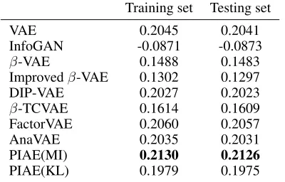
We also investigate the prediction accuracy in CCA. A higher accuracy means the model captures the attributes

bet-ter. The prediction accuracies are evaluated byR2_{score on}

the training and testing set, as shown in Table 3.R2 _score

can be negative since the performance can be arbitrary

inef-fective, and its best possible value is1. In this experiment,

our method gives the best performances in both cases.

Table 3:The averageR2 _{score in the CCA analysis.The}

best performances are highlighted.

Training set Testing set

VAE 0.2045 0.2041

InfoGAN -0.0871 -0.0873

β-VAE 0.1488 0.1483

Improvedβ-VAE 0.1302 0.1297

DIP-VAE 0.2027 0.2023

β-TCVAE 0.1614 0.1609

FactorVAE 0.2060 0.2057

AnaVAE 0.2035 0.2031

PIAE(MI) 0.2130 0.2126

PIAE(KL) 0.1979 0.1975

Subspace Score

In this part we present the comparison along subspace score (Li, Tang, and He 2018). Subspace score is an unsupervised disentanglement metric. It is based on two assumptions. The first one is that sample sequences generated by varying one latent code are expected to form an affine subspace, and subspaces of different latent codes are independent. This is measured by the clustering performance of a designed sub-space clustering method. The second is that the union of

these subspaces should be close to the majority of observed samples. This is reflected by the average distance between the samples and their projections in the subspace. The model with a higher subspace score is believed to separate indepen-dent factors better. Different from the implementation in (Li, Tang, and He 2018), we use the thresholding ridge regression (Peng, Yi, and Tang 2015) instead of orthogonal match pur-suit in the subspace clustering part, because the thresholding ridge regression method is robust in capturing subspaces and more computationally efficient. We calculate the subspace score over five different sets of generated samples to get the average.

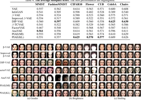
The results are shown in Table 4. DIP-VAE has the high-est score in FashionMNIST and CelebA dataset and has a slightly higher score than our method in Chairs. AnaVAE has the best performance in MNIST. PIAE(KL) enjoys the best performances in CIFAR10, Flower and CUB datasets. PIAE(MI) has similar performance. In summary, our methods have competitive performances in this experiment.

Latent Traversal

In this part, we present the latent traversal to show the learned factors. The latent traversal is conducted in the following way. Given a selected example, the encoder infers the code

z. Then a specific component ofzis varied, and accordingly

the decoder rerenders a sequence of samples. The variation of the sample sequences can visualize attributes learned by the autoencoding model.

Figure 3 shows the sample sequences of CelebA dataset. The models learn to disentangle factors including gender (a), the skin brightness (b) and the smiling of the face (c).

Theβ-VAE and its improved variant give blurry faces, while

Table 4:The average subspace score.The best performances are highlighted.

MNIST FashionMNIST CIFAR10 Flower CUB CelebA Chairs

VAE 0.557 0.562 0.614 0.563 0.571 0.600 0.608

InfoGAN 0.541 0.505 0.598 0.482 0.528 0.309 0.540

β-VAE 0.554 0.524 0.590 0.523 0.560 0.575 0.571

Improvedβ-VAE 0.554 0.517 0.589 0.522 0.551 0.572 0.561

DIP-VAE 0.560 0.597 0.609 0.560 0.558 0.625 0.630

β-TCVAE 0.541 0.522 0.582 0.529 0.540 0.565 0.586

FactorVAE 0.467 0.548 0.611 0.568 0.567 0.587 0.611

AnaVAE 0.561 0.556 0.614 0.561 0.571 0.596 0.611

PIAE(MI) 0.553 0.558 0.619 0.563 0.574 0.610 0.629

PIAE(KL) 0.551 0.557 0.625 0.570 0.577 0.609 0.626

PIAE(KL)

β-VAE

Improved

β-VAE

DIP-VAE

FactorVAE

AnaVAE

PIAE(MI)

(a) Gender (b) Brightness (c) Smiling

Figure 3:Latent factors learned in CelebA dataset.The pictures are generated by varying a component of the inferred code of

a selected input image. Each figure grid shows the variation of the similar factors, and each row shows the samples generated by the same method. The models learn to disentangle factors including gender (a), the skin brightness (b) and the smiling of the face (c). The pictures are best viewed magnified on screen.

seem to confuse brightness with skin color. The difference between these two factors is subtle in image data. On the

other hand,β-VAE and its variants give almost the

identi-cal sequences in grid (b), and they isolate brightness in a relatively clear way. They even infer the effect of overexpo-sure at the end of the sequences. In grid (c), our methods and DIP-VAE entangle the smiling factor with the factor of wearing lipsticks. In general, our methods give a comparable performance in separating disentangled factors.

6

Conclusion

In this paper, we propose our Pairwise Independence Autoen-coder with the attempt to learn unsupervised disentangled representation. Our method is motivated by our finding that attributes in the real-world dataset tend to be pairwise in-dependent rather than mutually inin-dependent. A variant of the evident lower bound is introduced, which requires the variational posterior to have a non-negative differential en-tropy and restricts only marginal distributions. Our proposed

models incorporate the lower bound with the terms of pair-wise independence. Experiments show that our models can uncover interpretable factors in the data and give compet-itive performances as compared with other state-of-the-art methods. However, we believe not all interpretable factors are pairwise independent, and some are even correlated. As shown in Figure 3, some factors are jointly represented by one code; correlated factors may not be disentangled with the independence prior without supervised signal. Further-more, the pairwise independence assumption may not be fully satisfied in real-world data. Therefore, we will explore the potential learning methods with a more general assumption.

Acknowledgments

References

Adel, T.; Ghahramani, Z.; and Weller, A. 2018. Discovering interpretable representations for both deep generative and

dis-criminative models. InInternational Conference on Machine

Learning (ICML), volume 80 of Proceedings of Machine Learning Research, 50–59. PMLR.

Aubry, M.; Maturana, D.; Efros, A. A.; Russell, B. C.; and Sivic, J. 2014. Seeing 3D chairs: exemplar part-based 2D-3D

alignment using a large dataset of CAD models. InIEEE

Conference on Computer Vision and Pattern Recognition (CVPR), 3762–3769. IEEE.

Bengio, Y.; Courville, A.; and Vincent, P. 2013.

Repre-sentation learning: A review and new perspectives. IEEE

transactions on pattern analysis and machine intelligence (TPAMI)35(8):1798–1828.

Bouchacourt, D.; Tomioka, R.; and Nowozin, S. 2018. Multi-level variational autoencoder: Learning disentangled

repre-sentations from grouped observations. InAAAI Conference

on Artificial Intelligence, 2095–2102.

Burgess, C. P.; Higgins, I.; Pal, A.; Matthey, L.; Watters, N.; Desjardins, G.; and Lerchner, A. 2018. Understanding

disentangling inβ-VAE. arXiv preprint arXiv:1804.03599.

Chen, X.; Duan, Y.; Houthooft, R.; Schulman, J.; Sutskever, I.; and Abbeel, P. 2016. InfoGAN: Interpretable representa-tion learning by informarepresenta-tion maximizing generative

adver-sarial nets. InAdvances in Neural Information Processing

Systems (NIPS), 2172–2180. Curran Associates, Inc. Chen, T. Q.; Li, X.; Grosse, R.; and Duvenaud, D. 2018. Iso-lating sources of disentanglement in variational autoencoders. arXiv preprint arXiv:1802.04942.

Cover, T. M., and Thomas, J. A. 2006.Elements of

Informa-tion Theory (2nd EdiInforma-tion). Wiley.

Eastwood, C., and Williams, C. K. I. 2018. A framework for the quantitative evaluation of disentangled

representa-tions. InInternational Conference on Learning

Representa-tion (ICLR).

Hadad, N.; Wolf, L.; and Shahar, M. 2018. A two-step

disentanglement method. InIEEE Conference on Computer

Vision and Pattern Recognition (CVPR), 772–780.

Higgins, I.; Matthey, L.; Pal, A.; Burgess, C.; Glorot, X.;

Botvinick, M.; Mohamed, S.; and Lerchner, A. 2017. β

-VAE: Learning basic visual concepts with a constrained

vari-ational framework. InInternational Conference on Learning

Representation (ICLR).

Hoffman, M. D., and Johnson, M. J. 2016. Elbo surgery: yet another way to carve up the variational evidence lower bound. InWorkshop in Advances in Approximate Bayesian Inference, Advances in Neural Information Processing Systems (NIPS). Jordan, M. I.; Ghahramani, Z.; Jaakkola, T. S.; and Saul, L. K. 1999. An introduction to variational methods for graphical

models.Machine learning37(2):183–233.

Kim, H., and Mnih, A. 2018. Disentangling by factorising. InInternational Conference on Machine Learning (ICML),

volume 80 ofProceedings of Machine Learning Research,

2654–2663. PMLR.

Kingma, D., and Ba, J. 2014. Adam: A method for

stochas-tic optimization. InInternational Conference on Learning

Representations (ICLR).

Kingma, D. P., and Welling, M. 2014. Auto-encoding

varia-tional bayes. InInternational Conference on Learning

Rep-resentation (ICLR).

Krizhevsky, A.; Nair, V.; and Hinton, G. 2009. Learning multiple layers of features from tiny images. Technical report, Department of Computer Science, University of Toronto. Kumar, A.; Sattigeri, P.; and Balakrishnan, A. 2018. Vari-ational inference of disentangled latent concepts from

unla-beled observations. InInternational Conference on Learning

Representation (ICLR).

LeCun, Y.; Bottou, L.; Bengio, Y.; and Haffner, P. 1998. Gradient-based learning applied to document recognition. Proceedings of the IEEE86(11):2278–2324.

Li, Z.; Tang, Y.; and He, Y. 2018. Unsupervised disentangled

representation learning with analogical relations. In

Inter-national Joint Conference on Artificial Intelligence (IJCAI), 2418–2424. International Joint Conferences on Artificial Intelligence Organization.

Liu, Z.; Luo, P.; Wang, X.; and Tang, X. 2015. Deep learning

face attributes in the wild. InInternational Conference on

Computer Vision (ICCV), 3730–3738. IEEE.

Liu, Y.; Wei, F.; Shao, J.; Sheng, L.; Yan, J.; and Wang, X. 2018. Exploring disentangled feature representation beyond

face identification. InIEEE Conference on Computer Vision

and Pattern Recognition (CVPR), 2080–2089.

Matthey, L.; Higgins, I.; Hassabis, D.; and Lerchner, A.

2017. dSprites: Disentanglement testing sprites dataset.

https://github.com/deepmind/dsprites-dataset/.

Nilsback, M.-E., and Zisserman, A. 2008. Automated flower

classification over a large number of classes. InIndian

Con-ference on Computer Vision, Graphics & Image, 722–729. IEEE.

Paszke, A.; Gross, S.; Chintala, S.; Chanan, G.; Yang, E.; DeVito, Z.; Lin, Z.; Desmaison, A.; Antiga, L.; and Lerer, A.

2017. Automatic differentiation in pytorch. InAutodiff

Work-shop, Advances in Neural Information Processing Systems (NIPS).

Peng, X.; Yi, Z.; and Tang, H. 2015. Robust subspace

clus-tering via thresholding ridge regression. InAAAI Conference

on Artificial Intelligence, 3827–3833.

Radford, A.; Metz, L.; and Chintala, S. 2015. Unsupervised representation learning with deep convolutional generative

adversarial networks. InInternational Conference on

Learn-ing Representation (ICLR).

Wah, C.; Branson, S.; Welinder, P.; Perona, P.; and Belongie, S. 2011. The caltech-ucsd birds-200-2011 dataset.

Xiao, H.; Rasul, K.; and Vollgraf, R. 2017. Fashion-MNIST: a novel image dataset for benchmarking machine learning algorithms.

Zamir, A. R.; Sax, A.; Shen, W.; Guibas, L. J.; Malik, J.; and Savarese, S. 2018. Taskonomy: Disentangling task

transfer learning. InIEEE Conference on Computer Vision