Continuous Time Control for Bilateral Telemetry Application

Fall 2018

Continuous Time Control for Bilateral Telemetry Application

Continuous Time Control for Bilateral Telemetry Application

Madhura Kulkarni

Iowa State University, [email protected]

Follow this and additional works at: https://lib.dr.iastate.edu/creativecomponents

Part of the Controls and Control Theory Commons

Recommended Citation Recommended Citation

Kulkarni, Madhura, "Continuous Time Control for Bilateral Telemetry Application" (2018). Creative Components. 76.

https://lib.dr.iastate.edu/creativecomponents/76

by

Madhura Kulkarni

A creative component report submitted to the graduate faculty

in partial fulfillment of the requirements for the degree of

MASTER OF SCIENCE

Major: Electrical Engineering

Program of Study Committee:

Dr. Greg R. Luecke, Major Professor

Iowa State University

Ames, Iowa

2018

DEDICATION

I would like to dedicate this research work to my family for their constant support and

encouragement. I would also like to thank my friends and professors for guiding me through

TABLE OF CONTENTS

LIST OF TABLES . . . v

LIST OF FIGURES . . . vi

ACKNOWLEDGEMENTS . . . x

ABSTRACT . . . xi

CHAPTER 1. OVERVIEW . . . 1

CHAPTER 2. MATHEMATICAL MODELING . . . 3

2.1 Mathematical Model for the Robotic Arm . . . 3

2.2 Calculating the Environmental Stiffness . . . 10

2.2.1 Case 1 : Stylus + inkwell attached to the cantilever beam . . . 15

2.2.2 Case 2: Inkwell attached to the cantilever beam without the Omni stylus 19 2.2.3 Case 3: Inkwell attached to the cantilever beam with the weights placed on top of the inkwell . . . 22

2.3 Calculating the natural frequency and damping ratio . . . 26

CHAPTER 3. CONTROL SYSTEM DESIGN . . . 29

3.0.1 Case 1 : No delay and no dynamics . . . 32

3.0.2 Case 2 : No delay with dynamics . . . 32

3.0.3 Case 3 : With delay and dynamics . . . 33

3.0.4 Case 4: With delay, dynamics and compensation . . . 35

CHAPTER 4. RESULTS . . . 36

4.0.1 Case 1 : No delay, no dynamics . . . 37

4.0.3 Case 3: With delay and dynamics . . . 41

4.0.4 Case 4: With delay, dynamics and compensation . . . 43

CHAPTER 5. CONCLUSION . . . 48

LIST OF TABLES

2.1 Maximum force and displacement values corresponding to various values

LIST OF FIGURES

Figure 1.1 Teleoperation Setup . . . 1

Figure 2.1 Schematic of a DC motor [3] . . . 3

Figure 2.2 Mechanical and Electrical representation of a motor . . . 4

2.3 Spring force experienced by an elastic body when subjected to a load ’P’ [6] . . . 10

Figure 2.4 Relation between force ’P’ and displacement ’u’ for an elastic body [6] 10 Figure 2.5 Interaction of the Slave robot with the Environment . . . 12

Figure 2.6 Clamping of the steel ruler at 0.247m . . . 12

Figure 2.7 Fixing the inkwell on the steel ruler at 0.013m . . . 13

Figure 2.8 Measuring the height of the steel ruler . . . 14

Figure 2.9 Measuring the width of the steel ruler . . . 15

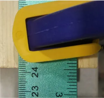
Figure 2.10 With stylus and inkwell connected: original position of the cantilever beam at 0.0212m . . . 16

Figure 2.11 A known weight of 0.077kg is placed underneath the inkwell. The dis-placement observed is 0.0238m . . . 17

Figure 2.12 A steel ball of 0.0952kg is additionally placed on the cantilever beam. The displacement observed is 0.0340m . . . 17

Figure 2.13 Plot of force ’F’ vs displacement ’x’ . . . 18

Figure 2.14 With no stylus attached to the cantilever beam, the displacement ob-served is 0.015m . . . 19

Figure 2.16 Adding another known weight of 0.075kg to the cantilever beam.The

total load on the beam is now 0.152kg . . . 20

Figure 2.17 Placing a steel ball and aluminum disk of 0.0952kg and 0.077kg respec-tively the cantilever beam. The total load on the beam is now 0.1722kg 20 Figure 2.18 Plot of Force ’F’ vs displacement ’x’ for only inkwell placement on the cantilever beam. . . 21

Figure 2.19 With a minimum load from the inkwell, the cantilever beam is placed at 0.017m . . . 22

Figure 2.20 With load of 0.077kg + 0.075kg = 0.152kg placed on top of the inkwell, the cantilever beam is placed at 0.0345m . . . 22

Figure 2.21 For a maximum external load of0.2472kg placed on top of the inkwell, the cantilever beam is placed at 0.0421m . . . 23

Figure 2.22 With the load placed on top of the inkwell the plot for force ’F’ vs displacement ’x’ is observed as above . . . 23

Figure 2.23 For various values of amplitude factor ’a’ the saturation is observed at -4N . . . 25

Figure 2.24 For an input force the spring force exerted by the cantilever beam is observed . . . 25

Figure 2.25 Step response of the Phantom Omni for forces in the range from 1N to 4N . . . 26

Figure 2.26 The transient peak data points used to determine the peak overshoot . 27 Figure 2.27 For a step input with reference to theσ - jω axis, the x-axis represents the attenuation σ=ζωn . . . 28

Figure 3.1 A basic block diagram representing the master-slave system . . . 29

Figure 3.2 Modified block diagram representing the master-slave system . . . 30

Figure 3.3 With no delay and dynamics the master-slave system . . . 32

Figure 3.4 No delay with dynamics: master-slave system . . . 33

Figure 3.6 With delay, dynamics and compensation: master-slave system . . . 35

Figure 4.1 Basic block diagram representing the master-slave system . . . 36

Figure 4.2 With no delay and dynamics the master-slave system . . . 37

Figure 4.3 Root locus of the system with no delay and dynamics . . . 38

Figure 4.4 Step response of the system with no delay and dynamics . . . 38

Figure 4.5 No delay with dynamics: master-slave system . . . 39

Figure 4.6 Root locus of the system with dynamics and no delay . . . 39

Figure 4.7 Step response of the system with dynamics and no delay . . . 40

Figure 4.8 With delay and dynamics: master-slave system . . . 41

Figure 4.9 Root locus of the system with delay and dynamics . . . 41

Figure 4.10 Zoomed Root locus of the system with delay and dynamics depicting master and slave system poles . . . 42

Figure 4.11 Step response of the system with delay and dynamics . . . 42

Figure 4.12 With delay, dynamics and compensation: master-slave system . . . 43

Figure 4.13 Ziegler Nichols tuning method : sustained oscillations for a critical gain valueKu = 122 . . . 43

Figure 4.14 Ziegler Nichols tuning method : Measuring the period of sustained os-cillations asTu= 30sec . . . 44

Figure 4.15 Root locus of PD controller designed using Ziegler Nichols tuning method : Kp = 97.6 and Kd= 366 . . . 45

Figure 4.16 Zoomed Root locus of PD controller designed using Ziegler Nichols tun-ing method : Kp = 97.6 and Kd= 366 . . . 45

Figure 4.17 Step response of PD controller designed using Ziegler Nichols tuning method : Kp = 97.6 andKd= 366 . . . 46

Figure 4.18 Root locus of PD controller designed using manual parameters : Kp = 95 andKd= 410 . . . 46

Figure 4.20 Step response of PD controller designed using manual parameters :

ACKNOWLEDGEMENTS

I would like to express my gratitude to Dr. Greg R. Luecke for his constant support

and encouragement. His insights and enthusiasm guided me through the research and the

writing of this report. I would also like to thank Dr. Ratnesh Kumar for helping me build an

ABSTRACT

Time delay or dead time is defined as the response time required for a process/ a device

when an input is applied. Dead time is a phenomena commonly occurring in industrial

pro-cesses, biological systems and engineering applications. Transport lags, communication lags,

computational delays are various types of time delays which inherently cause improper

func-tioning of the system unless compensated for. Bilateral telemetry is one such application which

faces instability in operation when subjected to time delay. The master robot in the virtual

environment is ’motion and force coupled’ with the slave robot in the virtual environment. This

bilateral feedback provides better tracking results as compared to the unilateral scenario at the

cost of introducing a transport lag in the communication channel. The present work focuses

on addressing this time delay using classical control methods to provide for stability in event

CHAPTER 1. OVERVIEW

Teleoperation is defined as the remote control of machines electronically.The arrangement

consists of a master robot placed in the virtual environment and a slave robot in the actual

environment. The force applied by the operator controls the position of the master robot.

This force acts as a position command for the slave robot. The term ’bilateral’ arises due the

position data of the slave robot fedback to the master robot to enhance the performance of the

teleoperating system.[1] This setup is shown in Figure 1.1.

Figure 1.1: Teleoperation Setup

Teleoperation has been in use in the nuclear industry to safeguard and reduce human

intervention in the field operating areas. The early applications of bilateral feedback used servo

controllers on both master and slave side to reflect the position of the slave to the master as an

input force is applied.[5] For applications in undersea or outer space areas the large distances

between master and slave robots cause a significant delay in the data transmission. This delay

is due to the transmission losses in the communication channels and impacts the stability of

the system. Passivity and scattering theory have been used in the past to address this issue.[1]

in both unilateral[4] and bilateral operations.[7] The variable signal transmission times of the

Internet have been compensated for using event based approach[2] using the non-time based

references on the slave and the sensor.[11] In this work, we propose the use of classical control

methods in discrete domain to address the stability of the system with time delay. We have

used Internet as a communication medium between the master and slave. The communication

delay is assumed to be constant. The architecture used for such an experiment consists of two

CHAPTER 2. MATHEMATICAL MODELING

2.1 Mathematical Model for the Robotic Arm

Consider a simple master-slave system. We propose the use of two ’Phantom Omni’ robots

manufactured by Sensable Devices. Since both the robots are identical there is zero kinematic

mismatch. Hence, we can represent both the haptic arms as electromechanical motor systems

with voltage as the input and position as the output.

Figure 2.1: Schematic of a DC motor [3]

As shown in the figure 2, a DC motor consists of field wound on an iron core named as

stator. The stator is the stationery part of the motor.The iron cylinder placed in between

the poles of the magnet is the rotating part of the motor which constitutes as the rotor. The

rotating coils wound on the rotor known as armature windings. A commutator consisting of

low resistance carbon brushes are connected to the stator which come into contact with the

rotor on application of a current source. When a current is passed through the rotor, the rotor

For the purpose of modeling we interpret the DC motor as follows:

EA

RA

IA LA

−

+

em

LF

RF

EF

τe, ω

J

τA, θA

R1

R2

N τA+θo N τA

Jo

Joω˙o Boω D

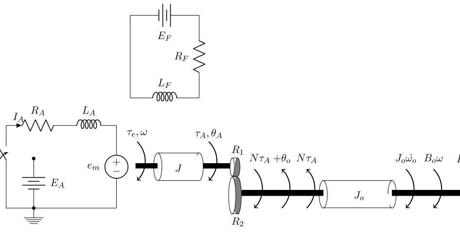
Figure 2.2: Mechanical and Electrical representation of a motor

The armature can be represented as a circuit consisting of armature resistance RA,

in-ductance LA, supply voltage EA and induced voltageem. The magnetic field induced can be

represented as a circuit consisting of field resistance RF, inductance LF and a supply voltage

EF. The back emf observed in the motor is represented asKe.[3]

The rotor has a moment of inertia Jm, damping due to back emf of the motor Bm and a

driving torqueτe which constitute the mechanical equation for motor as follows:

Jms2θm+Bmsθm+τA=τe

The electromechanical torque exerted on the rotor is proportional to the current flowing

through it:

For the gear input/output the equation can be written as:

τA

R2

R1

=N τA

∴ R2

R1

=N

The output inertia is given by:

Jos2θo+Bosθo=N τA+D

Combining the above equations:

Jms2θm+Bmsθm+

Jos2θo+Bosθo−D

N =τe

where

θm=N θo

Jms2θm+Bmsθm+

Jos2θo

N +

Bosθo

N −

D N =τe

(JmN2+Jo)sωo+ (BmN2+Bo)ωo =N τe+D

In terms of output shaft:

Jeqsωo+Beqωo=N τe+D

where :

Jeq=JmN2+Jo

For the electrical circuit representation we can write the Kirchoff’s voltage equation as

follows:

LAi(t) +RAi(t) +Keω=Vin

Laplace transform of the above equation gives:

LAsI+RAI+Keω=Vin

which can be written for the current I as follows:

LAsI=Vin−RAI−Keω

− + Vin − + 1 LA

LAsI 1

s

sI I

RA

Keωm

Reducing the loop:

−

+

Vin 1

RA

1

τEs+ 1

I

Keωm

The mechanical equation for the highest order of ω0 is given by:

Jeqsωo =N τe+D−Beqωo

N Km I + + − + 1 Jeq

Jeqsωo ₁

s

sωo 1

s

ωo θo

Beq

Beqωo

D

Reducing the loop:

N Km

I + + 1 Beq 1 Jeq Beq

s+ 1

1

s ωo

D

θo

Connecting the two blocks we obtain:

−

+

Vin 1

RA

1

τEs+ 1

Keωm

N Km

I + + 1 Beq 1 Jeq Beq

s+ 1

ωo 1

s

θo

D

If we assume no dependence on motor speed and no disturbance ’D’, the block diagram

becomes:

1

RA

Vin 1

τEs+ 1

N Km

I 1

Beq

1

Jeq

Beq

s+ 1

ωo 1

s

θo

Since RA,N Km and Beq are constants, clubbing them together as a constant ’C’:

C = 1

RA

×N Km× 1

Beq

C

Vin 1

τEs+ 1

1

Jeq

Beq

s+ 1

1

s

ωo θo

The effect of motor inductanceτE is negligible and hence can be ignored for this application.

Thus for modeling purposes, the motor equations can be solely represented using the rotor

moment of inertia ’Jeq’ and the damping due to back emf ’Beq’.

C Jeq

Beq

s+ 1

Vin 1

s

ωo θo

Hence, the complete motor block diagram becomes:

−

+

Vin 1

RA

N Km

I +

+ 1

Jeqs+Beq

1

s

ωo θo

D

N

Ke _ω

m

Keωm

For our application, the disturbance ’D’ is in fact operator hand force ’Fhand’. Hence

re-writing the block diagram as follows :

Fhand −

+ 1

Jeqs+Beq

1

s

ωo θo

N2KeKm

RA

Vin

Since, force and voltage are analogous quantities, solving the above block diagram, the

transfer function for the robotic arm with force ’Fhand’ as the input and position ’θo’ as the

output gives :

θo

Fhand

= 1

Jeqs2+Beqs+

N2KmKes

RA

= 1/Beq2

where:

Beq2=Beqs+

N2KmKes

RA

τ = Jeq

2.2 Calculating the Environmental Stiffness

P

Figure 2.3: Spring force experienced by an elastic body when subjected to a load ’P’ [6]

For an elastic body, application of an external force causes deformation which is resisted by

the internal forces. For a spring, such an application of force(load) causes deformation in form

of displacement.

This type of force acting on the spring or any elastic body is called as the ’spring force’

which is given by:

P =Ku

where:

P : spring force

K : spring constant

u : displacement due to forceP

As the force varies, the displacement produced by the spring varies. This relation remains

linear for a small value of the force and as the value of the force increases, the nonlinearity is

apparent(Figure2.4).

The cantilever beam is one such type of elastic body which has been utilized in our

exper-iment to calculate the environmental stiffness. The environmental stiffness can be considered

as an analogous quantity to the spring constant. For our application, environmental stiffness is

defined as the opposition created by the surrounding which the slave robot has to overcome to

follow the desired trajectory as governed by the master robot. The slave system can be

anal-ogously depicted as a mass-spring system. The spring force generated when the slave robot is

placed in the virtual environment is given as follows:

FE =KE×xslave

Using the equation for spring force of the beam the environmental stiffnessKE is given by:

KE = 3EI

L3

where:

L : length of the beam

E : Young’s modulus of elasticity

I : moment of inertia of the beam

For our experiment, we have represented the cantilever beam with a standard 30 cm ≡

0.3m long steel ruler. The ruler is clamped at one end using a wooden support of 0.04m

thickness. The other end of the ruler consists of a fixed Phantom Omni inkwell of measured

weight 0.025kg. The inkwell is used for fixing the stylus position. The weight of the stylus

is known to be 0.020kg [8]. Thus the total fixed load on the cantilever beam(steel ruler) is

0.045kg. When not in operation, this is the maximum load that the cantilever beam will be

subjected to. During the course of the operation, the total load on the beam depends on the

mass of the stylus and the variable mass of the operator’s arm - whether the arm is outstretched

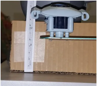
Figure 2.5: Interaction of the Slave robot with the Environment

Because of the fixed position of the inkwell on the ruler as shown in Figure 2.5, the length

of the beam ’L’ is is calculated as follows:

L = clamping position of the ruler - inkwell position

Figure 2.6: Clamping of the steel ruler at 0.247m

To observe a sufficient amount of spring force, the clamping position of the ruler was

chosen at 0.247m(Figure2.6). The inkwell was placed ≈at 0.013m location(Figure 2.7). This

Figure 2.7: Fixing the inkwell on the steel ruler at 0.013m

Thus, the length of the beam ’L’ is:

L= 0.234m

Since the ruler is made of steel, the Young’s modulus of the ruler is observed as:

E= 69−72×109GP a

The steel ruler can be approximated as a rectangular object. Hence, the moment of inertia

’I’ of the cantilever beam can be determined using the standard inertia equation for a rectangle

given by:

I = bh

3

12

where:

b : base or width of the rectangle

Figure 2.8: Measuring the height of the steel ruler

As shown in Figures 2.8 and 2.9, a vernier calliper was used to measure the beam height

and the beam width.The beam height and the beam width were observed to be 0.0015 meters

and 0.03 meters respectively.

This leads to the moment of inertia being calculated as:

I = bh

3

12 =

0.03×(0.0015)3

12 = 8.449×10 −12_m4

While calculating the height of the steel ruler, the following phenomenon was observed:

The etch markings on the steel ruler contributed a significant amount to the measurement of

the height h= 0.0015m. We consider a case where the environmental stiffness KE is assumed

to be 100N/m. Using the values of :

L= 0.234m,E = 69×109GP a,b= 0.03m

we reverse calculate the height of the beam as follows:

h= 3 r

12KL3

3bE

which gives h as:

Figure 2.9: Measuring the width of the steel ruler

This error of one ten-thousandth of an inch is due to the etching material coated on the

steel ruler.

Assuming h= 0.0015m we calculate the environmental stiffness as follows:

KE = 3EI

L3

KE =

3×69×109×8.449×10−12 (0.234)3

which gives the value of environmental stiffness as:

KE ≈136.50N/m

To verify this calculated value, we perform the following experiment:

2.2.1 Case 1 : Stylus + inkwell attached to the cantilever beam

We consider the case where the cantilever beam is subjected to its maximum non operating

load i.e. the inkwell and the stylus are connected. The position at the end of the beam

is measured which is termed as the ’original position’ = 0.015m from the base(Figure 2.10).

Figure 2.10: With stylus and inkwell connected: original position of the cantilever beam at 0.0212m

underneath the inkwell position on the cantilever beam. With each load, the displacement is

measured.

Using the standard spring force equation:

F =Kx

where: F =mg

’m’ : mass of the known weights in kilograms

’g’ : acceleration due to gravity = 9.81m/s2

Plotting a graph of force’F’ vs displacement’x’ we calculate the slope which is in turn our

Figure 2.11: A known weight of 0.077kg is placed underneath the inkwell. The displacement observed is 0.0238m

As shown in Figure 2.11, an aluminum disk of known weight 0.077g causes a displacement

of 0.0238m. The actual displacement is calculated as:

Actual displacement = original position - position due to weights

Thus, the actual displacement observed for a mass of 0.077kg is 0.0026m.

Figure 2.12: A steel ball of 0.0952kg is additionally placed on the cantilever beam. The displacement observed is 0.0340m

As shown in Figure 2.12, with the steel ball placed alongwith the aluminum disk the total

Using these data points i.e. displacement with no load, displacement with 0.077kg load and

displacement with 0.1722kg load we plot the graph of force ’F’ vs displacement ’x’ as shown

in Figure 2.13:

Figure 2.13: Plot of force ’F’ vs displacement ’x’

The slope of the line is calculated using the data tips shown in the plot(Figure2.13).

KE =

(1.688−0.7547) (0.0128−0.0026)

2.2.2 Case 2: Inkwell attached to the cantilever beam without the Omni stylus

Figure 2.14: With no stylus attached to the cantilever beam, the displacement observed is 0.015m

We now consider a case where the stylus is disconnected from the cantilever beam. In such

a case the minimum mass subjected to the cantilever beam is that of the inkwell(0.025g). The

original position for such an arrangement is 0.015m as shown in Figure 2.14.

Now, adding a weight of 0.077kg to the cantilever beam causes a displacement of 0.0288.

The actual displacement is thus 0.0288 - 0.015 = 0.0138m(Figure 2.15).

Figure 2.15: Adding a known weight of 0.077kg to the cantilever beam.The beam is now positioned at 0.0288m

Further addition of 75g to the cantilever beam causes the beam location to shift to 0.0308m

Figure 2.16: Adding another known weight of 0.075kg to the cantilever beam.The total load on the beam is now 0.152kg

Figure 2.17: Placing a steel ball and aluminum disk of 0.0952kg and 0.077kg respectively the cantilever beam. The total load on the beam is now 0.1722kg

For a steel ball and an aluminum disk placed on the cantilever beam, the displacement

Using these data points, the plot of force ’F’ vs displacement ’x’ is given by:

Figure 2.18: Plot of Force ’F’ vs displacement ’x’ for only inkwell placement on the cantilever beam.

The data is curve fitted(shown by a red line) to estimate the environmental stiffness as

follows:

KE =

(1.586−1.004) (0.01995−0.01285)

2.2.3 Case 3: Inkwell attached to the cantilever beam with the weights placed on top of the inkwell

We now consider the case where only the inkwell is connected to the cantilever beam and

the weights are placed on top of the inkwell.

Figure 2.19: With a minimum load from the inkwell, the cantilever beam is placed at 0.017m

With no weight attached to the cantilever beam, the only load is that of the inkwell with

measured weight 0.025kg. As shown in Figure2.19 the original position recorded is 0.017m.

Now by placing two aluminum disks of 0.077kg and 0.075kg on top of the inkwell, the total

load to which the cantilever beam is subjected is 0.152kg. The actual displacement observed

is 0.0175m. This is shown in Figure 2.20.

Figure 2.21: For a maximum external load of0.2472kg placed on top of the inkwell, the cantilever beam is placed at 0.0421m

As shown in Figure2.21or a total external load of 0.0952kg(steel ball) + 0.077kg(aluminum

disk 1) + 0.075kg(aluminum disk 2) = 0.2472kg, the actual displacement recorded is 0.0251m.

Using this data, the graph of force ’F’ vs displacement ’x’ is plotted as follows:

Figure 2.22: With the load placed on top of the inkwell the plot for force ’F’ vs displacement ’x’ is observed as above

The environmental stiffness is thus calculated as:

KE =

(2.423−1.49) (0.0251−0.0175)

From the above three experiments we observe the environmental stiffness value to be

91.5N/m, 82N/m and 122.76N/m respectively. Accounting for frictional forces and round off

errors we can approximate the environmental stiffness value as an average of the three values

obtained experimentally.

Averaging these values thus yields KE = 98.7N/m which for all practical purposes is

approximated as KE = 100N/m.

Further, to observe the relation between ’force’ and ’displacement’, we consider a one

di-mensional application of the Phantom Omni. We send out a force in negative ’y’ direction to

observe the displacement along the y-axis. With no damping i.e. ζ = 0 the force inputted is a

sinusoidal waveform given by:

Fy =a(1−cos(ωt))

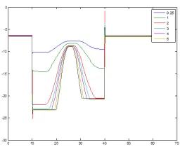
For ω = 0.25 and ω = 0.5, we vary the value of the amplitude factor’a’ from 0.5 to 5.0 in

steps of 0.5. This results in the force valueFy in the range of -1N to -10N.

a Fy(N) Displacementy(m)

0.5 –0.99993 -9.73909 1.0 -2 -14.0298 1.5 -2.99963 -17.7762 2.0 -3.99955 -20.3996 2.5 -4.99997 -20.1961 3.0 -5.99926 -19.948 3.5 -6.99048 -19.7449 4.0 -7.99967 -19.5419 4.5 -8.99969 -19.3392 5.0 -9.99985 -19.6352

Figure 2.23: For various values of amplitude factor ’a’ the saturation is observed at -4N

For Fy = -1 to -4N, the relation between displacement in y-direction and Fy is linear.

For a force beyond -4N, there is saturation in the spring force and hence the nonlinearity is

apparent(Figure2.23).

Figure 2.24: For an input force the spring force exerted by the cantilever beam is observed

As can be seen from the Figure 2.24 there is a decrease in the amplitude of the sine wave

observed at the output of the Phantom Omni. This decrease in the amplitude is due to the

2.3 Calculating the natural frequency and damping ratio

Figure 2.25: Step response of the Phantom Omni for forces in the range from 1N to 4N

For the one dimensional application of the Phantom Omni, a force in the negative

y-direction ranging from 1N to 4N was inputted to observe the displacement in y-y-direction. This

force was inputted as a step force decreasing in magnitude with every 10 seconds(Figure2.25).

This resulted in a scenario where the Phantom Omni was subjected to disturbances of varied

amplitudes. For every transition, the response of the Omni was observed. This was useful in

determining the transient characteristics of the system.

The main operational device inside the Phantom Omni is a DC motor. Using section 2.1

we can say that the equation governing the robotic arm is a standard second order system.

This allows us to use the standard transient response characteristics associated with a second

order system. The peak overshoot for the system was calculated using the reading in green

Figure 2.26: The transient peak data points used to determine the peak overshoot

Using the data points in Figure 2.26we calculate the peak overshoot ’Mp’ as follows:

Mp =

(−7.507−(−6.324)) (−7.507)

Mp = 0.1575

Using the standard formula:

Mp = exp−ζπ/ √

1−ζ2

×100

the damping ratio was calculated as:

Figure 2.27: For a step input with reference to the σ - jω axis, the x-axis represents the attenuation σ=ζωn

The displacement along the x-axis which is equivalent toζωnor the attenuation was found

out to be 0.3.

ζωn= 0.3

∴ωn= 0.3

ζ = 0.3333rad/sec

Using these values of ωn = 0.3333rad/sec, ζ = 0.9 and KE = 100N/m we have designed

the second order representation for the Phantom Omni.

Since, two Phantom Omnis are utilized to represent the master and slave systems

respec-tively; their architectures are same i.e. they are represented using the same second order

CHAPTER 3. CONTROL SYSTEM DESIGN

With the experimentally calculated values of damping ratio ’ζ’, natural frequency ’ωn’ and

environmental stiffness ’KE’ we now construct a block diagram structure to observe the effects

of various dynamics introduced by the mathematical modeling.

−

+

Fhand C

τ s+ 1

Master system

Fnet 1

s

˙

xmaster

∆T

xmaster 1

KE

ω_n2 s2_{+ 2ζω}

ns+ωn2

Slave system xslave KE ∆T Fslave RA

KmN

Control Gain

KmN

RA Vin

Fmaster

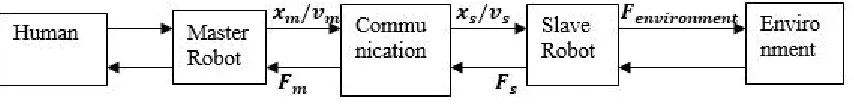
Figure 3.1: A basic block diagram representing the master-slave system

Figure3.1shows the basic model of a LTI SISO system with force as the input variable and

position as the output variable.The operator in the virtual environment controls the motion

of the master robot. Hence, the input to the system is the hand force commanded by the

operator. The hand force is variable in nature depending on whether the handle is held firmly

or lightly, whether the arm is bent or outstretched.

The actions performed by the master robot are conveyed using a communication

chan-nel(represented as ∆T) to the slave robot. The slave robot in the actual environment

expe-riences certain oppositions. These oppositions as mentioned in section 2.2 are primarily the

The slave robot tries to imitate the actions of the master robot in the actual environment.

This slave imitation data is fedback to the master robot via a communication channel. The data

contains the current position of the slave robot which is incorporated with the environmental

stiffness ’KE’. Thus, the spring force experienced by the slave robot in the environment forms

the feedback loop.

This feedback spring force is applied to the master robot in terms of voltage. This conversion

of force to voltage is done using a control gain of the form:

Control Gain = RA

KmN

The architecture of the Phantom Omni is such that it allows for an internal adjustment of

voltage to force conversion. Hence, it is no longer impertinent to represent the control gain

and the conversion factor from voltage to force.

Compensating the force to voltage conversion blocks we can form the block diagram as

follows:

−

+

Fhand C

τ s+ 1

Fnet 1

s

˙

xmaster

Master system

∆T

xmaster 1

KE

ω_n2 s2_{+ 2ζω}

ns+ωn2 Slave system xslave KE ∆T Fslave Fmaster

Figure 3.2: Modified block diagram representing the master-slave system

The force from the master robot is sent to the slave robot using a communication channel

and vice versa. The communication channel proposed is User Datagram Protocol(UDP). It

is observed that the communication channel creates a delay in the transmission of data from

master robot to the slave robot and vice versa. This communication delay significantly impacts

For the slave system, the standard second order equation has been used as follows:

ω_n2 s2_{+ 2ζω}

ns+ωn2

If we represent our slave system as a mass spring damper system, the second order equation

becomes:

1

M s2_+Bs+K

E

Thus, the above equations are equivalent and hence we can express mass ’M’, damping ’B’

as follows :

M = KE

ω2

n

B = 2×ζ×ωn×M

In regards to the time constant form used to represent the master system this can be

equivalently written as:

τ = M

B

C= 1

3.0.1 Case 1 : No delay and no dynamics

−

+

Fhand C

τ s+ 1

1 s ˙ x x KE FE

Figure 3.3: With no delay and dynamics the master-slave system

We first consider the ideal case where the system experiences no instability. This consists

of the master system and an accurate execution of the operator’s commands in the actual

environment. The system equation thus becomes:

x Fhand

= C

τ s2_+s+CK

E

At steady state the transfer function becomes:

x Fhand(s=0)

= 1

KE

which shows that the system behavior solely depends on the environmental stiffness and

it’s effects on the manipulator behavior. Any instability due to the environment will affect the

stability of the system. It also shows that any amount of operator’s force will include a factor

of the environmental stiffness. For e.g. if we command the Phantom Omni to travel for 1m

withKE = 100N/m the actual travel will be 0.01m.

3.0.2 Case 2 : No delay with dynamics

We now introduce the dynamics caused by the environment and its association with the

slave system. Using the experimental data from section 2.2 we have determined the values

for damping ratio ζ = 0.9, natural frequency ωn = 0.3333 rad/sec and environmental stiffness

Since the environmental stiffness is observed to be varying the damping ratio ζ and natural

frequencyωn add dynamics which can destabilize the system. This is shown in Figure4.6.

−

+

Fhand C

τ s+ 1

1

s

˙

xmaster 1

KE

xmaster ω_n2

s2_{+ 2ζω}

ns+ωn2

xslave

KE

FE

Figure 3.4: No delay with dynamics: master-slave system

The transfer function for such a system becomes:

xslave

Fhand

= Cω

2

n (τ s2_+s)(s2_{+ 2ζω}

ns+ωn2) + (Cωn2KE) For the steady state condition the transfer function becomes:

xslave

Fhand(s=0)

= 1

KE

This shows that the stability of the system depends on dynamic nature of the environment

of operation.

3.0.3 Case 3 : With delay and dynamics

The delay included in the block diagram is shown as ’∆T’. However, in actual calculations

the delay is represented as ’e−sT_{’. To express this delay of ’e}−sT_{’ mathematically we use Pade}

approximation to represent the Taylor series with an approximate value. In the present work,

we have used the first order Pade approximation to represent the time delay as :

e−sT = −s+a

s+a

Since the time delay model introduces a zero in the right half s-plane, the system is subjected

Figure 4.9.

−

+

Fhand C

τ s+ 1

1

s

˙

xmaster −s+a

s+a

xmaster 1

KE

ω2_n s2_{+ 2ζω}

ns+ωn2

xslave

KE −s+a

s+a FE

Figure 3.5: With delay and dynamics: master-slave system

The system transfer function for such a system is calculated to be as follows:

xslave

Fhand

= Cω

2

n(−s+a)(s+a) (τ s+ 1)(s)(s+a)(s2_{+ 2ζω}

ns+ωn2)(s+a) +CKE(−s+a)2ωn2 At steady state :

xslave

Fhand(s=0)

= 1

KE

Thus it can be seen that the effects of the non-minimum phase contribute to the transient

effect of the system. The steady state solely depends on the effects of the environment in which

3.0.4 Case 4: With delay, dynamics and compensation

−

+

Fhand C

τ s+ 1

1

s

˙

xmaster −s+a

s+a

xmaster 1

KE

ω2_n s2_{+ 2ζω}

ns+ωn2

xslave

KE −s+a

s+a Kp(s+ac)

FE

Figure 3.6: With delay, dynamics and compensation: master-slave system

To compensate for the varying nature of the environmental stiffness and the time delays,

we introduce a PD controller. The controller is designed in association with the slave system

and hence the slave system can be modeled as a position input and position output system.

The PD controller is able to stabilize the system although unstable poles are observed.

The transfer function thus becomes:

xslave

Fhand

= Cω

2

n(−s+a)(s+a) (τ s+ 1)(s)(s+a)2_(s2_{+ 2ζω}

ns+ω2n) +CKEωn2(−s+a)2(Kp(s+ac))

At steady state :

xslave

Fhand(s=0)

= 1

KpacKE

Thus the proportional gain and the derivative gain act as a compensation for any instabilities

CHAPTER 4. RESULTS

With reference to the design scenarios discussed in chapter 3, we now use MATLAB to

simulate the results for the closed loop system response.

−

+

Fhand C

τ s+ 1

Fnet 1

s

˙

xmaster

∆T

xmaster 1

KE

ω_n2 s2_{+ 2ζω}

ns+ωn2

xslave

KE ∆T

Fslave

Fmaster

Figure 4.1: Basic block diagram representing the master-slave system

With damping ratio ζ = 0.9, natural frequency ωn = 0.3333rad/sec and environmental

stiffness KE = 100N/m, the values of ’C’,’τ’,’M’ and ’B’ are computed as follows:

M = KE

ω2

n

M = 900kg

B = 2×ζ×ωn×M

τ = M

B

τ = 1.6667sec

C= 1

B

C = 0.0019m/N s

Using these values, we compute the transfer functions for each of the cases mentioned in

chapter 3. The root locus technique has been utilized to observe the behavior of the closed

loop system and the impact of delay on such systems. The step response is used to analyze the

accuracy of our design in the event of disturbances due to varying nature of the environment

or the delays in communication channel.

All the results tested so far are for a time delay ofT = 0.0001seconds

4.0.1 Case 1 : No delay, no dynamics

−

+

Fhand C

τ s+ 1

1

s

˙

x x

KE

FE

Figure 4.2: With no delay and dynamics the master-slave system

x Fhand

= 0.001852 1.667s2_{+s+ 0.1852}

Figure 4.3: Root locus of the system with no delay and dynamics

The root locus shows a pair of complex conjugate poles in the left half s-plane indicating

that the system is stable.

For a step input the response is recorded as follows:

Figure 4.4: Step response of the system with no delay and dynamics

The step response indicates that the system stabilizes within a settling time of 14.1 seconds

since no delay or dynamics interfere with it’s stability.

This shows that for any given input from the master robot, the slave robot will take 14.1

4.0.2 Case 2: No delay, with dynamics

−

+

Fhand C

τ s+ 1

1

s

˙

xmaster 1

KE

xmaster ω_n2

s2_{+ 2ζω}

ns+ωn2

xslave

KE

FE

Figure 4.5: No delay with dynamics: master-slave system

xslave

Fhand

= 2.058×10 −6

1.667s4_{+ 2s}3_{+ 0.7852s}2_{+ 0.1111s+ 0.0002058}

With the dynamics of the slave + environment system added to the closed loop transfer

function, the root locus now becomes:

Figure 4.6: Root locus of the system with dynamics and no delay

The two complex conjugate poles are due to the slave system while the two single poles :

one at the origin and the other at 1

τ belong to the master system. The pole at the origin and

one of the complex conjugate poles converge to the right half of the s-plane thus marking that

Figure 4.7: Step response of the system with dynamics and no delay

Due to the pole at the origin and the complex pole converging in the right half s-plane the

system takes longer time to stabilize (Settling time = 2.09×103 seconds). This response to a

4.0.3 Case 3: With delay and dynamics

−

+

Fhand C

τ s+ 1

1

s

˙

xmaster −s+a

s+a

xmaster 1

KE

ω2_n s2_{+ 2ζω}

ns+ωn2

xslave

KE −s+a

s+a FE

Figure 4.8: With delay and dynamics: master-slave system

With delay introduced into the system as a Pade approximation of 1st order, we now

compute the transfer function of the system as follows:

xslave

Fhand

= −2.058×10

−6_s2_{+ 823}

1.667s6_{+ 6.667×10}4_s5_{+ 6.667×10}8_s4_{+ 8×10}8_s3_{+ 3.141×10}8_s2_{+ 4.444×10}7_{s+ 8.23×10}4

This block diagram shows that there is a proportional gain Kp= 1 present in the system.

The root locus for such a system was observed to be as follows:

Figure 4.10: Zoomed Root locus of the system with delay and dynamics depicting master and slave system poles

Due to the Pade approximation, there is an introduction of zero in the right half s-plane.

The pole of the Pade approximation is canceled by another zero created during the formulation

of the transfer function.

Figure 4.11: Step response of the system with delay and dynamics

For a system with time delay, the system settles at 1.17×103 seconds. This settling time

is less than the one observed in section 4.0.2. It is because the dominant roots belong to the

Pade approximated time delay system and the slave dynamics due to environment have very

4.0.4 Case 4: With delay, dynamics and compensation

−

+

Fhand C

τ s+ 1

1

s

˙

xmaster −s+a

s+a

xmaster 1

KE

ω2_n s2_{+ 2ζω}

ns+ωn2

xslave

KE −s+a

s+a Kp(s+ac)

FE

Figure 4.12: With delay, dynamics and compensation: master-slave system

To tune the PD controller, Ziegler-Nichols method was used. The integral gainKI and the

derivative gain Kd were made zero. The proportional gain Kp was increased to a value such

that sustained oscillations were observed.[9]

Figure 4.13: Ziegler Nichols tuning method : sustained oscillations for a critical gain value

Ku = 122

The sustained oscillations were observed for Kp = 122. This is the critical gain ’Ku’. The

period of oscillation for this critical gain is ’Tu = 30sec’. This is shown in Figures 4.13 and

4.14.

Figure 4.14: Ziegler Nichols tuning method : Measuring the period of sustained oscillations as

Tu= 30sec

Kp = 0.8Ku= 97.6

Td=

Tu

8 = 3.75

the PD controller equation becomes :

C(s) =Kp(1 +Tds)

C(s) = 97.6(1 + 3.75s)

C(s) = 97.6 + 366s

which becomes:

xslave

Fhand

= −2.058×10

−6_s2_{+ 823}

1.667s6_{+ 6.667×10}4_s5_{+ 6.667×10}8_s4_{+ 8×10}8_s3_{+ 3.141×10}8_s2_{+ 7.457×10}7_{s+ 8.033×10}6

Using this controller, the root locus becomes :

Figure 4.15: Root locus of PD controller designed using Ziegler Nichols tuning method : Kp = 97.6 andKd= 366

Figure 4.17: Step response of PD controller designed using Ziegler Nichols tuning method :

Kp = 97.6 andKd= 366

The step response is observed in Figure4.17. This shows that even though there are unstable

poles and zeros in the transfer function of the master-slave system, the PD controller is able

to compensate for these instabilities and provide for a settling time of 24.9 seconds.

Further using some manual computation, theKp value was adjusted to 95 and theKdvalue

was changed to 410. This yielded a system with better settling time.

Figure 4.18: Root locus of PD controller designed using manual parameters : Kp = 95 and

Figure 4.19: Zoomed Root locus of PD controller designed using manual parameters : Kp= 95 and Kd= 410

The settling time of this system was observed to be 17.3 seconds which is better compared

to that obtained using the Ziegler-Nichols tuning method(Figure 4.20).

Figure 4.20: Step response of PD controller designed using manual parameters : Kp = 95 and

CHAPTER 5. CONCLUSION

In this report we introduce the concept of time delay and it’s implications to various fields

of applications requiring human safety and intervention. We introduced the Phantom Omni

haptic devices as the hardware to design the system identification parameters: damping ratio

’ζ’ and natural frequency of oscillation ’ωn’. We further use the Phantom Omni haptic device

to determine the environmental stiffness value. This forms our system identification process.

Using these parameters has helped us in simplifying the mathematical model for our

master-slave system. Developing the master and slave systems as standard second order systems

has allowed us to use the standard transient response characteristics to the study the system

behavior.

To simplify the analysis, we propose the use of classical control methods to determine the

system stability regions. Using the root locus technique helps us in building an intuition of the

system behavior in event of large time delays. As can be seen, a proportional plus derivative

(PD) controller can provide for a sufficient control during time delayed operation. To enhance

the design further, a lead compensator can be designed to accurately design the location of the

Specifications for the PHANTOM Omni® haptic device

Corporate Headquarters

SensAble Technologies, Inc. 15 Constitution Way Woburn, MA 01801 USA [t] +1-781-937-8315 [f] +1-781-937-8325 email: [email protected] Web: www.sensable.com

© 1993-2008 SensAble Technologies, Inc. All rights reserved. OpenHaptics, PHANTOM, PHANTOM Desktop, PHANTOM Omni, SensAble, and SensAble Technologies, Inc. are trademarks or registered trademarks of SensAble Technologies, Inc. Other brand and product names are trademarks of their respective holders. Product specifications are subject to change without notice. The SensAble Technologies PHANTOM® product line of haptic devices makes it possible for users to touch and manipulate virtual objects. Different PHANTOM devices meet varying needs. The Premium models are high-precision instruments and, within the PHANTOM product line, provide the largest workspaces and highest forces, and some offer 6DOF (6 degrees of freedom) output capabilities. The PHANTOM Omni model is the most cost-effective haptic device available today. Portable design, compact footprint, and IEEE-1394a FireWire® port interface ensure quick installation and ease-of-use.

Model The PHANTOM Omni Device

Force feedback workspace ~6.4 W x 4.8 H x 2.8 D in > 160 W x 120 H x 70 D mm Footprint

Physical area the base of device occupies on the desk

6 5/8 W x 8 D in ~168 W x 203 D mm Weight (device only) 3 lb 15 oz

Range of motion Hand movement pivoting at wrist

Nominal position resolution

> 450 dpi ~ 0.055 mm Backdrive friction <1 oz (0.26 N) Maximum exertable force at nominal

(orthogonal arms) position 0.75 lbf. (3.3 N) Continuous exertable force (24 hrs.) > 0.2 lbf. (0.88 N)

Stiffness

X axis > 7.3 lb/in (1.26 N/mm) Y axis > 13.4 lb/in (2.31 N/mm)

Z axis > 5.9 lb/in (1.02 N/mm) Inertia (apparent mass at tip) ~0.101 lbm. (45 g)

Force feedback x, y, z Position sensing

[Stylus gimbal]

x, y, z (digital encoders)

[Pitch, roll, yaw (± 5% linearity potentiometers)] Interface IEEE-1394 FireWire® port:

6-pin to 6-pin* Supported platforms Intel or AMD-based PCs OpenHaptics® SDK compatibility Yes

Bibliography

[1] Anderson, R. J. and Spong, M. W. (1989). Bilateral control of teleoperators with time

delay. IEEE Transactions on Automatic Control, 34(5):494–501.

[2] Brady, K. and Tarn, T. J. (2001). Internet-based teleoperation. InProceedings 2001 ICRA.

IEEE International Conference on Robotics and Automation (Cat. No.01CH37164),

vol-ume 1, pages 644–649 vol.1.

[3] Close, C. M., Frederick, D. K., and Newell, J. C. (2002). Modeling and analysis of dynamic

systems; 3rd ed. Wiley, New York, NY.

[4] Coristine, M. and Stein, M. R. (2004). Design of a new pumapaint interface and its use

in one year of operation. In Robotics and Automation, 2004. Proceedings. ICRA ’04. 2004

IEEE International Conference on, volume 1, pages 511–516 Vol.1.

[5] GOERTZ, R. C. (1964). Manipulator systems developed at anl. Proceedings, The 12th

Conference on Remote Systems Technology, pages 117–136.

[6] Humar, J. L. (1990). Dynamic of Structures. Prentice-Hall, Inc., Upper Saddle River, NJ,

USA.

[7] Munir, S. and Book, W. J. (2002). Internet-based teleoperation using wave variables with

prediction. IEEE/ASME Transactions on Mechatronics, 7(2):124–133.

[8] Najdovski, Z. and Nahavandi, S. (2008). Extending haptic device capability for 3d virtual

grasping. In Ferre, M., editor, Haptics: Perception, Devices and Scenarios, pages 494–503,

Berlin, Heidelberg. Springer Berlin Heidelberg.

[10] Wikipedia contributors (2004). Zieglernichols method — Wikipedia, the free encyclopedia.

[Online; accessed 22-July-2004].

[11] Xi, N. and Tarn, T. J. (1999). Action synchronization and control of internet based

telerobotic systems. In Proceedings 1999 IEEE International Conference on Robotics and