www.ann-geophys.net/24/2043/2006/ © European Geosciences Union 2006
Annales
Geophysicae
Interchange instability of the plasma disk in Jupiter’s middle
magnetosphere and its relation to the radial plasma density
distribution
P. A. Bespalov1, S. S. Davydenko1, S. W. H. Cowley2, and J. D. Nichols2
1Institute of Applied Physics, Russian Academy of Sciences, 46 Ulyanov St, 603950 Nizhny Novgorod, Russia 2Department of Physics & Astronomy, University of Leicester, Leicester LE1 7RH, UK
Received: 24 November 2005 – Revised: 19 April 2006 – Accepted: 23 June 2006 – Published: 9 August 2006
Abstract. We analyse the interchange or flute instability
of the equatorial plasma disk in Jupiter’s middle magneto-sphere. Particular attention is paid to wave coupling between the dense plasma in the equatorial disk and the more rarefied plasma at higher latitudes, and between the latter plasma and the conducting ionosphere at the feet of the field lines. It is assumed that the flute perturbations are of small spatial scale in the azimuthal direction, such that a local Cartesian approx-imation may be employed, in which the effect of the cen-trifugal acceleration associated with plasma rotation is rep-resented by an “external” force in the “radial” direction, per-pendicular to the plasma flow. For such small-scale perturba-tions the ionosphere can also be treated as a perfect electri-cal conductor, and the condition is determined under which this approximation holds. We then examine the condition under which flute perturbations are at the threshold of insta-bility, and use this to determine the corresponding limiting radial density gradient within the plasma disk. We find that when the density of the high-latitude plasma is sufficiently low compared with that of the disk, such that coupling to the ionosphere is not important, the limiting radial density profile within the disk follows that of the equatorial mag-netic field strength as expected. However, as the density of the high-latitude plasma increases toward that of the equato-rial disk, the limiting density profile in the disk falls increas-ingly steeply compared with that of the magnetic field, due to the increased stabilising effect of the ionospheric interac-tion. An initial examination of Galileo plasma density and magnetic field profiles, specifically for orbit G08, indicates that the latter effect is indeed operative inside radial distances of∼20RJ. At larger distances, however, additional density smoothing effects appear to be important.
Keywords. Magnetospheric physics (Magnetospheric
con-figuration and dynamics; MHD waves and instabilities; Plan-etary magnetospheres)
Correspondence to: P. A. Bespalov
1 Introduction
Region II
Region I
z l=
z d=
z d
=-z l =-g
B z
x
Ionosphere
Ionosphere
[image:2.595.64.269.61.264.2]B y
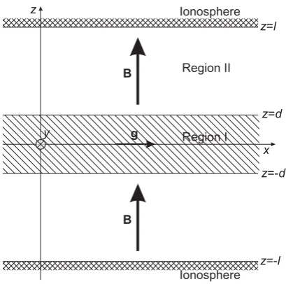
Fig. 1. Sketch of the local Cartesian system analysed in this pa-per. A slab of high-density iogenic plasma (shown hatched), termed “region I”, lies in thex−y plane in the region given by |z| ≤d, thus centred on the equatorial plane atz=0. Outside the slab lies a more tenuous plasma on either side, termed “region II”, which is bounded by the conducting planetary ionosphere atz=±l. The field lines indicated by theBvector are straight, and pass orthogo-nally through the equatorial plasma slab between the ionospheres as shown. The unperturbed field and plasma parameters (such as the field strength, field line length, and plasma density) vary only in the xdirection, thus representing radial distance from the centre of the planet. The unperturbed plasma convective velocity is then in they direction (into the plane of the diagram as shown), representing par-tial plasma corotation with respect to the planetary angular velocity. The acceleration of the disk plasma due to the centrifugal effect of plasma rotation and to field line curvature is then represented by an “external” forcegin thexdirection, as also shown.
The outward-flowing mass-loaded flux tubes are replaced in the interchange process by “unloaded” flux tubes from the outer regions, which contain a tenuous plasma which is compressed and heated during its inward transport. The co-existing plasma populations to which this process gives rise in the jovian middle magnetosphere thus consist of two components. The first is cool dense iogenic plasma, with energies typically below, say,∼10 keV, which diffuses out-wards, mainly confined to near the equatorial plane by cen-trifugal action (e.g. Belcher, 1983; Bagenal, 1994; Frank and Paterson, 2001, 2004). The density of this cool equatorial plasma is observed to fall, at radial distances between∼10 and∼50RJ, approximately as a power law of the distance, with an exponent of∼4–5 (e.g. Gurnett et al., 1981; Divine and Garrett, 1983). The second is a hot tenuous plasma more broadly distributed along the field lines, with energies above ∼10 keV, reaching to 100 s keV in the torus region, which diffuses inward (e.g. Krimigis and Roelof, 1983; Mauk et al., 1996; Woch et al., 2004). The centrifugal action of the
cool component, which contains most of the plasma mass, combined with the pressure gradient of the hot component, which contains most of the plasma thermal energy, then act to stretch the magnetic field lines outward away from the planet, associated with an azimuthal current, which is a character-istic feature of the middle magnetosphere region (Acu˜na et al., 1983; Mauk et al., 1985; Caudal, 1986; Bunce and Cow-ley, 2001; Khurana, 2001).
Although this general picture of the physics of Jupiter’s middle magnetosphere has been current for a significant pe-riod, a detailed understanding of the nature of the associated transport processes, and their relation to the plasma proper-ties, has proven elusive. Initial discussions were based on interchange motions of whole flux tubes, using either as-sumed or observed distributions of field and plasma (e.g. Gold, 1959; Melrose, 1967; Hill, 1976; Goertz, 1980; Hill et al., 1981; Summers and Siscoe, 1985; Pontius et al., 1986; Southwood and Kivelson, 1987; Pontius and Hill, 1989; Huang and Hill, 1991). The results of related computer sim-ulations have also been presented (Yang et al., 1994; Pontius et al., 1998). More recently, the effect of magnetic perturba-tions on the interchange or “flute” instability have been dis-cussed by Liu (1998), while Ferri`ere and Andr´e (2003) have discussed a mixed fluid-kinetic approach to low-frequency instabilities.
In this paper we consider the flute instability in a plasma model in which most of the plasma mass is confined near the equatorial plane, as assumed in many of the works cited above for reasons already discussed, but where tenu-ous plasma is also present outside of the equatorial disk, and account is taken of the communication with the conducting ionosphere at the feet of the field lines. The results of linear stability analysis are used to estimate the equilibrium radial profile of the equatorial plasma, assuming that the growth rate of the most unstable mode is just zero on each field line (e.g. Bespalov and Zheleznyakov, 1990). This estimate pro-vides the steepest radial profile of the plasma density that is stable to the flute modes. This threshold profile can then be further smoothed by slower instabilities, though this aspect is not considered here.
2 Background plasma model and basic equations
For mathematical convenience we consider electrostatic per-turbations in the plasma system with the simplified Cartesian geometry shown in Fig. 1. The cool dense iogenic equatorial plasma (region I) lies in a slab in thex−yplane of thickness 2d, centred onz=0. For simplicity of calculation the plasma in this region is taken to consist of one singly-charged ion species, oxygen in numerical estimates, and electrons, and we also ignore the plasma pressure as discussed further be-low. The magnetic field lines are taken to be straight in the
finite height-integrated Pedersen conductivity6P. The field strengthB and the unperturbed plasma density n(I0) within the slab vary only in thexdirection, which thus represents ra-dial distance from the planet. The unperturbed density of the more rarefied plasma outside the equatorial slab (region II) also varies only withx, and is taken to be a fixed fraction of the slab density, so that
n(I I0)(x)=τ n(I0)(x) , (1) whereτ is a constant less than unity. The unperturbed ro-tational motion of the plasma is then represented as a ve-locity in they direction that depends only onx. Here we take this velocity to correspond to essentially rigid coro-tation of the plasma with the planet out to a distance of 15RJ, at angular velocityJ (equal to 1.76×10⁻⁴rad s−1), after which the velocity remains constant at the value
V=15JRJ≈190 km s−1such that the effective angular ve-locity falls inversely with the distance. This behaviour is based on the velocity measurements obtained from Voy-ager plasma data by Belcher (1983) and Sands and Mc-Nutt (1988). The unperturbed convection velocity is hence given by
Vy=
Jx x ≤15RJ
V =15JRJ x ≥15RJ
. (2)
The centrifugal acceleration associated with this motion in the real rotational system is then represented by an “external” force per unit mass in thexdirection given by
gcfx = Vy2
x , (3a)
which is thus the same for ions and electrons, and for
x≥15RJ (the main region of interest here) is gcfx =
(15JRJ)2
x ≈500
RJ x m s
−2. (3b) For simplicity, this force is ignored for the more tenuous plasma lying outside the slab, an approximation that is ap-propriate for two reasons. The first is that in the real middle magnetosphere current sheet field geometry the centrifugal force per unit mass transverse to the magnetic field will ac-tually fall significantly with distance from the current sheet along a given field line (in thezdirection in our slab model). This is due both to the change in the magnetic field direction relative to the radial vector from the rotation axis, and to the reduction in plasma rotation speed at fixed angular velocity at smaller radial distances from the planet. For simplicity we have thus effectively employed a zero approximation imme-diately outside of the current sheet. The second is that in the jovian middle magnetosphere, typically only a few percent of the total mass of plasma on a given field line lies outside of the current sheet slab. Consequently, the development of the instability will be dominated by the centrifugal effect of
the latter plasma population, as included in our calculation, and the contribution of the plasma mass at higher latitudes will be small.
We also note that despite the fact that the field lines in our simplified model are straight, the effect of the actual curva-ture of the field within the current sheet can also be incor-porated in the model by the inclusion of a second “external” force in thex direction on the plasma in the equatorial slab. Assuming that particle guiding-centre motion is valid within the current sheet, the force per unit mass for particle species
αis
gcurαx = v 2 T α Rc
≈ Tα
mαRc
, (4a)
where Rc is the radius of curvature of the field lines, and mα is the mass of speciesα, whose thermal speed isvT α at temperature Tα. Taking the radius of curvature within the middle magnetosphere current sheet to be∼2RJ (e.g. Mauk and Krimigis, 1987; Staines et al., 1996), and the ion and electron temperatures to be∼100 eV (e.g. Acu˜na et al., 1983; Belcher, 1983), then yields
gcurix ≈ me
mi
gexcur≈ T 2miRJ
∼ 4 m s−2, (4b)
where for definiteness we have taken the ion mass to corre-spond to oxygen. We note that particle guiding-centre mo-tion is indeed valid for these parameters, since even for oxy-gen ions we typically find ρi
RJ
≈10−2within the rele-vant region of the current sheet, whereρi is the ion gyrora-dius, compared with current sheet scales of∼RJ or larger. It can thus be seen that for ions the curvature effect is generally small compared with the centrifugal force, and vice-versa for electrons.
We should comment at this point that the above develop-ment of the problem using straight field lines in a Cartesian geometry forms an approximation that significantly simpli-fies the algebra of the problem and allows a simple treatment of the physical effects of interest. Although this geometry may initially seem a rather poor representation of the jovian middle magnetosphere, we emphasise that the essential fea-tures of the “current sheet” form of the field lines are in fact appropriately included via the “external” forces representing the centrifugal effect of plasma rotation and the field line cur-vature. Similar approximations have been used in a number of related works cited in the introduction. The approxima-tion is valid provided the unstable modes are of small spatial scale in the azimuthal (y)direction, such that the discrete na-ture of the spectrum of azimuthal wave numbers in the real system does not play a significant role, and that the bulk of the plasma is confined to the vicinity of the equatorial plane, as we assume.
We should also comment on the neglect of the plasma pressure. Previous results e.g. due to Mikhailovskii (1974) have shown that pressure effects on the development of the instability can be neglected provided ρi
where Lis the radial scale length of plasma density varia-tions, and ρi andRc are the ion gyroradius and radius of curvature of the field lines, respectively, as above. We noted above that typically ρiRJ≈10−2within the current sheet, so that this condition is very well satisfied forL∼Rc∼RJ or larger.
With these explanations and justifications, the cold plasma equations for ions and electrons governing electrostatic per-turbations of the system are therefore
∂n¯α
∂t + div (n¯αv¯α) = 0, (5a)
¯
ρα
∂v¯α
∂t +(v¯α.∇) v¯α
=qαn¯α E¯+ ¯vα×B
+ ¯ραgα, (5b)
divE¯ = e (n¯i− ¯ne)εo, (5c) and
curlE¯ = 0, (5d)
where α again denotes the particle species, withα=i cor-responding to ions and α=e to electrons, whose charges areqi= −qe=e, the absolute value of the electronic charge. The quantities with bars over them are those which vary in the perturbed system, so thatn¯α=n(α0)+nαandv¯α=v(α0)+vα are the total density and velocity of speciesα respectively (zeroth order value plus perturbation), and ρ¯α=mαn¯α is the corresponding mass density. The fieldsB=B (x)zˆ and
gα=gα(x)xˆ are the unvarying magnetic field and the “ex-ternal” force per unit mass on the particles in the equato-rial plasma slab, respectively, where the latter is in general given by the sum of terms in Eqs. (3) and (4). The elec-tric field, however, is in general given by E¯=E(0)−∇ϕ, whereE(0)is thex-directed zeroth order electric field associ-ated with the convection velocity given by Eq. (2) (such that
E(0)= −Vyyˆ×B), andϕis the potential associated with the perturbation. It is convenient in the analysis below, however, to work in the local frame of reference in whichE(0)=0,
corresponding to the frame which is locally convecting with the plasma in they direction. We note from Eq. (2) that the plasma is taken to have a fixed velocityV=15JRJ at “ra-dial” distancesx≥15RJ, to which the theory presented here is principally applied, in which case a single transformation removes the zeroth order electric field at all distances beyond 15RJ. If we then examine Eq. (5b) at zeroth order, we find that particles of speciesαdrift in this frame under the action of the “external” force with a speed
v(α0)= −mαgα(x)
qαB (x) ˆ
y, (6)
ions and electrons drifting in opposite directions. We also note that although the divergence ofE(0)associated with the sub-corotational convective flow may not generally be ex-actly equal to zero, its value is sufficiently small that we can
take the zeroth order densities of ions and electrons to be equal in the perturbation analysis below, that is
ni(0)=ne(0)=n(0). (7)
However, Eq. (7) is exactly satisfied in our transformed model system for distances beyondx=15RJ, whereE(0)is simultaneously zero at all larger distances as noted above.
3 Dispersion equation for electrostatic perturbations
According to Mikhailovskii (1974), the flute perturbations that are the most unstable correspond to modes propagating in they−zplane with finitekyandkz, but with zero “radial” wave numberkx. In this case the electric field of the wave,
¯
E= −∇ϕ=ikϕ, also lies in the y−z plane, such that the
E×Bdrift of the plasma associated with the interchange mo-tions is directed wholly in thex direction, perpendicular to the surfaces of constant density. Unstable modes with finite
kx are found to have growth rates which are smaller by the factor∼ky2.k2x+ky2. We thus consider perturbations of the form exp iωt−ikyy−ikzz. Then puttingn¯α=n(α0)+nα and ¯
vα=v(α0)+vα in Eq. (5), and retaining first order terms only, yields the following. From the continuity equation Eq. (5a) we obtain the density perturbation as
nα =
idiv n(0)vα ω0
α
, (8)
where
ω0α =ω−kyvαy(0) (9)
is the Doppler-shifted wave frequency in the rest frame of speciesα, and drift velocityvαy(0) is given by Eq. (6). Simi-larly the momentum equation Eq. (5b) gives at first order
iωvα+(vα.∇)v(α0)+
v(α0).∇vα= qα mα
(ikϕ+vα×B) ,(10) which can be separated into a component parallel to the mag-netic field, giving
vαz= qα mα
kzϕ ω0
α
, (11)
and a component which is perpendicular to the magnetic field
iωvα⊥ + (vα⊥.∇) v(α0) +
v(α0).∇ vα⊥ =
qα mα
(ik⊥ϕ+vα⊥×B) , (12)
vα⊥ =
1
ω2Bα−ω02 α
qα mα
ϕ
iqα mα
k⊥×B−ωα0k⊥
=
1
ω2Bα−ω02 α
qα mα
kyϕ iωBαxˆ−ωα0yˆ
, (13)
where
ωBα= qαB
mα
(14) is the gyrofrequency of speciesα. Substituting Eqs. (11) and (13) into Eq. (8) then yields
nα=qα mαϕ n
(0) kz2 ω02
α
− k
2
y ω2Bα−ω02
α ! −ky ω0 α ∂ ∂x
n(0)ω Bα ω2Bα−ω02
α
!!
.(15)
We now substitute Eq. (15) for ions and electrons into Pois-son’s equation Eq. (5c) to obtain the general dispersion equa-tion of the waves. Assuming
|ωBα| ωα0
(16)
for both species throughout Eq. (15), and employing Eqs. (6) and (9) in the final term, we obtain
k2y 1+ ω 2 pi
ω2Bi
+ω 2 pe
ω2Be !
+ kz2 1−ω 2 pi
ω0i2
−ω 2 pe
ω02 e
! −
k2y ωBi
gix+ memigex ω0iω0
e
! ∂ ∂x
ω2pi ωBi
!
= 0, (17)
where
ωpα= s
n(0)e2
εomα
(18) is the plasma frequency of speciesα.
Equation (17) applies both to the equatorial plasma slab (region I), and to the more rarefied plasma between the slab and the ionosphere (region II). Let us estimate some typi-cal values of the frequencies involved. At a radial distance of∼15RJ within the equatorial plasma sheet, for example, we haveB∼50 nT andn(I0)∼10 cm−3(e.g. ˜Acu˜na et al., 1983; Belcher, 1983), so thatωpiI2
.
ωBi2 ∼107. Thus within the first term of Eq. (17) we findω2piI.ωBi2 ω2peI.ωBe2 ∼1. In the second term we also haveω2peI.ω0e2ω2piI.ωi021. In the third term we note from Eqs. (3) and (4) that the dominant term due to the “external” force corresponds to the centrifu-gal force on the ions, whose value, outside of 15RJ, is given by Eq. (3b). Thus including only the dominant components in each term, in region I Eq. (17) becomes
k2y ω 2
piI
ω2Bi !
−k2z ω 2
peI
ω02
e ! −k 2 y ωBi V2 xωi0ω0
e !
∂ ∂x
ω2piI ωBi
!
=0,(19)
where, as in Eq. (2),V=15JRJ. In region II we also ig-nore the effect of the “external” force, as indicated above, such thatω0i=ωe0=ω, and we find
ω2= mi
me kz2 k2 y
ω2Bi =k 2 z k2 y
ω2LH, (20)
whereωLH = √
ωBi|ωBe|is the lower hybrid frequency.
4 Boundary conditions and parallel wave numbers
Equations (19) and (20) do not represent a complete solution to the problem, since the parallel wave numberkz, in particu-lar, remains undetermined. Here we determinekzby consid-eration of the boundary conditions at the edge of the slab and in the ionosphere. These boundary conditions follow from Faraday’s law, which requires the electric field parallel to the boundaries to be continuous across them, and from the re-quirement for charge conservation. First, however, we con-sider the nature of the solutions we are seeking.
4.1 Form of the potential perturbations
Since the system is bounded along the magnetic field in thez
direction, we consider perturbations consisting of the sum of two waves of the same angular frequencyωand perpendic-ular wave numberky, but opposite parallel wave numberkz. The electric potential perturbation in region I is thus written as
ϕI =ϕI+ + ϕI−= 8+I exp iωIt−ikIyy−ikI zz + 8−I exp iωIt−ikIyy+ikI zz
, (21)
where8+I and8−I are the corresponding plane wave ampli-tudes. On the basis of the results of Bespalov and Davy-denko (1994), who considered the flute instability of a plasma disk in the case where ionospheric effects are ne-glected, we may expect that the most unstable mode corre-sponds to the lowest mode which is even inz, such that the field-aligned electric field goes to zero at the centre of the disk. In this case we only consider one half of the system, say for zpositive, with the boundary condition ∂ϕI∂z=0 atz=0. From Eq. (21) this gives8+I=8−I=8I, so that the disturbance in region I can be written as
ϕI =28Iexp iωIt−ikIyy
cos(kI zz) . (22) In region II, however, we use the full expression
ϕI I=ϕI I++ϕ
−
I I=8
+
I Iexp iωI It−ikI Iyy−ikI I zz
+
8−I Iexp iωI It−ikI Iyy+ikI I zz
, (23)
4.2 Boundary conditions at the interface between regions I and II
We first consider the boundary conditions at the edge of the equatorial plasma slab atz=d, at the interface between re-gions I and II. Faraday’s law (Eq. 5d) firstly requires that the electric field parallel to the boundary, in this case they com-ponent, be continuous across it. Differentiating Eqs. (22) and (23) then gives
2kIy8Iexp iωIt−ikIyy cos(kI zd)= kI Iy8+I Iexp iωI It−ikI Iyy−ikI I zd +
8−I Iexp iωI It−ikI Iyy+ikI I zd, (24) which must be satisfied for allyandt. This firstly requires that the angular frequency ω and the perpendicular wave numberky must have the same values in the two regions, so that
ωI=ωI I =ω kIy =kI Iy =ky. (25) We then also note from the dispersion equation in region II (Eq. 20) that
kI I z= ω ωLH
ky. (26)
Substituting Eqs. (25) and (26) into Eq. (24) then gives 28I cos(kI zd)=8+I Iexp
−i ω
ωLH kyd
+
8−I Iexp
i ω ωLH
kyd
. (27)
The second boundary condition at z=d is that of charge conservation. From Amp`ere’s law we have div j+εo∂E∂t=0 (consistent with Eqs. 5a and 5c), which applied to the perturbation at the boundary gives
jz+iεoωEz=const. To first order, the current density in the zdirection is given by
jz= X
α
qαn(0)vαz, (28)
wherevαzis given by Eq. (11) for a single plane wave mode. Applying this in region I to the pair of modes represented by Eq. (22) yields
jI z= −2i
e2n(I0)kI z meω
8Isin(kI zz)exp iωt−ikyy
, (29) where only the dominant electron term has been retained, in which the small Doppler shift term has been neglected in the expression for the angular frequency in the denomina-tor. Similarly, using the pair of modes given by Eq. (23) in region II we have
jI I z=
e2n(I I0)ky meω
ω ωLH
×
8+I Iexp
−i ω
ωLH kyz
−8−I Iexp
i ω ωLH
kyz
exp iωt−ikyy
.
(30)
We then find from Eqs. (29) and (30) that the ra-tio of the two terms in the continuity equara-tion is
εoωEzjz = ω
ωpe
2
1, where ωpe is the electron plasma frequency in either region. (We note that the implica-tion that curlB, and hence the magnetic field of the pertur-bation, is not strictly zero does not invalidate the electrostatic approximation employed here, provided that the wave phase speed is much less than the speed of light. In this caseE
andkare almost parallel for a plane wave, if not exactly so.) With the above inequality, the conservation condition at the boundary thus reduces essentially to continuity of the field-aligned current density. Equating Eqs. (29) and (30) atz=d
then yields
−2in(I0)kI z8Isin(kI zd)= n(I I0)ky
ω ωLH
8+I Iexp
−i ω
ωLH kyd
−8−I Iexp
i ω ωLH
kyd
,
(31) which gives a second relationship between the amplitudes
8I,8+I I, and8−I I, additional to Eq. (27) obtained from Fara-day’s law at the boundary. If we then divide Eq. (31) by Eq. (27) we can eliminate8I to obtain
kI ztan(kI zd)=
iτ ky ω ωLH
1−8
−
I I 8+I I exp
2iωLHω kyd
1+8
−
I I 8+I I exp
2iωω
LHkyd
, (32)
where τ <1 is the ratio of the plasma densities outside and inside the equatorial plasma slab, as in Eq. (1).
4.3 Boundary conditions at the ionosphere
In order to determine the relationship between8+I I and8−I I
in Eq. (32) we now examine the boundary condition at the ionosphere, atz=l. One important feature of the real sys-tem compared with the straight field line approximation em-ployed here, is that the field lines strongly converge as they approach the ionosphere, so that the cross-field spatial scale of the perturbations also decrease. An equatorial azimuthal segment of angular width dϕ at radius LRJ has a length LRJdϕ, while mapped along the field lines to the iono-sphere the corresponding azimuthal length for a dipole field isRJdϕ
.√
L. Consequently the cross-field wave numbers in the ionosphere and in the equatorial magnetosphere are related bykyion=kyL3/2.
From Faraday’s law, they-directed electric field within the ionosphere is equal to that in the magnetospheric plasma just outside conducting layer, so that the height-integrated iono-spheric Pedersen current driven by the electric field of the wave is
iy=6PEyion=i6Pkyion ϕ
+
I I(z=l)+ϕ
−
I I(z=l)
Charge conservation atz=lagain reduces essentially to con-tinuity of the field-aligned current density, such that
jI I zion(z=l)= ∂iy
∂y = −ik ion y iy =
6P
kiony 2 ϕI I+(z=l)+ϕ−I I(z=l)≈ L36Pky2 ϕ
+
I I(z=l)+ϕ
−
I I(z=l)
, (34)
where jI I zion(z=l) is the field-aligned current density of the wave at the ionosphere, as also modified by field line conver-gence. To account for the latter we simply use the condition that jz
B is a constant, so that jI I zion(z=l)≈L3jI I z(z=l), wherejI I z(z=l)is the value given by Eq. (30). Thus from Eq. (30) we have
jI I zion(z=l)≈L3εoω
2 peI Iky ωLH
ϕ+I I(z=l)−ϕI I− (z=l)
, (35) so that substitution into Eq. (34) and rearranging gives
ω2peI I ωLH
+6Pky
εo !
ϕI I−(z=l)= ω 2 peI I ωLH
−6Pky
εo !
ϕ+I I(z=l) .(36)
Substituting for the potential functions from Eq. (23) finally gives
8−I I = 8+I I A kyexp
−2i ω ωLH
kyl
, (37)
where
A ky=
ωpeI I2 ωLH −
6Pky εo
ω2
peI I ωLH +
6Pky εo
. (38)
Substituting Eq. (37) into Eq. (32) then yields the following equation for the region I parallel wave numberkI zfor given ωandky
kI ztan(kI zd)=
iτ ky ω ωLH
1−A ky
exp−2iωLHω ky(l−d)
1+A kyexp
−2iωω
LHky(l−d)
.(39) This, together with the dispersion relation in region I given by Eq. (19), then describes the flute instability of the plasma disk.
5 Threshold profile of the plasma density in the equa-torial disk
If a strong radial gradient of the plasma density exists within the plasma disk, such that a flute instability develops, then the resulting radial plasma transport will be such as to re-duce the density gradient so that near-stability is restored.
Here we therefore determine the radial profile of the plasma density such that it lies at the threshold of flute instability at all distances. This profile then represents the steepest that can exist which is just stable to flute perturbations.
We first consider in more detail the restrictions placed on the “azimuthal” wave numberky, and the consequences that follow. As indicated above, a principal requirement for the validity of our Cartesian slab model is thatky
should be sufficiently large that the actual discreteness of the spectrum of azimuthal wave numbers can be neglected. We thus re-quire that the azimuthal wavelength be much smaller than the circumference at a given radius, that is
ky
1
x . (40)
If, however,ky
also satisfies
ky
εoω2peI I 6PωLH
, (41)
then we find from Eq. (38) thatA ky
= −1. This is the limit in which the ionosphere behaves as a perfect conductor, such that it represents a node of the transverse wave electric field
Ey. In this case Eq. (39) then becomes
kI ztan(kI zd)=iτ ky ω ωLH
1+exp−2iωLHω ky(l−d)
1−exp−2iωω
LHky(l−d) .
(42) Now it is also known that the most unstable modes correspond to the smallest longitudinal wave numbers (Mikhailovskii, 1974), such that we look for solutions which satisfy
kI zd 1. (43)
An analysis of the flute instability under the conditionkI zd=0 also shows that the unstable modes have very low real fre-quencies, so that we also suppose
ω ωLH
ky
(l−d)1. (44)
Expansion of the trigonometric functions in Eq. (42) with use of Eq. (44) then yields simply
k2I z= τ
d (l−d). (45)
Substitution of Eq. (45) into the dispersion equation for re-gion I given by Eq. (19) then yields
ω0iω2−ωV 2
x ∂ ∂x ln
n(I0) B
!!
−ω0i τ ω
2 LH d (l−d) k2
y !
=0,
15 20 30 50 0.00001
0.0001 0.001 0.01 0.1 1
B/B0 t=0.01 t=0.001 t=0.0001 t=0.00001
x/RJ n nI*/I0
20 25 30 35 40 45 50
-700 -600 -500 -400 -300 -200 -100
x/RJ
t=0.01 t=0.001 t=0.0001 t=0.00001
k Ry* J
Figure 3
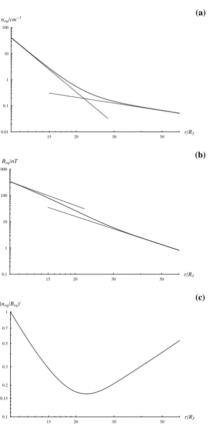
Fig. 2. Log-log plot of the “radial” profiles of the magnetic field strengthB (solid line), and the limiting plasma density within the equatorial plasma slab n∗I corresponding to the threshold of the flute instability, determined from Eq. (49) for various values ofτ (dashed lines as indicated). The parameters are shown in the “ra-dial” range 15≤ x
RJ≤50, corresponding to the Jovian middle magnetosphere, with values normalised to those at the inner edge at x
RJ=15 (B0andnI0respectively). From upper to lower, the dashed lines show the limiting density profiles forτ(the ratio of the plasma density inside and outside the plasma disk) equal to 10−5, 10−4, 10−3, and 10−2, respectively.
where the Doppler-shifted frequency for ions is, from Eqs. (2), (3b), (6), and (9)
ω0i =ω+kyV 2
ωBix
, (47)
and where we have again neglected the small Doppler shift for electrons, such thatωe0≈ω. We note that if we putτ=0 in Eq. (46) then we recover the flute mode dispersion relation derived by Bespalov and Davydenko (1994) in the limit that the medium surrounding the equatorial plasma disk is treated as a vacuum.
Substitution of Eq. (47) into Eq. (46) yields a dispersion equation which is a cubic equation for the angular frequency
ωat givenky
ω3+aω2+bω+c=0, (48)
where
a=kyV 2
ωBix
, b= −V 2
x ∂ ∂x ln
n(I0) B
!!
− τ ω 2 LH d (l−d) k2
y !
,
and
c= −kyV 2
ωBix
τ ω2LH d (l−d) k2
y !
.
The solutions of Eq. (48) consist either of three real roots, or one real root and a complex conjugate pair, one of which
corresponds to instability. The transition between these solu-tion types, corresponding to the threshold of the flute insta-bility, occurs when the discriminantDof the cubic equation is zero, that is
D= b − a2
33
27 +
2a3 27−
ab 3+
c2
4 =0, (49)
The condition for three real roots isD≤0. As can be seen, at a given positionx Eq. (49) is itself a cubic equation for the gradient∂
lnn(I0)
. B
.
∂xfor givenky, from which the limiting density profile for givenB (x)can be calculated numerically, as we now discuss.
To undertake these numerical calculations, we must first choose suitable representative values for the model parame-ters, together with the magnetic field profile. In the calcu-lations presented here we have taken the half-width of the plasma disk d=2RJ, the length of the field lines l=1.3x, and (as above) the “azimuthal” velocity of the plasma
V=15JRJ≈190 km s−1. Results will be presented for several values of the density ratio τ <1. For the magnetic field model we have taken a simple power lawB (x)∝x−β, where specificallyβ=3.8. As we will see below, this cor-responds to a typical behaviour of the equatorial magnetic field in the inner part of the middle magnetosphere, over a radial range from ∼10 to ∼30RJ. At larger distances the equatorial field falls less steeply with distance (Khurana and Kivelson, 1993). Numerical analysis then shows that the discriminant of the cubic equation given by Eq. (49) is positive, such that there is only one real solution for
∂
lnn(I0) .
B .
∂xat a givenky. This root is always neg-ative (such thatn(I0) decreases withx faster thanB), and at a givenx has a single (negative) maximum value which we denote as ∂ ln n∗IB∂x, at a wave number which we denote asky∗. For∂lnnI(0).B.∂x<∂ ln n∗IB∂x
we thus have a range of unstable modes, while for
∂lnn(I0).B.∂x>∂ ln n∗I
B
∂x there are no un-stable modes. The value of∂ ln n∗IB∂xat a givenx
thus gives the steepest density profile that is just stable to the flute mode, whilek∗ygives the flute mode wave number at this threshold of instability. The corresponding real frequency of the perturbationω∗at the threshold of instability can then be determined by substitution of these values into Eq. (48). It should be noted that the valuesω∗andk∗ymust satisfy the in-equalities given by Eqs. (16) and (44). It is found that these are satisfied only ifτ <0.1, i.e. if the plasma density outside the equatorial disk is sufficiently small compared with the disk density. The case for τ >0.1 where these approxima-tions are not appropriate will be discussed elsewhere.
Numerically calculated limiting density profiles deter-mined by integrating the∂ ln n∗IB∂xvalues are plot-ted versus xRJ
[image:8.595.50.287.557.681.2]
P. A. Bespalov et al.: Jovian magnetospheric interchange instability 2051 while the dashed lines show the density profiles for four
values of τ, namely 10−2, 10−3, 10−4 and 10−5, as indi-cated in the figure. The solutions are shown in the range of
x
RJ from 15 to 50, and the parameter values are nor-malised to the values at x
RJ=15 (B0 and nI0 respec-tively). It can be seen that for the smallest value,τ=10−5, the limiting density profile is close to the magnetic field pro-file, though falling slightly more rapidly with increasing dis-tance (i.e. ∂ ln n∗IB∂x is negative but small). This is in accordance with previous results which show that for the case of a vacuum outside the plasma disk, such that the influence of the coupling with the ionosphere is eliminated, marginal stability simply requires∂ ln n∗IB∂x=0, such that n∗IBis a constant. For very smallτ, therefore, we find thatn∗Ivery nearly follows the magnetic field profile. As
τ increases, however, the limiting profiles shown in Fig. 2 become increasingly steep, due physically to current feed-back from the conducting ionosphere which damps the in-stability, and which allows stability with larger radial den-sity gradients. The log-log profiles of the plasma denden-sity remain almost linear, however, indicating an approximate power law behaviour n∗I∝x−η. For the cases shown, we find approximately thatη∼3.94 forτ=10−5, corresponding closely to the chosen magnetic field exponent of 3.8, increas-ing to∼4.24 forτ=10−4,∼5.20 forτ=10−3, and to∼8.22 for τ=10−2. The corresponding values of k∗
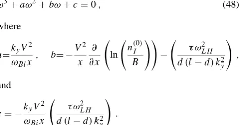
y, normalised to RJ−1, are shown versus xRJ for the same τ values in Fig. 3. It can be seen that the values correspond to “az-imuthal” wavelengths which are generally very small com-pared with the circumference around the planet at a given “ra-dius”, in conformity with the above assumptions. The corre-sponding real frequency of the perturbations,ω∗, is found to be very low, and typically lies in the interval between∼10−4 and∼10−3rad s−1.
6 Comparison with observations
It is of interest to make an initial comparison of these results with observed radial distributions of plasma in the jovian equatorial plasma disk, using density data from the Galileo spacecraft. Frank et al. (2002) have provided convenient power law fits to the density values observed within the equa-torial current sheet on Galileo orbit G08 (4 May to 22 June 1997). Data were obtained between a periapsis of∼10RJ and an apoapsis of∼100RJ, where the latter lay in the post-midnight sector of the magnetotail. It was found that the equatorial density falls very steeply with radial distance in the inner part of the system, but much less rapidly further out. For radial distances less than 20RJ they found
neq(r) ≈ 3.2×10⁸ R
J
r 6.9
cm−3, (50)
15 20 30 50
0.00001 0.0001 0.001 0.01 0.1
B/B0 t=0.01 t=0.001 t=0.0001 t=0.00001
x/RJ n nI*/I0
20 25 30 35 40 45 50
-700 -600 -500 -400 -300 -200 -100
x/RJ
t=0.01 t=0.001 t=0.0001 t=0.00001
[image:9.595.310.542.61.204.2]k Ry* J
Fig. 3. Plot of theycomponent of the flute mode wave vector (the “azimuthal” wave number), normalised toRJ−1, corresponding to the threshold of instability at the limiting density gradient shown in Fig. 2, plotted versus “radial” distancex for various values of τ. From upper to lower, the dashed lines thus showk∗yRJ versus
xRJ
forτequal to 10−5, 10−4, 10−3, and 10−2, respectively, as indicated.
while for radial distances beyond 50RJ they obtained
neq(r) ≈ 9.8 R
J
r 1.28
cm−3. (51)
Between ∼20 and ∼50RJ the density data are relatively sparse, but can reasonably be represented by an overall pro-file given by the sum of the above two propro-files. This is shown in log-log format in Fig. 4a, where the solid line shows the sum of the above two functions, while the two dashed straight lines show the power laws to which this asymptotes at small and large radial distances as given by the fits to the data. Results are shown over the radial range from 10 to 60RJ, thus overlapping the range of the theoretical results shown in Figs. 2 and 3.
The theoretical results derived in Sect. 5 above and shown in Fig. 2 concern the radial variation of the quantity nB
15 20 30 50 rêRJ 0.01
0.1 1 10 100 neqêcm-3
(a)
15 20 30 50 rêRJ 0.1
1 10 100 1000
BeqênT
(b)
15 20 30 50 rêRJ 0.1
0.15 0.2 0.3 0.5 0.7 1 HneqêBeqL'
[image:10.595.62.276.54.490.2](c)
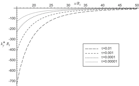
Fig. 4. Equatorial thermal plasma density and magnetic field strength profiles are shown plotted versus radial distance from Jupiter in the range from 10 to 60RJ, as determined from data ob-tained on Galileo orbit G08. The dashed straight lines in plot (a) show the power-law fits to the equatorial thermal plasma density valuesneqin the radial ranges forr<20RJ andr>50RJ, respec-tively, determined by Frank et al. (2002) and given by Eq. (50). The solid line shows their sum, taken to represent the overall den-sity profile in the radial range shown. The solid line in plot (b) shows the profile of equatorial field strength minimaBeq on the orbit, again in log-log format, represented by Eq. (52). The lower dashed line shows the second term only in Eq. (52), correspond-ing to the Khurana and Kivelson (1993) model. The upper dashed line shows the first term in Eq. (52) with the exponential term set to unity, such that the value varies with distance as the inverse cube. Plot (c) shows a log-log plot of the ratio neqBeq, normalised to its value at 10RJ.
in the radial range between∼15 and∼20RJ. The resulting field strength model is given by
Beq(r) =Bo
RJ r
3 exp
" −
r ro
2# +A
RJ
r m
,(52)
where Bo=3.335×10⁵nT, ro=17RJ , A=5.4×10⁴nT and m=2.71. The second term in this expression is the Khu-rana and Kivelson (1993) model, while the first is a modified dipole in form. Direct comparison with the G08 data shows that Eq. (52) provides a good description of the field strength minima out to at least∼60RJ, for which purpose it is em-ployed here. A log-log plot of the field profile is shown by the solid line in Fig. 4b. The lower dashed line shows the sec-ond term in Eq. (52) alone (the Khurana and Kivelson (1993) model), to which the solid curve asymptotes at distances be-yond∼35RJ. The upper dashed line shows the first term in Eq. (52) alone with the exponential set equal to unity, which thus decreases with distance as the inverse cube. It can thus be seen that over the radial range from∼10 to∼30RJ the equatorial field falls somewhat more steeply than for a dipole field, investigation of the profile showing that a power law of ∼r−3.8provides a good description.
We thus find that at radial distances between ∼10 and ∼20RJ, the equatorial field strength on orbit G08 falls as ∼r−3.8, while the plasma density determined by Frank et al. (2002) falls much more steeply as∼r−6.9. This density profile can then be compared directly with the theoretical re-sults derived in Section 5 and illustrated in Fig. 2, since an equatorial magnetic field varying as x−3.8 was specifically employed to derive those results, as noted above. Compari-son with the results in Fig. 2 then implies that the ratio of the plasma density outside and inside the current sheet is approx-imatelyτ≈0.005, a value which is in reasonable agreement e.g. with the Voyager results presented by Belcher (1983). We emphasise that such steep density profiles can exist in near-equilibrium only because of the electrical coupling of the plasma disk and the ionosphere, through the plasma that lies between. In making this simple comparison of equatorial plasma density and field strength profiles we are assuming, of course, that the plasma disk remains roughly constant in thickness over the radial range considered. However, mod-est variations in thickness will not change the nature of our conclusion. We are also assuming that the observed density profile is indeed close to the condition for marginal stability. In practice, the observed gradient might possibly represent conditions a little beyond this condition, such that slow in-terchange motions are in progress. In this case the value ofτ
might be a little lower than that estimated above.
Beyond ∼20RJ, however, the density profile in Fig. 4a falls more slowly than the field profile shown in Fig. 4b. This is shown explicitly in Fig. 4c, where we present the corresponding plot of neq
Beq
then increases again at larger distances. The latter increase may in part be due to a thinning of the plasma sheet with increasing distance, resulting in an increase in the equatorial density for fixed plasma disk content. Increasing values of
neqBeqover and above this effect are clearly not expected on the basis of the theory presented here. As pointed out in the Introduction, however, the density profile can be fur-ther smoothed beyond the threshold profile calculated here by slower instabilities, to which we may then attribute the effect found here at larger distances.
7 Summary
In this paper we have examined the flute instability of the equatorial disk of iogenic plasma in Jupiter’s middle magne-tosphere. Particular attention has been paid in the analysis to the wave coupling between the dense plasma in the equa-torial disk and the more rarefied plasma at higher latitudes, and between the latter plasma and the conducting planetary ionosphere. The analysis has been undertaken using a system with local Cartestian symmetry to simplify the geometric as-pects of the problem, with “external” forces being used to represent the acceleration of the disk plasma due to plasma rotation and to field line curvature. The local Cartesian ap-proximation is valid in the limit that the flute perturbations are of small spatial scale in the “azimuthal” direction. For such small-scale perturbations the ionosphere can also be treated as a perfect electrical conductor, and the condition under which this approximation holds has been determined.
We have then examined the conditions under which flute perturbations in this system are at the threshold of instability, and have used this to determine the corresponding limiting radial gradient of the plasma density within the plasma disk. In common with previous analyses, we find that when the density of the high-latitude plasma falls to values which are sufficiently low compared with the equatorial disk, such that coupling to the ionosphere becomes insignificant, the lim-iting density distribution follows that of the magnetic field, such that nBis a constant within the disk. However, as the density of the high-latitude plasma increases towards that of the disk, and with it the significance of the stabilising inter-action with the ionosphere, then the limiting plasma density distribution in the disk falls increasingly steeply compared with that of the magnetic field.
Initial comparison with density values obtained by the Galileo spacecraft, specifically with those observed on orbit G08 presented by Frank et al. (2002), shows that the equato-rial density falls much more steeply than the equatoequato-rial field strength in the radial distance range from∼10 to ∼20RJ. The theory presented here shows that such profiles are stable only because of the effect of the coupling of the equatorial plasma disk with the ionosphere, through the plasma that lies between. The observed profiles in this region suggest that the ratio of the plasma density inside and outside the plasma disk
is∼0.005. Beyond∼20RJ, however, the equatorial density is found to fall less steeply with distance than the equatorial field strength, suggesting the action of additional smoothing processes, together possibly with the effect of thinning of the plasma disk.
We finally note that although most of this paper has been concerned specifically with the Jovian system, similar con-siderations can also be applied in principle to Saturn’s mag-netospheric plasma environment. This problem will be ex-amined once the field and plasma environment has been suf-ficiently elucidated through examination of data from the Cassini orbiter mission.
Acknowledgements. This work was partly funded by INTAS grant
number 03-51-3922. Work at Nizhny Novgorod was also supported by RFBR grant 05-02-16350, and by the General Physics Division of the Russian Academy of Sciences (Programme “Plasma Pro-cesses in the Solar System”). Work at Leicester was also supported by PPARC grant PPA/G/O/2003/00013. Galileo magnetic field data employed in the study were obtained through the Planetary Data System at UCLA.
Topical Editor I. A. Daglis thanks J. Woch and another referee for their help in evaluating this paper.
References
Acu˜na, M. H., Behannon, K. W., and Connerney, J. E. P.: Jupiter’s magnetic field and magnetosphere, in: Physics of the Jovian Magnetosphere, edited by: Dessler, A. J., Cambridge Univ. Press, Cambridge, U.K., 1–50, 1983.
Bagenal, F.: Empirical model of the Io plasma torus – Voyager mea-surements, J. Geophys. Res., 99, 11 043–11 062, 1994.
Bagenal, F.: The ionization source near Io from Galileo wake data, Geophys. Res. Lett., 24, 2111–2114, 1997.
Bagenal, F. and Sullivan, J. D.: Direct plasma measurements in the Io torus and inner magnetosphere of Jupiter, J. Geophys. Res., 86, 8447–8466, 1981.
Belcher, J. W.: The low-energy plasma in the jovian magnetosphere, in Physics of the Jovian Magnetosphere, edited by: Dessler, A. J., Cambridge Univ. Press, Cambridge, U.K., 68–105, 1983. Bespalov, P. A. and Zheleznyakov, V. V.: Formation of disks around
hot stars under the action of radiation pressure, Sov. Astron. Lett., 16, 442–452, 1990.
Bespalov, P. A. and Davydenko, S. S.: On the structure of the plasma disk in the Jovian magnetosphere, Planet. Space Sci., 42, 583–592, 1994.
Brown, M. E.: Observations of mass loading in the Io torus, Geo-phys. Res. Lett., 21, 10, 847–850, 1994.
Bunce, E. J. and Cowley, S. W. H.: Local time asymmetry of the equatorial current sheet in Jupiter’s magnetosphere, Planet. Space Sci., 49, 261–274, 2001.
Caudal, G.: A self-consistent model of Jupiter’s magnetodisc in-cluding the effects of centrifugal force and pressure, J. Geophys. Res., 91, 4201–4221, 1986.
Cowley, S. W. H. and Bunce, E. J.: Origin of the main auroral oval in Jupiter’s coupled magnetosphere-ionosphere system, Planet. Space Sci., 49, 1067–1088, 2001.
Delamere, P. A. and Bagenal, F.: Modeling variability of plasma conditions in the Io torus, J. Geophys. Res., 108(A7), 1276, doi:10.1029/2002JA009706, 2003.
Divine, N. and Garrett, H. B.: Charged particle distributions in Jupiter’s magnetosphere, J. Geophys. Res., 88, 6889–6903, 1983. Ferri`ere, K. M. and Andr´e, N.: A mixed magnetohydrodynamic-kinetic theory of low-frequency waves and instabilities in strat-ified, gyrotropic, two-component plasmas, J. Geophys. Res., 108(A7), 1308, doi:10.1029/2003JA009883, 2003.
Frank, L. A. and Paterson, W. R.: Survey of thermal ions in the Io plasma torus with the Galileo spacecraft, J. Geophys. Res., 106, 6131–6149, 2001.
Frank, L. A. and Paterson, W. R.: Plasmas observed near local noon in Jupiter’s magnetosphere with the Galileo spacecraft, J. Geo-phys. Res., 109, A11217, doi:10.1029/2002JA009795, 2004. Frank, L. A., Paterson, W. R., and Khuarana, K. K.: Observations of
thermal plasmas in Jupiter’s magnetotail, J. Geophys. Res., 107, A11003, doi:10.1029/2001JA000077, 2002.
Goertz, C. K.: Io’s interaction with the plasma torus, J. Geo-phys. Res., 85, 2949–2956, 1980.
Gold, T.: Motions in the magnetosphere of the Earth, J. Geo-phys. Res., 64, 1219–1224, 1959.
Gurnett, D. A., Scarf, F. L., Kurth, W. S., Shaw, R. R., and Poyn-ter, R. L.: Determination of Jupiter’s electron density profile from plasma wave observations, J. Geophys. Res., 86, 8199– 8212, 1981.
Hill, T. W.: Interchange stability of a rapidly rotating magneto-sphere, Planet. Space Sci., 24, 1151–1154, 1976.
Hill, T. W.: Inertial limit on corotation, J. Geophys. Res., 84, 6554– 6558, 1979.
Hill, T. W.: The jovian auroral oval, J. Geophys. Res., 106, 8101– 8107, 2001.
Hill, T. W., Dessler, A. J., and Maher, L. J.: Corotating magneto-spheric convection, J. Geophys. Res., 86, 9020–9028, 1981. Hill, T. W., Dessler, A. J., and Goertz, C. K.: Magnetospheric
models, in Physics of the Jovian Magnetosphere, edited by: Dessler, A. J., Cambridge Univ. Press, Cambridge, U.K., 353– 394, 1983.
Huang, T. S., and Hill, T. W.: Drift-wave instability in the Io plasma torus, J. Geophys. Res., 96, 14 075–14 083, 1991.
Khurana, K. K.: Influence of solar wind on Jupiter’s magnetosphere deduced from currents in the equatorial plane, J. Geophys. Res., 106, 25999–26016, 2001.
Khurana, K. K. and Kivelson, M. G.: Inference of the angular veloc-ity of plasma in the jovian magnetosphere from the sweepback of magnetic field, J. Geophys. Res., 98, 67–79, 1993.
Kivelson, M. G., Khurana, K. K., Russell, C. T., and Walker, R. J.: Intermittent short-duration magnetic field anomalies in the Io torus: evidence for plasma interchange?, Geophys. Res. Lett., 24, 2127–2130, 1997.
Krimigis, S. M. and Roelof, E. C.: Low-energy particle population, in: Physics of the Jovian Magnetosphere, edited by: Dessler, A. J., Cambridge Univ. Press, Cambridge, U.K., 106–156, 1983. Kronberg, E. A., Woch, J., Krupp, N., Lagg, A., Khurana, K. K., and
Glassmeier, K.-H.: Mass release at Jupiter: Substorm-like pro-cesses in the jovian magnetotail, J. Geophys. Res., 110, A03211,
doi:10.1029/2004JA010777, 2005.
Liu, W. W.: Centrifugally driven instability of a rotationally domi-nated magnetodisc, J. Geophys. Res., 103, 4707–4714, 1998. Mauk, B. H. and Krimigis, S. M.: Radial force balance within
Jupiter’s dayside magnetosphere, J. Geophys. Res., 92, 9931– 9941, 1987.
Mauk, B. H., Krimigis, S. M., and Lepping, R. P.: Particle and field stress balance within a planetary magnetosphere, J. Geo-phys. Res., 90, 8253–8264, 1985.
Mauk, B. H., Gary, S. A., Kane, M., Keath, E. P., Krimigis, S. M., and Armstrong, T. P.: Hot plasma parameters of Jupiter’s inner magnetosphere, J. Geophys. Res., 101, 7685–7695, 1996. Melrose, D. B.: Rotational effects on the distribution of thermal
plasma in the magnetosphere of Jupiter, Planet. Space Sci., 15, 381–393, 1967.
Mikhailovskii, A. B.: Theory of Plasma Instabilities, Vol. 1. Insta-bilities of an Inhomogeneous Plasma, Consultants Bureau, New York, 1974.
Nichols, J. D. and Cowley, S. W. H.: Magnetosphere-ionosphere coupling currents in Jupiter’s middle magnetosphere: Effect of precipitation-induced enhancement of the ionospheric Pedersen conductivity, Ann. Geophys., 22, 1799–1827, 2004.
Pontius Jr., D. H.: Radial mass transport and rotational dynamics, J. Geophys. Res., 102, 7137–7150, 1997.
Pontius, Jr. D.H. and Hill, T.W.: Departure from corotation of the Io plasma torus: Local plasma production, Geophys. Res. Lett., 9, 1321–1324, 1982.
Pontius Jr., D.H., and Hill, T.W.: Rotation-driven plasma transport: The coupling of macroscopic and microdiffusion, J. Geophys. Res., 94, 15 041–15 053, 1989.
Pontius Jr., D.H., Hill, T. W., and Rassbach, M. E.: Steady-state plasma transport in a corotation-dominated magnetosphere, Geo-phys. Res. Lett., 13, 1097–1110, 1986.
Pontius Jr., D.H., Wolf, R. A., Hill, T. W., Spiro, R. W., Yang, Y. S., and Smyth, W. H.: Velocity shear impoundment of the Io plasma torus, J. Geophys. Res., 103, 19 935–19 946, 1998.
Sands, M. R. and McNutt, R. L.: Plasma bulk flow in Jupiter’s day-side middle magnetosphere, J. Geophys. Res., 93, 8502–8518, 1988.
Siscoe, G. L. and Summers, D.: Centrifugally-driven diffusion of iogenic plasma, J. Geophys. Res., 86, 8471–8479, 1981. Siscoe, G. L., Eviatar, A., Thorne, R. M., Richardson, J. D.,
Bage-nal, F., and Sullivan, J. D.: Ring current impoundment of the Io plasma torus, J. Geophys. Res., 86, 8480–8484, 1981.
Southwood, D. J. and Kivelson, M. G.: Magnetospheric interchange instability, J. Geophys. Res., 92, 109–116, 1987.
Southwood, D. J. and Kivelson, M. G.: Magnetospheric interchange motion, J. Geophys. Res., 94, 299–308, 1989.
Staines, K., Balogh, A., Cowley, S. W. H., Edwards, T. M., Forsyth, R. J., and Hynds, R. J.: An overview of the Anisotropy Telescope observations of MeV ions during the Ulysses Jupiter encounter, Planet. Space Sci., 44, 341–369, 1996.
Summers, D. and Siscoe, G. L.: Wave modes of the Io plasma torus, Astrophys. J., 295, 678–684, 1985.
Thorne, R. M., Armstrong, T. P., Stone, S., Williams, D. J., McEn-tire, R. W., Bolton, S. J., Gurnett, D. A., and Kivelson, M. G.: Galileo evidence for rapid interchange transport in the Io torus, Geophys. Res. Lett., 24, 2131–2134, 1997.
Jovian Magnetosphere, edited buy: Dessler, A. J., Cambridge Univ. Press, Cambridge, U.K., 395–453, 1983.
Woch, J., Krupp, N., and Lagg, A.: Particle bursts in the jovian magnetosphere: Evidence for a near-Jupiter neutral line, Geo-phys. Res. Lett., 29(7), doi:10.1029/2001GL014080, 2002.
Woch, J., Krupp, N., Lagg, A., and Tom´as, A.: The structure and dy-namics of the Jovian energetic particle distribution, Adv. Space Res., 33, 2030–2038, 2004.