The Pension Forum

F

ORUM

THE PENSION

published by the Pension Section of the Society of Actuaries

The Pension Forum is published on an ad-hoc basis by the Pension Section of the Society of

Actuaries. The procedure for submitting an article appears on page 59.

The Pension Forum is sent without charge to all members of the Pension Section.

All correspondence should be addressed to: Arthur J. Assantes

Editor, Pension Section News / The Pension Forum The Pension Section

Society of Actuaries

475 N. Martingale Road, Suite 600 Schaumburg, IL 60173

Expressions of Opinion

The Society of Actuaries assumes no responsibility for statements made or opinions expressed in the stories. Expressions of opinion are those of the writers and, unless expressly stated to the con-trary, are not the opinion or position of the Society of Actuaries or the Pension Section.

Comments on any of the papers in this Forum are welcomed. Please submit them to Art Assantes, editor. They will be published in a future issue of the Pension Section News.

Printed in the United States of America

Copyright 2004 © Society of Actuaries

The Pension

Forum

Volume 15, Number 1 December 2004

Table of Contents PAGE

Introduction to Yield Curve Forum 1

by Kenneth A. Kent, FSA, FCA

Understanding the Corporate Bond Yield Curve 2

by Holger Höfling, University of Ulm, Rüdiger Kiesel, University of Ulm and LSE Gunther Löffler, University of Ulm

Durational (Select and Ultimate) Discount Rates for FAS 87 and 106 Valuations 35

by Ron Iverson, Heidi Rackley, Steve Alpert, and Ethan Kra

Valuation of Pension Obligations with Lump Sums 46

THEPENSIONFORUM

Introduction to Yield Curve Forum

by Kenneth A. Kent, FSA, FCA

The concept of using a corporate bond yield curve for valuating pension plan liabilities explod-ed on the scene when the fexplod-ederal administration proposed using the yield curve as a means to replace the 30-year Treasury rate.

For many of us, our familiarities with the yield curve are associated with learning about forward rates and spot rates during our period of exam taking, but we have not worked with valuation systems that call for its direct application. And, it is clear the administration’s approach of applying a corporate yield curve to a simple cash flow stream is more easily said than done when work-ing with complex, multi-decrement models com-mon acom-mong pension valuation systems. Nor may they be fully considering the implications on interest-sensitive benefits and rights common in today’s pension plans.

What is of concern to members of the Society of Actuaries Pension Section Council is that actuar-ies have an understanding of the development of a corporate bond yield curve, including:

• The market basket of securities used to develop the curve,

• The quality of these securities,

• How the curve responds to changes in short-and long-term rates short-and

• How callable bonds are used and their impact if they are excluded from the curve structure.

Another important question is, if the corporate bond yield curve is the benchmark for liability calculations for pension funded status, can a sim-ilar portfolio of securities be purchased to hedge against interest rate risk?

As a first step in addressing the lack of literature that addresses this index as a viable market index to measure pension plan solvency, the Pension

Section Council called for a paper to present a review and analysis of the yield curve and the securities used to develop the curve. We are pleased to present the results of our search with the first paper in this forum, “Understanding the Corporate Bond Yield Curve,” by Holger Höfling, Rüdiger Kiesel and Gunter Löffler.

To accompany this centerpiece, we also include two papers that address some of the complex applications of a yield curve to benefits and valu-ations. Dick Wendt’s paper, “Valuation of Pension Obligations with Lump Sums,” provides insight into how to apply the curve in the valua-tion of lump sums. The yield curve could also offer some use as a tool in the valuation of expense under FAS 87 and FAS 106, as presented in the third paper prepared by Ron Iverson, Heidi Rackley, Steve Alpert and Ethan Kra titled, "Durational (Select & Ultimate) Discount Rates for FAS 87 &106 Valuations."

The appropriate application of the corporate bond yield curve may be debated for some time, even if it is ultimately deemed an appropriate means of measuring plan solvency. Regardless of debate, analysis of the yield curve offers insight into the valuation of liabilities as they relate to market interest rates and, accordingly, will contin-ue to be of interest in relation to actuarial valua-tions of pension liability.

1. Overview: Issues in Constructing the

Corporate Bond Yield Curve

The discontinuation of the 30-year Treasury rate made it necessary to introduce a new interest rate for valuing liabilities of pension funds. Current legislation proposes using a yield curve estimated from corporate bond data for this purpose.

In the literature several models are discussed that can be used to estimate yield curves: government and corporate. These methods are well docu-mented and easy to use, provided that the neces-sary data are available.1 _{The main differences in} the estimation procedure between corporate and government bond yield curves are due to issues regarding the availability and quality of the data sets used for estimation purposes.

1.1 Government Bond Yield Curve

The U.S. government bond market is very liquid, resulting in price quotes that are accurate and up to date. The number of available issues is high and dense with respect to time and maturity, so that for every time to maturity, there is a bond that matures very close to it. Especially important is that for government bonds there is almost no

default risk and all bonds are from one issuer so that uncertainty about date and amount of pay-ments is reduced. Also, most government bonds do not have any special provisions such as call fea-tures, making it possible to use only bonds with-out options for the estimation process. In sum-mary: since the quality of data sets available for U.S. government bonds is very high, yield curve estimation can be done with high accuracy.

1.2 Construction of a Corporate Bond

Yield Curve

The situation is different for corporate bonds. Compared to the U.S. government yield curve, several important new factors that influence the corporate bond yield curve arise. The most important of these factors is the default risk, that is, the risk that the issuing company is not able (or not willing) to fulfill their obligations to pay coupons and/or pay back the face value of the bond. Since corporate bond holders face this default risk (which may be significant in the case of low-rated issuers), they ask for a premium to compensate for bearing it. Further issues are a lower liquidity of the market so that an investor has the risk of not being able to sell at every point

Understanding the Corporate Bond Yield Curve

by Holger Höfling, University of Ulm Rüdiger Kiesel, University of Ulm and LSE

Gunther Löffler, University of Ulm

Abstract

This paper discusses the construction of the corporate bond yield curve and possible

applications to pension valuation. The first part addresses the mathematical theory and tools

needed to extract the yield curve from corporate bond data and the issues that arise in

contrast to the Treasury yield curve. Next, specific problems concerning the construction of

the curve are explored, for example, the number of bonds available, the quality at different

durations, etc. In the last part questions arising when applying the yield curve to pension

valuation are discussed.

THEPENSIONFORUM

in time, different tax regulations for government and corporate bonds, and a larger share of bonds with call provisions or other special features. As corporate bonds face more risk factors, investors will ask for a premium for taking on these risks. Section 2 will discuss empirical results of the importance of these risks factors and the size of their contribution to the difference between the corporate and government bond yield curve (the credit spread). It will also briefly discuss bonds that include options, especially call options.

For constructing the yield curve, the data have to be sorted by the default risk of the company and whether the bonds include special options. Data on how many bonds are available for the different default risk classes — with and without options — and how the time to maturity is distributed are given in Section 3. After that, the quality of the yield curve, its behavior with respect to the inter-est rate environment, and the slope of the curve are discussed. The section ends with a discussion on bond indices and how they could be used to make valuation easier for small pension funds, as well as a description on alternative data sources for construction of a yield curve.

1.3 Application to Pension Funds

Section 4 discusses how the corporate bond yield curve might be applied in pension valuation and estimates what the effects would be in contrast to current legislation. Particular issues are interest-sensitive payment forms, cash-balance plans, and embedded options. It also discusses theoretical issues in smoothing rates of a corporate bond yield curve.

2. Credit Spread

When comparing a corporate and a government bond yield curve, one notices that the corporate bond yield curve is significantly higher than the government bond yield. The difference between these two curves is called the credit spread. The interest rate on government bonds is seen as the

riskless interest rate, so that the credit spread can be viewed as the premium that investors ask for because of additional risks of corporate bonds. This section will first discuss the size of the cred-it spread, then give possible explanations and evaluation their importance.

2.1 Size of the Credit Spread

When estimating the yield curve for corporate and Treasury bonds, the yields on corporate bonds are significantly higher. One of the main reasons for this observed credit spread are credit risk and a risk premium that investors ask for tak-ing on this risk. Here credit risk refers to the pos-sibility that a company might default or that the rating of the company worsens, so that the bond loses value. Further factors responsible for the spread are options included in the bond, decreased (as compared to Treasury bonds) liquid-ity, and taxes.

The data are average spot rates from 1992 to 1996, computed using bond data from the Fixed Income Database at the University of Houston. For more information on how the estimates were obtained see Elton et al. (2001).

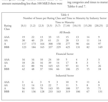
While looking at the spreads, one notices how dif-ferently the credit spread changes with the rating category for financial and industrial bonds. For rating categories AA and A, the spread for indus-trial bonds is smaller; however, for BBB the spread for financials is smaller. One explanation for this behavior is different probabilities for cred-it rating changes. Nickell, Perraudin, and Varotto (1998) show in their analysis that the probability for downgrades for AAA, AA, and A is higher for financial than for industrial bonds, and the prob-ability for upgrades is about the same. For BBBs it is the other way around: the probability for upgrades is higher, and the downgrade probabili-ty is almost identical. Another consideration is the low number of bonds issued by BBB financial companies (see Table 4). This also has been noted in Nickell, Perraudin, and Varotto (1998) and attributed to problems of running a bank if market confidence in the institution is low. Regulatory requirements might be another reason for the dif-ferent credit rating transition probabilities.

2.2 Callability

Like Treasury bonds, corporate bonds are fre-quently callable, and this option in the bond changes the price. As this option is an additional risk for the bond holder, he or she wants a yield premium. Therefore, before constructing a yield curve the "option to call" has to be priced, and the yield curve should be adjusted according-ly. However, trying to account for the call option price is difficult and could introduce significant additional noise to the price of the bond. For recent advances into pricing of callable debt and some empirical analysis, see, for example, Berndt (2003), King (2002), and Duffee (1998).

Duffee (1998) states that callable bonds are much more sensitive to interest rate movements than are noncallable bonds. In his study he found that the credit spread on corporate bonds decreases with an increasing interest rate. As a call option on debt has a lower value for the issuer with rising interest rates, the spread on callable bonds decreases faster for increasing interest rates than it does for noncallable bonds.

King (2002) empirically analyzes the behavior of call option values in relation to the height and slope of the yield curve, interest rate volatility, industry group, rating of issuer, callable period or

Table 1

Credit Spread by Time to Maturity and Rating Class

Maturity Treasury Spot Rates Financial Sector Industrial Sector

AA A BBB AA A BBB

2 5.265 0.467 0.582 0.857 0.392 0.536 1.022

3 5.616 0.501 0.640 0.899 0.396 0.580 1.070

4 5.916 0.511 0.676 0.928 0.406 0.606 1.072

5 6.150 0.512 0.701 0.948 0.415 0.623 1.062

6 6.326 0.511 0.718 0.962 0.423 0.634 1.049

7 6.461 0.510 0.731 0.973 0.429 0.642 1.039

8 6.565 0.508 0.740 0.981 0.434 0.649 1.030

9 6.647 0.507 0.748 0.987 0.438 0.653 1.022

THEPENSIONFORUM

not, and call strategy of the issuer. All of these factors have a significant influence on the price of the call option. The height and slope of the yield curve especially are important. For example, when the short-term interest rate is about 3-4%, the yield curve has a steep slope, and interest rate volatility is high, the value of the call option is about 7.15% of the par value of the bond if the bond is in its callable period. On the other hand, for high short-term interest rates (>7%), flat yield curves, and low interest rate volatility, the value of the call option is about zero. However, call values are generally low if the remaining call protection period is longer than one year. This shows that to use callable bonds for yield curve estimation, some care and an estimate of the yield curve is needed. Several models are available that could be used to compute theoretical call option values. Because of these problems, callable bonds are usu-ally excluded from estimation of yield curves in the scientific literature. The problems in valuing put options are similar, although the question has not been addressed as much as for call options. As the value of convertible bonds depends on the value of the underlying stock, these bonds are usually excluded as well. In our data set, about one-third of the bonds were callable. More infor-mation can be found below.

2.3 Default Risk

Corporations face a significantly higher default risk than do governments, which introduces a sig-nificant default risk for corporate bonds and has the effect that they are traded with a price dis-count in comparison to otherwise equivalent

Treasury bonds. This discount varies from corpo-ration to corpocorpo-ration because of different default risks. For estimating the yield curve, companies should have a comparable risk class. One way to do this is to use rating classes as an indicator for default risk. Then the estimation of the yield curve is made using only bonds of companies with a certain rating category, say, AA or A, pro-vided by one of the major rating companies.

When valuing liabilities, one should also account for default risk. When investing the amount equivalent to discounted liabilities, one probably would not be able to service the liabilities because some bonds in the portfolio will default. In Elton et al. (2001) the authors suggest a simple method to estimate the rate spread due to default risk.2

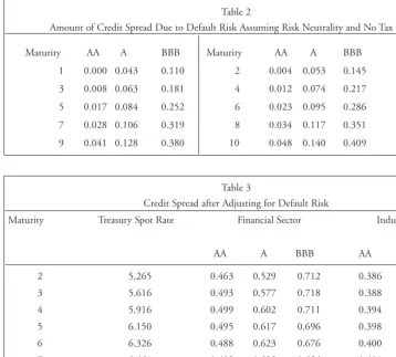
However, as Elton et al. (2001) find, only about 10% of the credit spread for AA-rated companies is due to default risk, 20% for A-rated and 40% for BBB-rated bonds. The credit spread due to default risk assuming risk neutrality and no tax effects as estimated by Elton et al. (2001) can be found in Table 2. The credit spreads after adjust-ing for this default risk are shown in Table 3, and a graphical comparison of spot rates for Treasury and A-rated industrial bonds is shown in Figure 1. These findings are qualitatively confirmed by the more extensive analysis in Huang and Huang (2003). They calibrate most commonly used and analytically tractable structural credit risk models to historical data and calculate the percentage of credit spread due to credit risk (including a pre-mium for taking on this risk) explained by the

2 _{Let a be the constant fraction of the face value of the bond paid upon default. Let P}

tbe the probability of default in period t conditional on no default earlier. Let C be the constant coupon of the bond with face value 1, and rC _{and r}G _{denote the}

cor-porate and government forward rate from period t to t + 1 , where the government rate is known. Then the rate spread due to default risk can be obtained recursively using the equations

where VtTdenotes the value of the bond at time t, maturing at T. The probabilities and the recovery fraction are taken from transition matrices and recovery fraction tables provided by the major rating companies. The government rate is obtained by yield curve estimation using government bond data. Of course, there are several other ways to account for this default risk. Another possibility would be to use a structural or reduced form model. For an extensive empirical analysis using structural mod-els see Huang and Huang (2003). For an introduction to structural and reduced form modmod-els see Bingham and Kiesel (2004).

models. They find that for bonds with an AAA, AA, or A rating and 10 years to maturity, the credit spread implied by these models is only about 20% of the actual observed credit spread. For BBB-rated bonds, this percentage increases to 30%. The percentage explained increases for lower-rated companies and decreases for bonds with shorter maturities.

Kiesel, Perraudin, and Taylor (2003) point out that especially for an investment-grade bond portfolio, changing credit quality (due to rating changes) has a significant impact on the observed credit spreads. This shows that even if the yields are adjusted for default risk, which should be done for valuing liabilities, the majority of the credit spread remains.

Table 2

Amount of Credit Spread Due to Default Risk Assuming Risk Neutrality and No Tax Effects

Maturity AA A BBB Maturity AA A BBB

1 0.000 0.043 0.110 2 0.004 0.053 0.145

3 0.008 0.063 0.181 4 0.012 0.074 0.217

5 0.017 0.084 0.252 6 0.023 0.095 0.286

7 0.028 0.106 0.319 8 0.034 0.117 0.351

9 0.041 0.128 0.380 10 0.048 0.140 0.409

Table 3

Credit Spread after Adjusting for Default Risk

Maturity Treasury Spot Rate Financial Sector Industrial Sector

AA A BBB AA A BBB

2 5.265 0.463 0.529 0.712 0.386 0.483 0.877

3 5.616 0.493 0.577 0.718 0.388 0.517 0.889

4 5.916 0.499 0.602 0.711 0.394 0.532 0.855

5 6.150 0.495 0.617 0.696 0.398 0.539 0.807

6 6.326 0.488 0.623 0.676 0.400 0.539 0.763

7 6.461 0.482 0.625 0.654 0.401 0.536 0.720

8 6.565 0.474 0.623 0.630 0.400 0.532 0.679

9 6.647 0.466 0.620 0.607 0.397 0.525 0.642

10 6.713 0.458 0.614 0.584 0.393 0.517 0.607

THEPENSIONFORUM

2.4 Liquidity

Two sources of pricing errors are related to bond liquidity. The first is a price discount for corpo-rate bonds that do not have much liquidity. For bond holders, lack of liquidity introduces the risk that they might not be able to sell the bond at the time they want to. For this risk they expect a pre-mium, which leads to a discount on the price. The second kind is called a stale price error. The bond prices usually are averages of dealer quotes. For bonds with a low liquidity, dealers might not update their quotes regularly because there is not much business to attract. This can result in prices that no longer reflect the market prices. Recently several papers have addressed these problems.

Diaz and Skinner (2001) regress yield errors of their analysis on proxies for liquidity like issue size and relative age of the bond. They show that the issue size is not a significant proxy for liquidity, which they attribute to the fact that they used only bonds included in the Lehman Brothers indices. These bonds must have a minimum issue size of 50 Mill.$ (starting 1989). The relative age of the bond, however, is clearly significant for the pricing error. For bonds that are close to maturi-ty, the credit spread increases by several basis points (2-5 basis points per standard deviation change in relative age).

Another analysis was conducted by Perraudin and Taylor (2002). They find that liquidity plays an important role in determining credit spreads and that a substantial portion of the credit spread (up to 30 basis points, which is 30% to over 50% depending on rating class) for investment-grade bonds can be attributed to it. However, it is hard to find exact figures on how much of the credit spread can be attributed to liquidity. Often papers state just that the liquidity proxies are significant, but not the size of their effect.

2.5 Taxes

Another source for credit spreads is taxes. Treasury bonds are subject only to federal taxes, while corporate bonds are also subject to state taxes. As an investor earns only interest reduced by taxes, the lower earnings on otherwise equiva-lent bonds due to taxes lead to a premium for cor-porate bonds. Detailed information on how the authors adjust for taxes can be found in Elton et al. (2001), Delianedis and Geske (2001), Perraudin and Taylor (2002), or McCulloch (1971). We will just present some of the results of Elton et al. (2001).

In Elton et al. (2001) the authors assume the investor's federal tax rate to be t_g= 35% and a state tax rate of t_s= 7.5%. This leads to a margin-al state tax rate of t_s(1 - t_g) = 4.875%. This mar-ginal tax rate minimizes the squared pricing error. With these figures they estimate that the credit spread due to taxes is about 35 basis points for all maturities, which would explain about 55% of the credit spread for Arated bonds, 35% for A-rated, and almost 25% for BBB-rated.

This shows that taxes account for a large part of the corporate-Treasury spread — especially for high-quality bonds. However, not all of the credit spread is explained by default risk, taxes, or liquidity.

2.6 Risk Premium

3. Issues in the Construction of the

Corporate Bond Yield Curve

3.1 Depth

The data used for this section were obtained from Datastream3 _{and analyzed using S-Plus.}4 _We

obtained data from 10,610 corporate bonds, traded in the United States and denominated in U.S. dol-lars, 3,162 being in the financial sector and 7,448 in the industrial sector. Government and mortgage bonds were excluded. After sorting out bonds that were callable, convertible, putable, or had sinking funds, no recent price, no current rating, no invest-ment-grade rating, variable interest rates, or an amount outstanding less than 100 Mill.$ there were

4,026 bonds were left, 1,403 from the financial sec-tor and 2,623 from the industrial secsec-tor. In terms of the amount of bonds issued, the data set included bonds with a face value of 4,399,979 Mill.$, 1,186,625 Mill.$ from the financial and 3,213,355 Mill.$ from the industrial sector. After the sorting process, bonds with a face value of 1,388,856 Mill.$ were left, 525,652 Mill.$ in financial and 863,204 Mill.$ in industrial-sector bonds.

The number of bonds for different rating categories and times to maturity is reported in Tables 4 and 5 and compared in Figure 2. The number of bonds outstanding in terms of face value for different rat-ing categories and times to maturity is reported in Tables 6 and 7.

3 _{A product of Thomson Financial} 4 _{A product of Insightful.}

Table 4

Number of Issues per Rating Class and Time to Maturity by Industry Sector Time to Maturity

Rating [0,1) [1,2) [2,3) [3,5) [5,7) [7,10) [10,15) [15,20) [20,25) [25,30) [30,inf )

Class

All Bonds

AAA 19 22 13 33 13 15 13 14 9 3 2

AA 30 40 29 61 21 28 13 11 14 14 5

A 117 173 164 308 158 277 98 64 97 104 42

BBB 123 184 165 337 229 425 131 82 149 142 35

Financial Sector

AAA 16 16 10 24 10 5 4 3 3 1 2

AA 18 26 16 39 14 17 8 3 5 10 2

A 61 80 94 165 63 97 41 9 26 19 8

BBB 42 48 37 104 66 106 25 15 18 25 2

Industrial Sector

AAA 3 6 3 9 3 10 9 11 6 2 0

AA 12 14 13 22 7 11 5 8 9 4 3

A 56 93 70 143 95 180 57 55 71 85 34

BBB 81 136 128 233 163 319 106 67 131 117 33

Table 5

Number of Issues by Rating Category

Bond Type BBB A AA AAA

All bonds 2002 1602 266 156

Financial 488 663 158 94

THEPENSIONFORUM

Table 6

Amount of Face Value of Issues per Rating class and Time to Maturity by Industry Sector in Mill.$

Time to Maturity

Rating [0,1) [1,2) [2,3) [3,5) [5,7) [7,10) [10,15) [15,20) [20,25) [25,30) [30,inf )

Class

All Bonds

AAA 8,470 9,692 6,361 14,280 4,819 12,915 3,321 3,357 2,693 1,550 475

AA 10,127 11,267 11,436 27,437 6,929 12,228 4,625 3,248 3,931 5,550 1,236

A 34,249 50,309 56,719 104,688 61,386 118,787 33,642 14,827 25,834 44,109 10,718

BBB 29,455 50,390 58,847 106,426 77,404 170,501 34,217 21,839 39,439 70,659 8,463

Financial Sector

AAA 7,195 7,212 5,561 11,530 4,333 4,700 600 834 400 750 475

AA 5,475 6,300 6,400 17,488 3,975 7,150 2,650 650 1,050 3,850 350

A 18,503 25,398 33,020 65,481 30,270 48,236 18,603 2,405 9,120 10,725 2,140

BBB 9,147 13,321 14,911 32,860 22,082 38,091 5,345 3,791 4,525 18,150 600

Industrial Sector

AAA 1,275 2,480 800 2,750 486 8,215 2,721 2,523 2,293 800 0

AA 4,562 4,967 5,036 9,949 2,954 5,078 1,975 2,598 2,881 1,700 886

A 15,746 24,911 23,699 39,207 31,116 70,551 15,038 12,422 16,714 33,384 8,578

BBB 20,308 37,069 43,937 73,567 55,322 132,410 28,872 18,048 34,914 52,509 7,863

In addition, one could also consider using callable bonds in the construction of a corporate bond yield curve. Altogether we had 3,644 callable bonds with a face value of 1,139,444 Mill.$, 621 (face value 215,928 Mill.$) financial and 3,023 (face value 923,516 Mill.$) industrial bonds. In Tables 8 and 9, we show these figures split up by their rating. However, after sorting the bonds using the criteria mentioned above, only 351 (121,350 Mill.$) bonds are left, 158 (59,197 Mill.$) financial and 193 (62,154 Mill.$) indus-trial-sector bonds. As these figures are rather low, we do not report them in more detail. The main reason for this low number (apart from unavail-able ratings) is that most callunavail-able bonds have a speculative grade rating. One reason for this could be that in the currently rather low interest rate environment, mainly issuers with a low rat-ing can hope for lower interest rates on their bonds (by getting a better rating), and therefore mainly they have a strong interest in being able to call the bonds.

It should be noted that we had only rating data from Standard & Poor’s available, so these num-bers are a lower boundary for the numnum-bers and capitalization of bonds available (2,645 bonds with a face value of 1,049,224 Mill.$ did not have a current Standard & Poor’s rating).

To estimate a yield curve, one has to use bonds with ratings of AA or lower because there are not very many bonds in the AAA rating category, espe-cially at the long end of the yield curve. Mixing rating categories is not a feasible option, as this will lead to large pricing errors and make it harder to adjust for default risk (see Elton et al. 2001). In addition, mixing the AAA with the AA rating

cat-Table 8

Number of Callable Bonds by Rating Category

Bond Type NR D C CC CCC B BB BBB A AA AAA

All Bonds 1412 39 6 28 267 921 330 302 279 29 31

Financial 220 3 1 2 16 73 40 107 133 14 12

Industrial 1192 36 5 26 251 848 290 195 146 15 19

Table 9

Amount of Face Value of Callable Bonds by Rating Category in Mill.$

Bond Type NR D C CC CCC B BB BBB A AA AAA

All Bonds 385,301 9,416 1,835 5,875 82,689 262,564 104,364 118,024 142,472 16,480 10,425

Financial 68,530 601 198 317 5,854 20,148 9,103 29,239 69,422 7,710 4,806

Industrial 316,276 8,815 1,637 5,558 76,835 242,416 95,261 88,785 73,050 8,770 5,619

Table 7

Amount of Face Value by Rating Category in Mill.$

Bond Type BBB A AA AAA

All bonds 667,640 555,267 98,014 67,935

Financial 162,822 263,901 55,338 43,591

THEPENSIONFORUM

egory would affect only the short end of the AA yield curve but hardly the long end, as almost no AAA bonds have a long time to maturity.

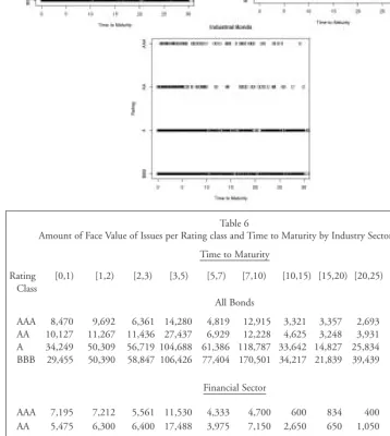
Of course, one faces the problem of the weight of one company in the estimation of the yield curve. The weight of a single company should not be too large because the company's problems would influence the yield curve estimation too much. In Tables 10 and 11,5 _{we see that in the case of}

AAA-rated bonds, the largest company accounts for 13% of the number of bonds used. If we are looking just at the financial sector, it is even more — 20%. For AA-rated bonds, the biggest issuer accounts for about 6%, 3% for A-rated, and 1% for BBBs. In terms of the amount of

outstanding bonds, the picture is even worse: 19% for AAA-rated bonds, 9% for AAs, 4% for As and 2% for BBBs. The weight of the biggest issuer is very high for AAAs, still high for AAs, and becomes negligible for lower-rated bonds. When looking at just one sector, the situation becomes worse in general.

3.2 Quality of the Curve at Different

Durations

One way of describing the quality of the curve is to measure how well discounting future payoffs using the yield curve recovers the actual market price of the bond, or, what is the size of the dif-ference between the market yield and the model yield on the bond.

Table 10

Biggest Five Issuers per Rating Category by Sector

BBB A AA AAA

All Bonds All

21 38 16 19

19 30 13 14

19 27 12 7

16 23 10 6

16 22 10 6

Financial Sector

13 38 16 19

12 30 12 14

11 27 9 6

11 20 8 6

9 15 8 5

Industrial Sector

20 23 13 7

19 22 10 7

19 19 7 6

16 14 7 6

16 13 6 5

Table 11

Biggest Five Issuers (in Terms of Face Value) per Rating Category by Sector

BBB A AA AAA

All Bonds All

13,879 19,545 7,838 13,065

13,475 12,385 6,500 6,600

8,441 10,815 5,050 5,000

7,990 10,495 4,900 3,400

6,400 9,700 4,550 3,100

Financial Sector

13,475 19,545 6,500 13,065

6,729 12,385 5,050 6,600

5,498 10,815 3,100 2,275

5,200 9,700 2,800 2,085

4,885 9,150 2,450 2,040

Industrial Sector

8,441 10,495 7,838 5,000

7,990 8,050 4,900 3,400

7,150 7,600 4,550 3,100

6,400 7,100 2,750 2,625

6,100 5,000 2,200 2,167

5 _{Inconsistencies between the tables for all bonds and the tables for financial and industrial bonds occur because Datastream}

It is hard to find exact numbers on the pricing error of corporate bonds for different durations. Pricing errors for different durations are available only for government bonds. Overall pricing errors averaged over all durations are available for gov-ernment and corporate bonds.

For government bonds we see in Bliss (1996) that the average absolute pricing error of a $100 bond increases from $0.01 for maturities up to 1 year to $0.7 for maturities over 10 years. Bonds with long time to maturity are harder to price accurately than bonds that are close to maturity.

From Elton et al. (2001) we know that the aver-age root-mean-squared error (RMSE) for treasur-ies is $0.2 per $100 face value. For corporate bonds, the RMSE is $0.5 for AAs, $0.9 for As, and $1.2 for BBBs. The results presented in Diaz and Skinner (2001) for the errors in the yield of the bonds are similar. The RMSE for the yield on treasuries is 0.0002, compared with the RMSE for AA corporate bonds, which is 0.001, five times as big. Thus, pricing errors for corporate bonds are higher than the pricing errors for gov-ernment bonds, which is not surprising as there are more unaccounted for sources of risk (e.g., different issuers, etc.). However, these pricing errors have to be interpreted with a bit of caution. Because of the mentioned unaccounted factors and pricing variability for bonds due to imperfect markets, no yield curve method gives zero error. Even for one method, increasing the number of bonds used for estimation does not necessarily lead to lower pricing errors. To some extent, these pricing errors just reflect the variability of bond prices in the market. With bond portfolios one has to consider how they behave in relation to each other. First, negative and positive pricing errors tend to cancel each other out. But, depending on the method used, it is possible that the errors have a structure, for example, the pric-ing errors for bonds with a long time to maturity all have the same sign, and the errors for

short-term bonds have the opposite sign. This structur-al effect could structur-also occur for bonds of one indus-try group or one issuer. It also depends on the estimation method and possibly other factors such as the current interest rate environment. In this case the value of liabilities could significantly deviate from the value of a bond portfolio with payouts that match the liabilities perfectly. Apart from this, one should note that the pricing error for different times to maturity will depend strongly on the minimization criterion in the yield curve estimation technique and what kinds of weights were used. In most studies the inverse of the duration of the bond was used as weight, where the error was measured as the difference of the actual and the model price. This means that less weight is put on long-term bonds.6

Therefore, the pricing error for bonds with long times to maturity will be larger than the error for short-term bonds. Thus, when estimating the spot rate curve for pension valuation purposes, a weighting scheme that puts more emphasis on long-term bonds (e.g., constant weight for all bonds) might be better.

In addition to the pricing (or yield) error, one can also consider the stability of the estimate of the yield curve — in the sense of how much the curve would be affected by an additional error in one or several bonds. This also depends on the estima-tion method used, but as a general rule one can say that the more bonds are used in the estimation process, the more stable the curve will be.

3.3 Sensitivity Issues

An important question is how sensitive corporate bonds are to the interest rate environment. The corporate bond yield curve consists of the Treasury yield curve and the credit spread curve. So, depending on how much and in which direc-tion credit spreads evolve, the corporate bond yield curve will move more or less closely with the Treasury yield curve. Duffee (1998) states that, with increasing interest rates, the spreads for

THEPENSIONFORUM

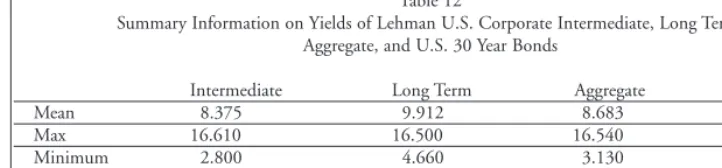
noncallable AA bonds decrease by about 15% of the amount that the Treasury rates increase. Thus, the corporate bond yield curve moves in the same direction as the Treasury yield curve, but not quite as much. To illustrate the movement of cor-porate bond rates in comparison to Treasury rates, we compared the yields on the Lehman U.S. Corporate AA Long Term, Lehman U.S. Corporate AA Intermediate, and Lehman U.S. Corporate AA Aggregate Index to the yield on the 30-year Treasury bond. The data we used con-tained the yields at the end of every month, start-ing January 1980. Some summary data can be found in Table 12. In Figure 3 one can see the monthly changes in the yield on the Lehman U.S. Corporate AA Intermediate Index in comparison to the changes in the yield on 30-year Treasury bonds. Figure 4 shows the same for the long-term index. One can see that the long-term corporate bond rate changes more closely than the interme-diate-term corporate bond rate. In Figure 5 we show the absolute value of the long-term corpo-rate bond index yields in comparison to the Treasury bond yields. It shows a quite straight line, except at the lower end. These deviating observations are all very recent and thus probably due to problems with the 30-year Treasury rate.

Another issue is how interest rates react to the market environment. Elton et al. (2001) show that the risk premium is to a large percentage determined by the Fama-French factors, intro-duced in Fama and French (1993), which are

−2 −1 0 1 2

−1.5

−1.0

−0.5

0.0

0.5

1.0

Monthly Change in Yields in percentage points

LEHMAN US CORPORATE AA LONG TERM

US Treasury 30−years

6 8 10 12 14 16

4

68

1

0

12

14

Yields on Long Term Bonds and Treasuries

LEHMAN US CORPORATE AA LONG TERM

US Treasury 30−years

Figure 3—Monthly Yield Changes of Lehman U.S. Corporate Intermediate vs. 30-Year Treasury Rate

Figure 4—Monthly Yield Changes of Lehman U.S. Corporate Long Term vs. 30-Year Treasury Rate

Figure 5—Yields of Lehman U.S. Corporate Long Term vs. 30-Year Treasury Rate

three indices that describe systematic risk in the stock market. This means that if the systematic risk in the stock market measured by these factors increases, the risk premium and thus the corpo-rate bond yield curve would increase.

3.4 Curve Behavior

As we have seen above, the Treasury yield curve and the corporate bond yield curve move very closely. This can also be seen in Figure 6. Here we used the yields on the Merrill Lynch AA-rated Corporate Bond Index with times to maturity of 1-3 years and 10-15 years and the Merrill Lynch Government Bond Index for 1-3 years and 10-15 years to matu-rity. We calculated the difference of the yields for the 10-15 year indices and the 1-3 year indices to get a proxy for the slope of the yield curves. We then plotted the proxies for the government slope against the proxy for the corporate slope. For the Treasury yield curve, data from Datastream indicate that dur-ing the last few years, yield curve inversions occurred only for a few months in 2000. The data presented above suggest that this is also true for the corporate bond yield curve. However, we did not compute the corporate bond yield curve explicitly for this time period, so we cannot verify this statement directly.

Another issue is how the yield spread depends on the time to maturity. From the spread data presented earlier, we can see that for AA-rated bonds, the spread increases with time to maturity. However, we can also observe that for other rating categories, the spread is upward sloping at the short end but down-ward sloping at the long end of the curve.

3.5 Determinants of Credit Spreads

As mentioned above, the most important factors explaining the credit spread are default risk, taxes, risk premium, and liquidity. The default risk of a company is measured using rating categories. The credit spread due to default risk is higher the lower the rating of the company is. Default risk is responsible for 10% up to 40% for AA- to BBB-rated companies. Another reason for the spread is the different tax regulations for corporate and Treasury bonds. For corporate bonds the investor has to pay taxes on the state level, from which Treasury bonds are exempt. Taxes explain 55%-25% of the spread for AA to BBB bonds. The rest of the spread can be attributed to risk premium and liquidity. Liquidity certainly plays a role, but the size of its effect is probably quite small — up to a few basis points. The remaining spread after adjusting for the other factors is explained in large part by proxies for systematic risk factors in the stock market. All in all, these four components explain most of the credit spread. However, one should note that the variables used above have only limited power to explain monthly changes in the spreads of corporate bonds. These changes are driven by another, still unknown factor. In Collin-Dufresne, Goldstein, and Martin (2001), the authors suggest that these changes are driven by local supply/demand shocks.

3.6 Bond Indices

When looking at bond indices, one should note especially two issues. First, if callable bonds are included in the index, the yield on this index will be

Note: SD of ∆Y is the standard deviation of the annual change of the yeild.

Table 12

Summary Information on Yields of Lehman U.S. Corporate Intermediate, Long Term, Aggregate, and U.S. 30 Year Bonds

Intermediate Long Term Aggregate Treasury

Mean 8.375 9.912 8.683 8.190

Max 16.610 16.500 16.540 15.171

Minimum 2.800 4.660 3.130 4.361

SD of ∆Y (per year) 1.475 1.435 1.371 1.242

THEPENSIONFORUM

higher than the yield for an otherwise equivalent index containing only noncallable bonds. Furthermore, the index will react more weakly to interest rate changes. When interest rates are increasing, the call option loses its value, and this reduces the additional spread due to the call option. Thus, the yield on the index will increase less than the yield on an index of noncallable bonds.

As an example with special application to the pen-sion system, we discuss the Citigroup Penpen-sion Liability Index.7 _{This index is created in two steps.}

First, a yield curve for AA-rated corporate bonds is derived. Then this yield curve is applied to a typi-cal pension liability profile.

For the yield curve the Treasury yield curve is derived first. The reason is that the Treasury mar-ket has a very large amount of outstanding bonds and is very liquid. This allows one to get a stable estimate for the spot rate curve. Then the par yield curve (the coupon required for a bond with a cer-tain maturity so that it trades at par) is calculated from these data (this is a unique transformation — no information is lost). The average spread of cor-porate AA bonds over Treasury bonds for a certain maturity is added to the Treasury par yield curve. This estimate of a AA corporate bond par yield curve is then transformed back into a spot rate curve (which gives the yield on a zero-coupon bond). To estimate the spreads on coupon bonds, they also use callable bonds, adjusted for the price of the call option. As they have a Treasury yield curve, there are various theoretical models available that can be used to adjust for the value of the call option. However, to reduce volatility of the call option price, they restrict themselves to callable bonds that have at least three years of call protection left and have a spread of at least 10 points between the earliest call price and its market price.

Afterwards, they apply this spot rate curve to the valuation of a typical pension liability portfolio and report the average duration and the average

annualized yield on this portfolio. For pension funds whose liability profile is similar to the one used by Citigroup, this single annualized yield can be used as a discount factor and will give very similar results to what one would get if the liabil-ities of the plan were discounted using the whole spot rate curve. However, this is not the case for pension plans with a different liability profile. Such plans should use the whole spot rate curve for their liability valuation (which is being pub-lished as well). More information can be found in Bader (1994) and Bader and Ma (1995).

3.7 Credit Default Swap Spread Curves

Recently much research on the relationship between default-free interest rates, default-risky interest rates, and default swap rates has been done. See, for example, Hull, Predescu, and White (2003), Hull, Nelken, and White (2003), Houweling and Vorst (2001), Longstaff, Mithal, and Neis (2003), and Blanco, Brennan, and Marsh (2003). The main issues these papers address is whether the credit spread is close to the default swap rate and how default swap rates behave with respect to changes in credit ratings. The main problem in determining the credit spread of a bond is the choice of the risk-free rate. Usually bond traders use the Treasury yield curve as the risk-free rate. However, a few problems exist with this rate. The main issues are the quite high spread of AAA bonds, different tax regimes, and different regulations for financial institutions that hold government and corporate bonds. Therefore, another popular choice for the risk-free rate is the swap zero curve, which is calculat-ed from LIBOR deposit rates, Eurodollar futures, and swap rates. These rates are liquid with a low credit risk and are also usually higher than the corresponding Treasury rate.

The papers mentioned above use different choic-es for the risk-free rate. Longstaff, Mithal, and Neis (2003) use the Treasury rate. They find that the default swap rate is significantly lower than

the rate implied by the credit spread (using a simple reduced form model). These findings are consistent with the analyses of Houweling and Vorst (2001) and Hull, Predescu, and White (2003). They state that using the swap rate as the risk-free rate reduces the difference between the default swap rate and the credit spread. More specifically the default-free interest rate implied by the default swap rate lies between the Treasury rate and the swap rate, about 83% of the way from the Treasury rate to the swap rate. This shows that the risk-free rate used by the market is the swap rate. The Treasury rate is perceived by the market to be too low.

Longstaff, Mithal, and Neis (2003) further ana-lyzed the difference between the credit spread on the bond and the default swap rate for the same company. They found that it varies between 12 and 100 bps for different companies and can be explained at least in part by different liquidity for the companies. With respect to changes in credit ratings, Hull, Predescu, and White (2003) find that negative changes in the ratings can be predict-ed by rising default swap rates. These results are much weaker for positive changes in credit ratings.

3.8 Emerging Market Bonds

In addition to corporate bonds, emerging market bonds may be considered. However, analyzing the credit spreads observed in the market for these bonds proves even more involved than for Treasuries. The main reason for this increased com-plexity is the additional impact that macroeconom-ic factors (inflation, exchange rates, commodity prices, etc.) and political factors (stability of gov-ernments) has on the bond price movements.

4. Applications of a Corporate Bond

Yield Curve in Pension Liability

Management

4.1 How the Yield Curve is Applied in

Pension Valuation

4.1.1 Economic Assumptions

The most important economic and actuarial assumptions in the context of pension valuation are the inflation rate, investment return rate, count rate, and compensation scale. Here we dis-cuss the economic assumptions with regard to the use of the corporate bond yield curve to obtain the discount rate. During our discussion we do not distinguish between the investment return rate and the discount rate.

When valuing pension liabilities using a yield curve, different discount rates for each future cash-flow date are used. The discount appropriate for a point in time n years from now is

e

e

n

THEPENSIONFORUM

Table 13

Life Annuity Values, Starting at Age 65, for Varying Interest Rate Scenarios

Age (1) (2) Scenario (3) (4) Change 2-1 Change 3-1 Change 4-1

80 7.03 7.24 6.79 7.41 3.00% -3.44% 5.41%

75 8.68 8.84 8.31 9.09 1.80 -4.26 4.72

70 10.34 10.36 9.81 10.71 0.18 -5.11 3.60

65 11.93 11.73 11.22 12.20 -1.66 -5.95 2.21

60 8.94 8.25 8.10 8.78 -7.71 -9.44 -1.79

50 5.26 3.89 4.42 4.35 -26.14 -16.05 -17.34

40 3.16 1.94 2.46 2.28 -38.63 -22.17 -27.73

30 1.91 1.01 1.38 1.25 -47.09 -27.84 -34.49

20 1.16 0.53 0.77 0.69 -54.38 -33.10 -40.62

forward rate minus a historically justified premium for default risk (if not already adjusted for that), risk premium, and real risk-free rate of return. Some care should be taken so that the resulting inflation rates do not become negative. One could address this by subtracting a certain percentage instead of a constant from the forward rate.

Constructing the compensation scale by combin-ing inflation, productivity growth, and merit scale and using the above estimate for the inflation assumption would ensure consistency. See Actuarial Standards Board (1996) and Winklevoss (1993) for additional information.

4.1.2 Using the Yield Curve

When valuing payments, especially annuities, not only the age of the recipient but also the starting date is important. The valuation of a life annuity for a person aged x, starting n years from now, is then:

where t

p

years for a person aged x, and rtis the t-year spot rate. Observe that by using the yield curve approach we replace all interest rates that used the 30-year Treasury rate until now with a spot rate

from the yield curve and the appropriate time to maturity. If the yield curve is calculated only for maturities up to 30 years, cash flows more than 30 years in the future should be discounted using the last available rate. All other valuation formu-las are adjusted similarly, exchanging the fixed interest rate against the appropriate t-year spot rate. However, some care should be taken, as some simplifications used in the derivation process in the case of a single interest rate might not be possible in a yield curve environment.

Based on the combined mortality RP-2000 tables with 50% males and 50% females, we calculated the value of a life annuity (no death benefits, no survivor benefit, one payment date per year at the end of the year), payable at age 65 for different current ages x. People older than 65 are consid-ered to be retired already. For the interest rates, we used four scenarios.

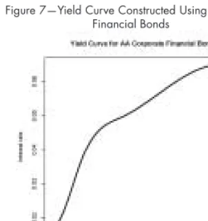
redemption yield on this index is 5.737 as of 3 March 2004. The last scenario is the corporate bond yield curve with AA-rated financial bonds again, but this time a constant spread of 50 basis points was subtracted as a risk adjustment. The 50 basis points are about the average spread reported in Table 1, and therefore the last scenario is a proxy for the Treasury yield curve.

In Table 13, we see that when using the corporate bond yield curve instead of the 30-year Treasury rate, liabilities increase by 0–3 % for older individ-uals and decrease up to 50% for younger individu-als. When using the corporate AA bond index, all liabilities would decrease, by 3–5% for older indi-viduals and up to 33% for younger indiindi-viduals. In the last scenario we changed Scenario 2 by subtract-ing a constant risk adjustment. Compared to the 30-year yield curve this leads to higher increases in liability for older people (3–6%) and lower decreas-es for younger people (up to 40%).

The reason for this behavior is that, for an upward sloping yield curve, the short end of the corporate bond yield curve can be lower than the 20-year Treasury rate. This will lead to higher values of short-term liabilities. This is offset by the higher yield on long-term corporate bonds, which leads to lower values for long-term liabilities. When

introducing the yield curve, pension plans with long-term liabilities will benefit more than those with short-term benefits, provided the yield curve is not inverted.

All in all, we see that in the current situation, exchanging the 30-year Treasury rate for a AA cor-porate bond index would lead to lower liabilities for pension funds. For a corporate bond yield curve, the situation is not that clear. Without a risk adjust-ment, increases would be quite small and only for a small group of people, but when using a risk adjust-ment, the increases would occur for all current retirees, while almost all people younger than 65 still working would have lower liabilities. The situ-ation of a specific pension fund depends then on the age structure of that fund.

Immunizing a pension fund against changes in the yield curve would require the fund to replicate the expected liabilities with their bond portfolio.8

However, with corporate bonds, which are defaultable, matching payouts or only matching the duration of the portfolio and the liabilities presents another problem. The effective duration of a corporate bond is shorter than its actual dura-tion because default can occur. The earlier payout of (part of ) the principal leads to a reduced dura-tion of the bond portfolio so that changing inter-est rates would affect the liabilities and the bond portfolio differently.

Some institutions have voiced concerns that using a corporate bond rate will decrease calculated pension liability values, therefore requiring less funding by the companies, and in effect eroding the financial basis of the pension system. However, when discussing whether liabilities will increase using the yield curve instead of the 30-year Treasury rate, it has to be noted that this very much depends on the exact yield curve used (type of bonds, risk adjustments) and the interest rate

8 _{Other sources of risk such as uncertainty in the amont of future payments (e.g., due to salary increases or inflation adjustments)}

or the time point of the future payouts (e.g., uncertainty about the time of retirement and death of the plan participants) remain. Figure 7—Yield Curve Constructed Using AA-Rated

environment. Both scenarios with an increase and a decrease in liabilities are possible. Overall, it can be said that the higher the risk adjustment and the better the quality of the bonds, the lower the resulting interest rates will be and thus the higher the liability values. Furthermore, as we compare a long-term rate against a yield curve, the behavior of the yield curve at the short end is important. If the interest rate at the short end is higher than the 30-year Treasury rate (in a scenario of a flat or inverted yield curve), liabilities would decrease. In the other case, liabilities would tend to increase.

All in all, the question whether liabilities will increase or decrease cannot be answered in a general sense at this point, and even after the exact yield curve methodology is known, both situations may occur. From this point of view the mentioned concerns of eroding the funding basis very well may be justified. However, valuing future payments using a yield curve approach (depending on risk adjustments) most accurately measures how much money has to be put into a portfolio of high-quality corporate bonds to be able to meet future obligations. Of course, using a lower rate increases liabilities and therefore improves funding. An in-depth study using various modeling approaches and interest rate scenar-ios should shed some light on the question of which actions are most appropriate to sustain of increase funding levels (low interest rates, higher required funding ratios, etc.). Unfortunately, conducting such a study is beyond the scope of this paper.

4.2 Discussion of Issues in Valuation of

Pension Plans

4.2.1 Interest-Sensitive Payment Forms

We now discuss the effect of valuation rates for cal-culating lump-sum payments and for the liabilities of an employee. The calculated liability reflects the amount of money set aside by the pension plan to fund the benefits of the employee. The use of a lower interest rate than the yield curve used in lia-bility calculations would increase the lump-sum payment. This would lead to increased payouts,

which would deplete the pension plan funds, mak-ing additional fundmak-ing necessary. Apart from this, it would be an incentive for retirees to take the lump sum instead of the annuity — increasing their per-sonal old-age funding risk. On the other hand, an interest rate that is higher than the yield curve would discriminate against those who choose the lump sum and reallocate pension money to the other pension plan participants. Therefore, when calculating lump-sum payments and valuing liabili-ties, it is important to use the same interest rates.

As the short end of the yield curve is more volatile than the long end, using the yield curve for lump-sum calculations will increase the volatility of the lump sum, making it harder for the employee to estimate what amount of money he or she can get upon retirement. This, however, just reflects the volatility in the plan assets (also in the case of bonds), which the pension plan has to face as well. Using a less volatile interest rate for these valuations would lead to the problems outlined above and in addition reallocate market risk to the other plan participants or the funding company.

To summarize, the only way to make the pension fund indifferent toward whether annuities or lump sums are paid is to compute lump sums using the liability discount rates. It should be noted that we have ignored mortality adverse selection in this discussion.

However, another issue has raised concerns among actuaries in the United States. New legis-lation contemplates requiring using today’s yield curve for calculating future lump-sum values instead of the estimated future yield curve. We will show the effects of these two possibilities with a short example. Assume an employee aged x today (t = 0) would currently get $1 per year upon retirement at the normal retirement age r. We want to value this liability using today’s yield curve.

We get

where the second equality holds because (T – t)

R(t,T) = (T1– t) R(t,T1) + (T – T1) R(t,T1,T),

which can be shown by a brief calculation. Here

Lr–xis the liability at t = r – x years, if the employ-ee is still living, and using the yield curve that the market expects in r – x years when the employee reaches retirement age (the appropriate forward rate curve), that is, the lump sum the employee could get upon retirement. We see that today’s liability L is the same as the liability in r – x years,

Lr–x, multiplied by the probability that the employee is still living r – x years from now and discounted using the r – x year spot rate. Therefore, the plan is indifferent between the annuity and the lump-sum payment. What hap-pens if we use today’s yield curve to compute the liability Lr–x instead of the appropriate forward rate? We then get

For an upward sloping yield curve, the liability when using today’s yield curve instead of the future rates would be higher and lower for downward slop-ing yield curves. Usslop-ing the yield curve from above, we get the changes in liability at time t = 0 shown in Table 14.

4.2.2 Cash Balance Plans

Cash balance plans have become more popular in recent years, so we want to discuss them a bit more closely. In a cash balance plan a fixed percentage of pay is credited on an account. Apart from this, interest on the account is also credited to the account. The interest rate can be a fixed rate, change from year to year, or be tied to an index. How is the actuarial liability affected by these choices? First, it is in general not equal to the account balance of the employee and in fact can vary very much, depend-ing on the chosen actuarial funddepend-ing method. Lowman (2000) showed in his study that the fund-ing method can change the actuarial liability of an employee up to 40% (at a certain age of the employee; other assumptions are omitted here). Of course, the interest rate for the plan also has a large impact. However, no general method exists for choosing the interest rate so that actuarial liability is close to the account balance for every plan partici-pant all the time. For simplicity, we will discuss this just for the traditional unit credit method. Other methods will require different solutions. In the case of the unit credit method, the account balance is projected to the normal retirement age using the plan's interest rate or an estimation in case it is still unknown. Then the resulting amount is discounted back using the spot rate curve. The case becomes

Table 14

Changes in Liability of Annuities if Using Spot Rate for Lump-Sum Valuation instead of Forward Rate (Retirement Age 65)

Age Forward Rate Spot Rate Change Spot-Forward

60 8.25 9.34 13.10%

50 3.89 4.67 20.24

40 1.94 2.14 10.62

30 1.01 1.12 10.62

20 0.53 0.58 10.62

∞

∞ ∞

THEPENSIONFORUM

particularly easy if the one-year spot rate of the curve is used as the account interest rate. The esti-mates for future interest rates would then be the appropriate forward rates, and the projection and discounting back would just set each other off. Of course, even then the actuarial liability still does not have to be equal to the account balance because of possible forfeitures (termination of employment before vesting, death). However, if the account bal-ance is paid as a lump sum in case of death before retirement, it should be close, as no leveraging has been anticipated. When a fixed interest rate is being used, this largely depends on the current interest rate environment. If the account interest rate is below the spot rate, leveraging will lead to an actu-arial liability that is below the account balance. Another related issue occurs in the case where the employee wants to have pension benefits in the form of a lump sum earlier than the scheduled retirement age. Depending on the interest credit rate, the account balance projected to retirement age and discounted back using the spot rate curve can be higher or lower than the account balance. IRS Notice 96-8 deals with the important ques-tion under which circumstances the plan has to pay more than the account balance to an employ-ee who receives a lump-sum payment. The mini-mum lump-sum computation rules of IRC Section 417(e) prescribe projecting the account balance to retirement age, converting it to an actuarially equivalent annuity, and discounting it back to the employment termination date using the 30-year Treasury rate. If this amount is greater than the account balance, the employee has to receive the higher amount. IRS Notice 96-8 also determines under which circumstances these cal-culations do not have to be performed. How these regulations change when a yield curve is used is

still unclear. More information on cash balance plans can be found in Lowman (2000), Coleman (1998), and Kopp and Sher (1998).

4.2.3 Embedded Options in Plan

Structure

Pension plans often include provisions for alterna-tive retirement ages, additional benefits for early retirees, or shutdown benefits. When using the yield curve, the valuation formulas have to be adjusted appropriately to reflect different interest rates for payments at different points in time. However, stating whether liabilities will increase or decrease is not possible for the reasons men-tioned above. Table 15 reports values of annuities for employees aged x, triggered at once, using the scenarios and assumptions mentioned above. The effect of changing from the Treasury rate against to the yield curve seems to have a significant impact, especially for young people. When using the yield curve with the risk adjustment, this effect is substantially reduced. However, without a detailed study, no firm statement can be made on the effects on embedded options of a change from a Treasury to a yield curve model.

4.2.4 Smoothing of the Yield Curve

Until now the discount rate used for measuring plan obligations has been a 4/3/2/1 weighted average, going back in time, of the Treasury rates of the last four years. This weighting is designed to reduce volatility in the market. It has been claimed (see, e.g., Ryan Labs, Inc. 2001) that no averaging should be used for valuation purposes. When hedging a risk such as future payments, one can transact only at market prices. Using weighted interest rates may lead to the situation that the actuarial liability and the cost for future

Table 15

Life Annuity Values, Payable at Different Ages for Varying Interest Rate Scenarios

Age x Scenario 1 Scenario 2 Scenario 3 Scenario 4 Change 2-1 Change 3-1 Change 4-1

40 17.57 15.87 15.90 16.83 -9.69% -9.49% -4.19%

50 15.89 14.78 14.58 15.57 -6.98 -8.25 -2.01

55 14.76 13.97 13.64 14.65 -5.34 -7.54 -0.69

payments on the market may deviate. Also, the reduction of volatility will depend on the partic-ular asset class or payment value under consider-ation. While the overall liability of a pension may be more volatile using a yield curve, the dif-ference between liabilities and asset values may (depending on the assets) become less volatile. For example, consider a fully funded pension plan with a portfolio of bonds that match future payments. Using an unsmoothed yield curve, the effect of changing interest rates is the same for the asset and the liability sides. When using smoothing, over- or underfunding can occur, although the portfolio still matches future pay-ments because the liability side is affected differ-ently than the asset side.

Another issue is the volatility of pension contribu-tions to meet newly acquired obligacontribu-tions. The volatility just reflects the underlying economic conditions. Another, more transparent, way of stabilizing contributions is to adapt the funding measures used.

Even if smoothing of the yield curve should be adopted, some issues remain unclear. Smoothing might result in “strange” shapes of the yield curve. This can be undesirable, as one gets unrealistic scenarios. Apart from this, the way smoothing should be done and especially in which sense this smoothing method would be optimal remain to be discussed.

5. Conclusion and Issues for Further

Research

The proposed termination of the 30-year Treasury bonds by the U.S. government make it necessary to consider different interest rate than the 30-year Treasury rate for pension valuation purposes. An investment-grade corporate bond yield curve measures today's market value of future payments quite accurately, the better the higher the rating of the bonds. The mathematical tools needed to extract the yield curve from market bond data are well developed and well tested. One issue when

THEPENSIONFORUM

References

Actuarial Standards Board. 1996. Actuarial

Standards of Practice No. 27: Selection of Economic Assumptions for Measuring Pension Obligations. Washington, D.C. December.

Actuarial Standards Board.

Anderson, Nicola, and John Sleath. 2001. New Estimates of the UK Real and Nominal Yield Curves. Working paper, Bank of England. Bader, Lawrence N. 1994. Introducing the

Salomon Brothers Pension Discount CurveSM

and the Salomon Brothers Pension Liability IndexSM_{: Discounting Pension Liabilities and}

Retiree Medical Liabilities under the New SEC Interpretation. March. Technical report, Salomon Brothers.

Bader, Lawrence N., and Y. Y. Ma. 1995. The Salomon Brothers Pension Discount CurveSM

and The Salomon Brothers Pension Liability IndexSM_{. Technical report, Salomon Brothers.}

Bekdache, Basma, and Christopher F. Baum. 1997. The Ex-Ante Predictive Accuracy of Alternative Models of the Term Structure of Interest Rates. Working paper, Boston College. Berndt, Antje. 2003. Estimating the Term Structure of Credit Spreads from Callable Corporate Bond Price Data. Working paper, Cornell University, Department of Operations Research and Industrial Engineering.

Bingham, N. H., and R. Kiesel. 2004.

Risk-Neutral Valuation. 2nd ed. Springer Finance.

Springer.

Bjork, T., and B. J. Christensen. 1997. Interest Rate Dynamics and Consistent Forward Rate Curves. Working paper, University of Aarhus. Blanco, Roberto, Simon Brennan, and Ian W.

Marsh. 2003. An Empirical Analysis of the Dynamic Relationship between Investment Grade Bonds and Credit Default Swaps. Working paper, Bank of England.

Bliss, Robert R. 1996. Testing Term Structure Estimation Methods. Working paper, Federal Reserve Bank of Atlanta.

Bolder, David Jamieson, and Scott Gusba. 2002. Exponential, polynomials, and Fourier Series:

More Yield Curve Modelling at the Bank of Canada. Working paper, Bank of Canada. Coleman, Dennis. 1998. The Cash-Balance

Pension Plan. Pension Forum, October. Collin-Dufresne, Pierre, Robert S. Goldstein, and

J. Spencer Martin. 2001. The Determinants of Credit Spread Changes. Journal of Finance 56(6): 2177-2207.

Dahlquist, Magnus, and Lars E. O. Svensson. 1996. Estimating the Term Structure of Interest Rates for Monetary Policy Analysis.

Scandinavian Journal of Economics 98(2):

163-183.

Delianedis, Gordon, and Robert Geske. 2001. The Components of Corporate Credit Spreads: Default, Recovery, Tax, Jumps, Liquidity and Market Factors. Working paper, University of California, Los Angeles.

Diaz, Antonia, and Frank S. Skinner. 2001. Estimating Corporate Yield Curves. Journal of

Fixed Income 11(2): 95-103.

Duffee, Gregory R. 1996. Treasury Yields and Corporate Bond Yield Spread: An Empirical Analysis. Working paper, Federal Reserve Board.

———1998. The Relation Between Treasury Yields and Corporate Bond Yield Spreads.

Journal of Finance 53(6): 2225-41.

Düllmann, Klaus, Marliese Uhrig-Homburg, and Marc Windfuhr. 1998. Risk Structure of Interest Rates: An Empirical Analysis for Deutschemark-Denominated Bonds. Working paper, University of Mannheim.

Elton, Edwin J., Martin J. Gruber, Deepak Agrawal, and Christopher Mann. 2001. Explaining the Rate Spread on Corporate Bonds. Journal of Finance 56(1): 247-77. Fama, E. F., and K. R. French. 1993. Common

Risk Factors in the Return on Stocks and Bonds. Journal of Financial Economics 33: 3-56. Fama, E. F., and R. R. Bliss. 1987. The Information in Long-Maturity Forward Rates.

American Economic Review 77 (September):