www.biogeosciences.net/11/2939/2014/ doi:10.5194/bg-11-2939-2014
© Author(s) 2014. CC Attribution 3.0 License.
Examination of the role of the microbial loop in regulating lake
nutrient stoichiometry and phytoplankton dynamics
Y. Li1,2,3, G. Gal4, V. Makler-Pick5,6, A. M. Waite7,*, L. C. Bruce1,7, and M. R. Hipsey1,7
1Aquatic Ecodynamics, School of Earth & Environment, The University of Western Australia, Crawley WA 6009, Australia 2Department of Ecology, Jinan University, Guangzhou 510632, China
3School of Environmental Science & Engineering, Ocean University of China, Qingdao 266100, China. 4Kinneret Limnological Laboratory, Israel Oceanographic and Limnological Research, Migdal 14950, Israel 5Faculty of Civil and Environmental Engineering, Technion-Israel Institute of Technology, Haifa 32000, Israel 6Oranim Academic College of Education, Kiryat Tivon 36006, Israel
7The Oceans Institute, The University of Western Australia, Crawley WA 6009, Australia
*current address: Alfred-Wegener-Institut Helmholtz-Zentrum für Polar- und Meeresforschung, Am Handelshafen 12, 27570
Bremerhaven, Germany
Correspondence to: M. R. Hipsey ([email protected])
Received: 8 July 2013 – Published in Biogeosciences Discuss.: 16 December 2013 Revised: 3 May 2014 – Accepted: 6 May 2014 – Published: 5 June 2014
Abstract. The recycling of organic material through bacteria and microzooplankton to higher trophic levels, known as the “microbial loop”, is an important process in aquatic ecosys-tems. Here the significance of the microbial loop in influenc-ing nutrient supply to phytoplankton has been investigated in Lake Kinneret (Israel) using a coupled hydrodynamic– ecosystem model. The model was designed to simulate the dynamic cycling of carbon, nitrogen and phosphorus through bacteria, phytoplankton and zooplankton functional groups, with each pool having unique C : N : P dynamics. Three mi-crobial loop sub-model configurations were used to isolate mechanisms by which the microbial loop could influence phytoplankton biomass, considering (i) the role of bacterial mineralisation, (ii) the effect of micrograzer excretion, and (iii) bacterial ability to compete for dissolved inorganic nu-trients. The nutrient flux pathways between the abiotic pools and biotic groups and the patterns of biomass and nutrient limitation of the different phytoplankton groups were quan-tified for the different model configurations. Considerable variation in phytoplankton biomass and dissolved organic matter demonstrated the sensitivity of predictions to assump-tions about microbial loop operation and the specific mech-anisms by which phytoplankton growth was affected. Com-parison of the simulations identified that the microbial loop most significantly altered phytoplankton growth by
periodi-cally amplifying internal phosphorus limitation due to bacte-rial competition for phosphate to satisfy their own stoichio-metric requirements. Importantly, each configuration led to a unique prediction of the overall community composition, and we conclude that the microbial loop plays an important role in nutrient recycling by regulating not only the quan-tity, but also the stoichiometry of available N and P that is available to primary producers. The results demonstrate how commonly employed simplifying assumptions about model structure can lead to large uncertainty in phytoplankton com-munity predictions and highlight the need for aquatic ecosys-tem models to carefully resolve the variable stoichiometry dynamics of microbial interactions.
1 Introduction
paradigm, which assumes a relatively simple flow of nutri-ents to autotrophic and then heterotrophic pools. However, it is now well-documented both in oceanographic and, to a lesser extent, in limnological applications, that higher order predators such as crustacean zooplankton or fish can be sup-ported by two paths: the so-called “green” (algal-based) and “brown” (detrital-based) food web components (Moore et al., 2004). The latter refers to the dynamics of the heterotrophic bacteria and the microzooplankton grazers (defined here as size less than 125 µm that account for rotifers, ciliates and juvenile macrograzers; Thatcher et al., 1993) – often termed the “microbial loop”. This has been shown to play an im-portant role in shaping carbon fluxes in lakes and in enhanc-ing nutrient cyclenhanc-ing at the base of food webs (Gaedke et al., 2002), including in Lake Kinneret which is the focus in this study (Stone et al., 1993; Hart et al., 2000; Hambright et al., 2007; Berman et al., 2010).
Less well understood is how the microbial loop affects phytoplankton growth and thus potentially shape patterns of phytoplankton succession. There are several main mecha-nisms by which microbial loop processes are thought to in-fluence phytoplankton dynamics: (i) the provision of bacteri-ally mineralised nutrients for phytoplankton growth; (ii) the excretion of readily available nutrients by micrograzers that support primary production (Johannes, 1965; Wang et al., 2009); (iii) the competition of bacteria with phytoplankton for inorganic nutrients when organic detritus becomes nutri-ent depleted (Barsdate et al., 1974; Bratbak and Thingstad, 1985; Stone, 1990; Kirchman, 1994; Caron, 1994; Joint et al., 2002; Danger et al., 2007). Additionally, a potential fourth indirect mechanism is that bacteria provide an alternative food source for micrograzers, thus alleviating some grazing pressure from small primary producers. The relative signif-icance of each of these mechanisms, and in particular how they interact in a dynamic environment to shape microbial community composition and influence net productivity re-mains unclear.
Models of lake ecosystems are increasingly common to support management and analysis of water quality prob-lems, acting as ‘virtual’ laboratories for exploring ecosystem processes particularly for questions where empirical studies would be difficult to undertake (Van Nes and Scheffer, 2005; Mooij et al., 2010). In most models published to date it is generally assumed that the biomass of heterotrophic bacteria is fairly stable and that the majority of bacterial production is lost to respiration (Cole, 1999). As a result, most quan-titative models of carbon and nutrient fluxes in freshwater ecosystems essentially simplify microbial loop processes by assuming a relatively static mineralisation rate of organic ma-terial and simulating direct zooplankton consumption of de-tritus as a proxy for microzooplankton consumption of bac-teria (e.g. Janse et al., 1992; Saito et al., 2001; Bruce et al., 2006; Mooij et al., 2010). These simplifications do not cap-ture the range of nutrient ‘adjustments’ that occur during mi-crobial loop processes, since stoichiometric composition of
organisms and the fluxes between them are in reality neither uniform nor static (Elser and Urabe, 1999; Sterner and Elser, 2002). Whilst representation of microbial loop processes has been developed in marine ecosystem models (e.g. Faure et al., 2010), their uptake in freshwater ecosystem models has been limited and none to our knowledge simultaneously re-solve the microbial loop and the dynamic stoichiometry of carbon (C), nitrogen (N) and phosphorus (P).
As a background to this study, there have been several attempts to incorporate the microbial loop into Lake Kin-neret ecosystem models. Initially, a steady-state C flux model was developed to examine C cycling through the plank-tonic biota, including consideration of the microbial loop (Stone et al., 1993; Hart et al., 2000). A one-dimensional (1-D) coupled hydrodynamic–ecosystem model (DYRESM-CAEDYM) was presented by Bruce et al. (2006), which fo-cused specifically on the zooplankton dynamics and their contribution to nutrient recycling. However, the model pre-sented by Bruce et al. (2006) had a simplistic representation of the microbial loop dynamics, like many contemporary lake ecosystem models, and also did not individually simulate two important cyanobacterial species, Microcystis sp. and
Aph-anizomenon sp., which are important to the health of the
ecosystem and sensitive to stoichiometric constraints within the food web (Zohary, 2004). Gal et al. (2009) expanded this model to include a dynamic microbial loop parameterisation and accounted for the two cyanobacterial species listed above and validated the model approach against a comprehensive data set. The relationship between phytoplankton stoichiom-etry and patterns in the stoichiomstoichiom-etry of available nutrients was further analysed by Li et al. (2013), who noted that the microbial loop parameterisation approach could adjust both the quantity and stoichiometry of nutrient transfers.
This research builds on these studies and applies the val-idated model with the general aim of isolating the signifi-cance of the microbial loop on the phytoplankton patterns within the lake. Specifically, three different microbial loop model structural configurations were designed and analysed to unravel how the microbial loop processes identified above combine to affect (a) the stoichiometry of nutrient trans-fers through the planktonic food web, and (b) phytoplank-ton growth and community composition. The results high-light the importance of resolving the variable stoichiometry of microbial interactions in aquatic models and suggest that commonly used simplifying assumptions may compromise model function.
2 Method
2.1 Site description
has a maximum depth of 43 m, and has been the focus of con-siderable limnological research over the past few decades. Major phytoplankton groups present in the lake include
Peri-dinium sp., Aulacoseira sp., Aphanizomenon sp., Microcys-tis sp. and nanophytoplankton. A number of zooplankton
species occur in the lake and can be grouped as rotifers, ciliates, and herbivorous (cladocerans and copepodites) and predatory zooplankton (adult copepods). The maximum cil-iate abundance is observed in autumn, generally preceding a metazooplankton peak. Heterotrophic nanoflagellates are most abundant in winter and spring, and least abundant in autumn. Bacteria numbers are highest during the decline of the Peridinium gatunense (hereafter referred to as
Peri-dinium) bloom and are the lowest during the winter (Hadas
et al., 1998). Lake Kinneret was once well known for sea-sonal blooms of Peridinium that regularly occurred until the late 1990s (Zohary et al., 1998; Zohary, 2004; Roelke et al., 2007). However, observations over the last decade have seen a major decline in Peridinium and a disruption in the histor-ically stable patterns of phytoplankton succession (Zohary, 2004). In response, the biomass of Aulacoseira blooms has changed and the contribution of cyanobacteria and nanophy-toplankton to the total phynanophy-toplankton biomass has increased in summer. Due to reduced water quality, the occurrence of nuisance cyanobacterial blooms is an increasing concern (Ballot et al., 2011).
2.2 Model overview and simulation approach
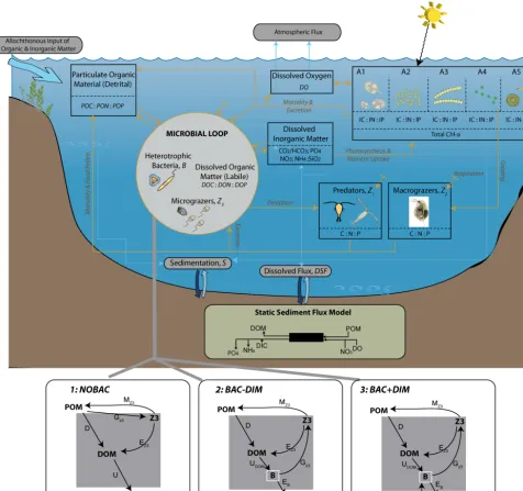
In this study, the 1-D hydrodynamic–ecological model DYRESM-CAEDYM was applied to the lake for the pe-riod from 1997 to 2001. The configuration adopted here is a continuation from Gal et al. (2009), with three microbial loop sub-model configurations applied (Fig. 1), as described below. The model simulates phytoplankton dynamics, bac-terial production, carbon and nutrient recycling, sediment– water interactions, and relevant inflow, outflow and mixing processes. In each simulation conducted, five phytoplankton groups, A, are included, each with three state variables (in-ternal C, N, and P, denoted asA, AIN, and AIP, respectively):
Peridinium (A1), Microcystis (A2), Aphanizomenon (A3),
nanophytoplankton (A4) and Aulacoseira (A5). Three
zoo-plankton functional groups, Z, each with fixed internal nu-trient ratios, were also simulated: predatory copepods (Z1),
macrograzers (Z2) and microzooplankton (Z3). Bacteria (B)
were modelled as a separate state variable for two of the mi-crobial loop configurations. An additional 10 nutrient vari-ables (FRP, NO3, NH4, DIC, DOC, DON, DOP, POC, PON,
POP), and dissolved oxygen (DO) were also modelled, giv-ing a total of 30 biogeochemical state variables (Table 1). Field data was used to initialise the vertical profiles of all major state variables.
Earlier versions of the model (Gal et al., 2009, Makler-Pick et al., 2011a, b; Li et al., 2013) have been thoroughly validated against field data and process measurements
(Ap-pendix A). Here we use the best-calibrated model version from these studies to explore the impact of changes in bac-terial dynamics on patterns of phytoplankton growth. Within a well-documented set of core ecological process parameters determined elsewhere, we vary the structure and function of the microbial loop to assess how these changes would impact broader ecosystem biogeochemistry. Therefore, while this is essentially a theoretical study, it remains nested in a robust modelling framework built on a strong process understand-ing of the Lake Kinneret ecosystem.
2.3 Bacteria and microbial loop sub-models
Three alternative microbial loop sub-model configurations were compared to evaluate the relative importance of the three key mechanisms by which the microbial loop can affect phytoplankton dynamics (Table 2). Note that in this study we are not further considering the role of the fourth indirect mechanism listed in the introduction, since in Lake Kinneret the micrograzer food source is thought to be predominantly bacteria. The three simulations are differentiated by having (1) an assumed constant bacteria biomass state variable us-ing static organic matter mineralisation rates and microzoo-plankton grazing directly on POM (NOBAC hereafter); (2) bacteria simulated with dynamic biomass and hence miner-alisation rates, but unable to take up dissolved inorganic N and P (BAC−DIM hereafter); (3) dynamic bacteria (as per 2) with an additional ability for supplementing their internal nutrient requirement with dissolved inorganic N and P (PO4
and NO3/ NH4) if the available organic matter becomes
nu-trient deplete (BAC + DIM hereafter).
The general mathematical description of the mass balance for each of the variables and associated notations are in Ta-ble 3. For each configuration, parameterisation of the com-mon microbial loop process pathways are described in de-tail next and summarised in Table 4. For other CAEDYM variable descriptions, process equations and parameter val-ues and justifications, readers are referred to Gal et al. (2009). 2.3.1 Common processes in all configurations
POM hydrolysis
This process considers the enzymatic hydrolysis and decom-position (DPOM) of particulate detrital material, limited by
dissolved oxygen concentration (DO) and bacterial biomass (B) if bacteria are simulated:
D=µPOM maxfBT(T )min h
fBDOB(DO)fB(B)
i
POM, (1) whereµPOM maxis the maximum transfer of POM to DOM,
and refers to one ofµPOC max,µPON max, orµPOP max
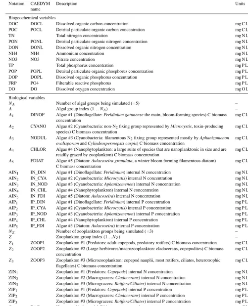
Table 1. Overview of model variables indicating CAEDYM state variable name where relevant.
Notation CAEDYM Description Units
name
Biogeochemical variables
DOC DOCL Dissolved organic carbon concentration mg C L−1
POC POCL Detrital particulate organic carbon concentration mg C L−1
TN Total nitrogen concentration mg N L−1
PON PONL Detrital particulate organic nitrogen concentration mg N L−1
DON DONL Dissolved organic nitrogen concentration mg N L−1
NH4 NH4 Ammonium concentration mg N L−1
NO3 NO3 Nitrate concentration mg N L−1
TP Total phosphorus concentration mg P L−1
POP POPL Detrital particulate organic phosphorus concentration mg P L−1
DOP DOPL Dissolved organic phosphorus concentration mg P L−1
FRP PO4 Filterable reactive phosphorus mg P L−1
DO DO Dissolved oxygen concentration mg O L−1
Biological variables
NA Number of algal groups being simulated (= 5) –
A Algal group index (1. . .NA) –
A1 DINOF Algae #1 (Dinoflagellate: Peridinium gatunense the main, bloom-forming species) C biomass
concentration
mg C L−1
A2 CYANO Algae #2 (Cyanobacteria: non-N2fixing group represented by Microcystis, toxin-producing
species) C biomass concentration
mg C L−1
A3 NODUL Algae #3 (Cyanobacteria: filamentous N2fixing group represented mostly by Aphanizomenon
ovalisporum and Cylindrospermopsis cuspis) C biomass concentration
mg C L−1
A4 CHLOR Algae #4 (Nanophytoplankton: a large suite of species that are nanoplanktonic in size and are
readily grazed by zooplankton) C biomass concentration
mg C L−1
A5 FDIAT Algae #5 (Diatom: Aulacoseira granulata, a winter bloom forming filamentous diatom)
C biomass concentration
mg C L−1
AIN1 IN_DIN Algae #1 (Dinoflagellate: Peridinium) internal N concentration mg N L−1
AIN2 IN_CYA Algae #2 (Cyanobacteria: Microcystis) internal N concentration mg N L−1
AIN3 IN_NOD Algae #3 (Cyanobacteria: Aphanizomenon) internal N concentration mg N L−1
AIN4 IN_CHL Algae #4 (Nanophytoplankton) internal N concentration mg N L−1
AIN5 IN_FDI Algae #5 (Diatom: Aulacoseira) internal N concentration mg N L−1
AIP1 IP_DIN Algae #1 (Dinoflagellate: Peridinium) internal P concentration mg P L−1
AIP2 IP_CYA Algae #2 (Cyanobacteria: Microcystis) internal P concentration mg P L−1
AIP3 IP_NOD Algae #3 (Cyanobacteria: Aphanizomenon) internal P concentration mg P L−1
AIP4 IP_CHL Algae #4 (Nanophytoplankton) internal P concentration mg P L−1
AIP5 IP_FDI Algae #5 (Diatom: Aulacoseira) internal P concentration mg P L−1
NZ Number of zooplankton groups being simulated ( =3) –
Z Zooplankton group index (1. . .NZ) –
Z1 ZOOP1 Zooplankton #1 (Predators: adult copepods, predatory rotifers) C biomass concentration mg C L−1
Z2 ZOOP2 Zooplankton #2 (Large herbivores/macrozooplankton: cladocerans, copepodites) C biomass
concentration
mg C L−1
Z3 ZOOP3 Zooplankton #3 (Microzooplankton: copepod nauplii, most rotifers, ciliates, heterotrophic
flagellates) C biomass concentration
mg C L−1
ZIN1 Zooplankton #1 (Predators: Copepods) internal N concentration mg N L−1
ZIN2 Zooplankton #2 (Macrograzers: Cladocerans) internal N concentration mg N L−1
ZIN3 Zooplankton #3 (Micrograzers: Rotifers/Ciliates) internal N concentration mg N L−1
ZIP1 Zooplankton #1 (Predators: Copepods) internal P concentration mg P L−1
ZIP2 Zooplankton #2 (Macrograzers: Cladocerans) internal P concentration mg P L−1
ZIP3 Zooplankton #3 (Micrograzers: Rotifers/Ciliates) internal P concentration mg P L−1
B BAC Heterotrophic bacterial C biomass concentration mg C L−1
BIN Heterotrophic bacterial internal nitrogen concentration mg N L−1
Figure 1. Conceptual diagram highlighting the general ecosystem model (CAEDYM) configuration for Lake Kinneret (top) and processes
and feedbacks for the three microbial loop models (bottom) explored in this study: (1) NOBAC, (2) BAC−DIM, and (3) BAC + DIM (refer
to Tables 1 and 3 for notation).
DOM mineralisation
Whilst the mineralisation of DOM to DIM is common to all configurations, when the bacteria state variable is included the process adopts a two-stage breakdown pathway as shown in the subsequent details of the BAC−DIM and BAC + DIM configurations. The general rate of DOM breakdown/uptake (UDOC) is simulated as
UDOC= (2)
µDOC maxfBT(T )fBDOB(DO)DOC
NOBAC
µDECDOMfBT(T )minfBDOB(DO)fB(B)DOC BAC−DIM and BAC+DIM,
whereµDECDOMis the maximum bacterial DOM uptake rate
Table 2. Summary of three microbial loop simulations configured.
Model description NOBAC BAC−DIM BAC + DIM
Phytoplankton: A1–5 A1–5 A1–5
Zooplankton: Z1–3 Z1–3 Z1–3
Bacteria: 0 1 1
Microzooplankton grazing
Assumes bacteria com-bined in detritus pool, which is grazed by mi-crozooplankton
Assumes a dynamic heterotrophic bacterial pool that is grazed upon by microzooplankton, including C, N and P transfer
Assumes a dynamic heterotrophic bacte-rial pool that is grazed upon by microzoo-plankton, including C, N and P transfer
Organic matter breakdown
Occurs at a constant rate, and C, N and P are broken down in a con-stant proportion
DOM consumption linked to bacte-rial biomass. Rate of mineralisation and bacterial biomass growth slows if bacteria can not satisfy N or P re-quirement from the DOM pool.
DOM consumption linked to bacte-rial biomass. Rate of mineralisation not linked to DOM stoichiometry and
bacte-ria consume NO3or PO4if they cannot
satisfy N or P requirement from the DOM pool.
Mechanisms by which microbial loop impacts phytoplankton
(i) bacterial mineralisa-tion of nutrients
(i) bacterial mineralisation of nutri-ents
(ii) micrograzers respond to vari-able bacteria concentration and ex-crete labile DOM rich in N and P
(i) bacterial mineralisation of nutrients (ii) micrograzers respond to variable bac-teria concentration and excrete labile DOM rich in N and P
(iii) bacteria compete for inorganic nutri-ents
Comment Typical of most lake
eutrophication models that do not include bac-teria
Used in model studies where bac-teria are simulated but stoichiome-try is not specifically a constraint on bacterial production
Most likely the closest representation to reality with bacteria biomass variable and inorganic nutrient uptake used to support bacterial growth requirement
Micrograzer grazing
All simulations include microzooplankton (Z3), which graze
either on a lumped detrital pool (NOBAC) or directly on bac-teria (BAC−DIM and BAC + DIM). For simplicity, micro-zooplankton are considered to graze on either bacteria or de-tritus, since the rate of grazing on small size phytoplankton (A4) has been reported to be relatively low compared to the
rate of bacterial grazing (∼10 % of total microzooplankton diet in Lake Kinneret; Hambright et al., 2007).
Micrograzer excretion and respiration
In all configurations micrograzers respire (R) and excrete (E) labile organic matter:
RZ3=kZrfZT32(T ) Z3 (3)
EDOC=(1−kmf) kZeGC(Z3), (4)
wherekZris the respiration rate andkZeis the DOC
excre-tion rate. Since micrograzers are configured to have a stable C:N:P requirement, their excretion of N and P is variable in order to balance the other output nutrient fluxes. This is nu-merically achieved by performing the excretion at the end of
the time step after other terms have been accounted for:
EDON=
ZIN∗3−Z3t+1kZIN3
1t (5)
where ZIN∗3=ZINt3+GZ3(BIN)−EDON−MZ3−PZ1
EDOP=
ZIP∗3−Z3t+1kZIP3
1t (6)
where ZIP∗3=ZIPt3+GZ3(BIP)−EDOP−MZ3−PZ1,
wherekZIN is the internal ratio of N to C and kZIP is the
internal ratio of P to C of the particular zooplankton class. 2.3.2 Configuration 1 – NOBAC
This configuration assumes organic matter is mineralised at a rate that is not dependent on the bacterial biomass (i.e. the bacterial biomass is assumed non-limiting and fB(B) in Eq. (1) is fixed at 1). This approach moves C, N and P fluxes between DOM and DIM proportionally. Since there are no bacteria simulated for micrograzers to graze upon, the grazing preferences were adjusted to consume POM in place of bacteria, thereby assuming bacterial biomass is lumped within the detrital pool. The grazing rate of microzooplank-ton simplifies to
GZ3(POC)=gMAX
POC KZ3+POC
where POC is used to determine the grazing rate and PON and POP are consumed at a rate commensurate with their lo-cal stoichiometry at the time of grazing. The grazing rate pa-rameter (gMAX) was adjusted to makeGZ3(POC) in NOBAC
approximately equal toGZ3(B)in BAC + DIM (Table 4), to
keep the general C flow and biomass patterns comparable be-tween these simulations.
2.3.3 Configuration 2 – BAC−DIM
This configuration includes the heterotrophic bacteria state variable,B, however, they are restricted to DOM uptake dur-ing the mineralisation process. Under this scenario, the bac-terial biomass and their mineralisation rate increase and de-crease depending on temperature and organic matter avail-ability, but their nutrient requirement must be satisfied from the DOM pool. The basic equations for BAC−DIM are sim-ilar to NOBAC, except the inclusion of the bacterial equa-tion and their associated growth and loss processes (Table 3). Bacterial uptake of DOC is similarly defined using Eq. (2) withfB(B)defined as
fB(B)= B KB+B
. (8)
Bacterial uptake of DON and DOP is based on the C min-eralisation rate, converted according to the stoichiometric re-quirement of N and P (kBINandkBIP), but limited to the
avail-able pool to enforce mass conservation:
UDON= (
UDOC·kBIN DON> UDOC·kBIN1t
DON DON≤UDOC·kBIN1t
(9)
UDOP= (
UDOC·kBIP DOP> UDOC·kBIP1t
DOP DOP≤UDOC·kBIP1t .
(10) Note that if they cannot support the stoichiometric require-ment in line with the UDOC from the DON and DOP pool,
then they take what is available andUDOCwill be reduced
ac-cordingly. In this configuration, POM decomposition is also dependent on the changing bacterial biomass throughfB(B) and micrograzers graze on bacteria (B) rather than POM. ThereforeGZ3(B)is set as
GZ3(B)=gMAX
B KZ3+B
Z3. (11)
2.3.4 Configuration 3 – BAC + DIM
This configuration is an extension of BAC−DIM where bac-teria compete with phytoplankton by supplementing their in-ternal nutrient requirements through the uptake of inorganic nutrients when there is insufficient N and P in the DOM pool to support growth. The bacterial uptake of N and P requires the following additional terms (Table 3):
UNH4=
NH4 UDOC·kBIN1t >DON UDOC·kBIN−UDON UDON< UDOC·kBIN1t
0 UDON=UDOC·kBIN1t
(12)
UNO3=
NO3 UDOC·kBIN1t > DON+NH4
UDOC·kBIN−UDON−UNH4 UDON+UNH4< UDOC·kBIN1t
0 UDON+UNH4=UDOC·kBIN1t
(13)
UFRP=
UDOC·kBIP−UDOP UDOP< UDOC·kBIP1t
0 UDOP=UDOC·kBIP1t .
(14) If there is insufficient organic and inorganic N or P to support the carbon uptake rate,UDOC, the growth is limited to enforce
mass balance as in configuration 2. 2.4 Analysis procedure
2.4.1 Model sensitivity Structural sensitivity
The averages of a number of variables from the upper 10 m of the water column were computed over the simulated pe-riod (1997–2001) to be consistent with Gal et al. (2009). The physical (T, DO), chemical (TN, TP, NO3, NH4,
PO4) and biological variables (A1–5,Z1–3) of the NOBAC,
BAC−DIM, and BAC + DIM were statistically compared by one-way ANOVA (5 % significance level, SPSS software version 18.0) and Multiple Comparisons (POST HOC, SPSS software version 18.0) to determine significant differences between the outputs of the alternative microbial loop sub-models. Since model time series are not suited to ANOVA, our approach was to conduct monthly averages of surface layer model output to match the frequency of observational data that was used for validation. Given that the timescale for many processes is the order of days to weeks (e.g. Recknagel et al., 2013), this was done to reduce the degree of temporal auto-correlation between consecutive model points.
Parameter sensitivity
In addition, a sensitivity analysis of the impact of the mi-crobial loop parameters on the simulated C, N and P cycles for BAC + DIM was conducted, since this configuration was considered to be the most similar to the actual dynamics of the lake. The limited selection of parameters were chosen based on the detailed global analysis of the complete set of ecological parameters by Makler-Pick et al. (2011a), and rel-evance to the microbial loop processes investigated here. A simple “one-at-a-time” sensitivity analysis was undertaken by scaling the parameters individually by +20 % and−20 %, similar to Bruce et al. (2006), and the degree of sensitivity of state variable concentrations and major process pathways for C, N and P cycles were compared.
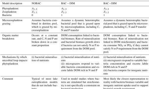
Table 4. Microbial-loop related parameters used in the three model simulations (refer to Gal et al. (2009) for other parameter values).
Parameter Units Description NOBAC BAC−DIM BAC + DIM Comments/other literature/justification
µPOCmax d−1 Maximum transfer of POC→DOC 0.07 0.07 0.07 Gal et al. (2009) values adopted. 0.001(1)
µPONmax d−1 Maximum transfer of PON→DON 0.01 0.01 0.01 0.02(1); 0.01-0.03(2)
µPOPmax d−1 Maximum transfer of POP→DOP 0.1 0.1 0.1 0.01(1); 0.01–0.1(2)
dPOM m Diameter of POM particles 5.50×10⁻⁶ 5.50×10⁻⁶ 5.50×10⁻⁶ Gal et al. (2009) values adopted; 1.50×10⁻⁵(1)
ρPOM kg m−3 Density of POM particles 1040 1040 1040 Gal et al. (2009) values adopted; 1.08×10³(1)
DOM parameters
µDOCmax d−1 Max mineralisation of DOC→DIC 0.0008 N/A N/A Estimated from average output from
BAC + DIM
µDOPmax d−1 Max mineralisation of DOP→PO4 0.1 N/A N/A 0.01(1); 0.01–0.1(2)
µDONmax d−1 Max mineralisation of DON→NH4 0.008 N/A N/A calibrated values adopted; 0.02(1); 0.01–0.03(2)
Bacteria parameters
vB Arrhenius temperature scaling factor 1.08 1.08 1.08 Gal et al. (2009) values adopted.
TSTDB ◦C Standard temperature 20 20 20 Gal et al. (2009) values adopted.
TOPTB ◦C Optimum temperature 30 30 30 Gal et al. (2009) values adopted.
TMAXB ◦C Maximum temperature 38 38 38 Gal et al. (2009) values adopted.
KDOB mg O2L−1 Half-saturation constant for dependence of
POM/DOM decomposition on DO
1.5 1.5 1.5 Gal et al. (2009) values adopted.
fAnB – Aerobic/anaerobic factor 0.8 0.8 0.8 Gal et al. (2009) values adopted.
kBr d−1 Bacterial respiration rate at 20◦C N/A 0.12 0.12 Gal et al. (2009) values adopted.
µDECDOC d−1 Maximum bacterial DOC uptake rate N/A 0.05 0.05 Gal et al. (2009) values adopted.
KB mg C L−1 Half-saturation constant for bacteria function N/A 0.01 0.01 Gal et al. (2009) values adopted.
KBIN mg N (mg C)−1 Internal C : N ratio of bacteria N/A 0.13 0.13 Gal et al. (2009) values adopted.
KBIP mg P (mg C)−1 Internal C : P ratio of bacteria N/A 0.0575 0.0575 Gal et al. (2009) values adopted.
KBe – DOC excretion N/A 0.7 0.7 Gal et al. (2009) values adopted.
µDIMupt DIM uptake Off Off On
Micrograzer (Z3) parameters
KZIN mg N (mg C)−1 Internal ratio of nitrogen to carbon 0.2 0.2 0.2 0.2(1); 0.24–0.27(3)
KZIP mg P (mg C)−1 Internal ratio of phosphorus to carbon 0.016 0.016 0.016 0.01(1); 0.016–0.43(3)
Pzp – Preference of zooplankton for POC 1 0 0 Pzp= 1 in NOBAC as no bacteria present; 1(1); 0.75(4)
Pzb – Preference of zooplankton for bacteria 0 1 1 Z3assumed to only graze on bacteria
gMAX mg C L−1 Grazing rate 9 9 9 Gal et al. (2009) values adopted;
(mg Z L−1)−1d−1
Kmf – Messy feeding (grazing efficiency) 0.75 0.75 0.75 Gal et al. (2009) values adopted; 1(1)
KZe d−1 Excretion fraction of grazing 0.25 0.25 0.25 Gal et al. (2009) values adopted; 0.2(1)
KZ mg C L−1 Half-saturation constant for grazing 0.4 1.5 1.5 0.5(1)(5); 0.1(5); 1.64(6) MINPOC mg C L−1 Minimum grazing limit for POC 0.075 N/A N/A Assumed
MINBAC mg C L−1 Minimum grazing limit for bacteria N/A 0.05 0.05 Gal et al. (2009) values adopted.
TSTDZ ◦C Standard temperature 20 20 20 Gal et al. (2009) values adopted.
TOPTZ ◦C Optimum temperature 24 24 24 Gal et al. (2009) values adopted.
TMAXZ ◦C Maximum temperature 30 30 30 Gal et al. (2009) values adopted.
(1)Bruce et al. (2006);
(2)Jorgensen and Bendoricchio (2001); (3)Martin et al. (2005);
(4)Gophen and Azoulay (2002); (5)Makler-Pick et al. (2011b); (6)Stemberger and Gilbert (1985).
averaged over the simulation period, with both nutrient and biological state variables and fluxes being vertically inte-grated to provide lake-wide averages.
For each of the phytoplankton groups, the nutrient limita-tion funclimita-tions,fa(N) andfa(P), at a depth of 1 m below the water surface were assessed to explore the impact of the mi-crobial loop on phytoplankton nutrient limitation. The func-tions were calculated by the model based on the internal nu-trient concentrations (Li et al., 2013):
fa(N)=
INMAXa
INMAXa−INMINa
1−INMINa
AINa
(15)
fa(P)=
IPMAXa
IPMAXa−IPMINa
1−IPMINa
AIPa
(16)
which range from 0 (extreme limitation) to 1 (no limitation).
3 Results
3.1 Comparison of model simulations
As expected, the simulated temperature and dissolved oxy-gen patterns were similar in the three models and matched the field data equally well (Appendix A). The simulated ma-jor nutrient results (TN, TP, NO3, NH4 and PO4) for the
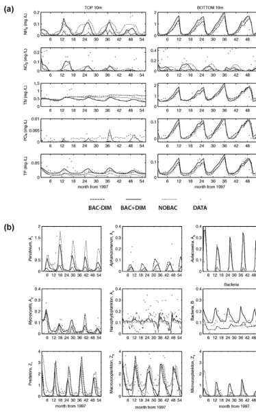
Figure 2. Comparison of model simulations for (a) nutrient variables in the surface 10 m (left) and the bottom 10 m (right) of the water
column (mg L−1), and (b) for the nine simulated biotic groups (mg C L−1forA1–5andB, and mg C m−2forZ1–3). Data represents the
PO4spikes in the simulated output of BAC−DIM, relative
to BAC + DIM. Also, relative to BAC + DIM, increased lev-els of TN were simulated in NOBAC and BAC−DIM. In terms of the microbes, all three configurations followed sim-ilar seasonal trends, however, noticeable differences were reduced bacteria and Peridinium and increased
Aphani-zomenon concentrations in BAC−DIM (Fig. 2b).
The impact of the three alternative microbial loop config-urations on the 15 physical, chemical and biological vari-ables was statistically analysed by one-way ANOVA and Multiple Comparisons (Table 5). Although the simulated results for T and DO were not significantly different in the three configurations, the simulated results for nutrients were significantly different (p <0.05): NH4, TN and TP of
BAC + DIM were significantly different from BAC−DIM and NOBAC; NO3 and PO4 of BAC + DIM were
signifi-cantly different from BAC−DIM, but similar to NOBAC. Biological variables were also significantly different between these microbial loop configurations: Peridinium,
Aphani-zomenon, and microzooplankton of BAC + DIM were
sig-nificantly different from NOBAC and BAC−DIM; preda-tory zooplankton within BAC + DIM were significantly dif-ferent from NOBAC but similar to BAC−DIM; macrograz-ers within BAC + DIM and BAC−DIM were significantly different from NOBAC but similar to each other;
Micro-cystis of BAC + DIM was also significantly different from
BAC−DIM.
Validation metrics for the three simulations are presented in Appendix A. Using these typical measures of perfor-mance, they show that the nutrient variables are significantly better predicted by BAC + DIM, however, the microbe pre-dictions are generally comparable across the three configura-tions despite the significant differences reported above. 3.2 Model parameter sensitivity analysis
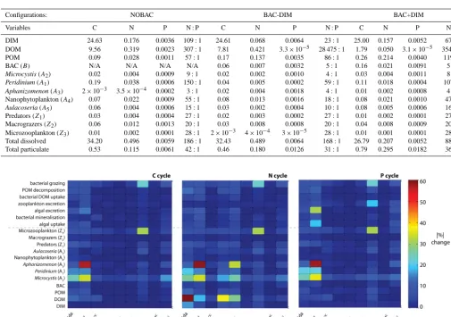
Several phytoplankton state variables, microzooplankton, and the various process pathways that connected them, were particularly sensitive to a number of key microbial loop pa-rameters (above the 20 % sensitivity level) (Fig. 3). In par-ticular, Peridinium and Microcystis were sensitive to the di-ameter of POM particles (dPOM) and the bacterial optimum
temperature (TOPTB). In addition todPOM and TOPTB, Mi-crocystis was sensitive to the zooplankton internal N : C
ra-tio (kZIN), and Aphanizomenon was also highly sensitive to
TOPTB(>50 %). Microzooplankton biomass, bacterial
graz-ing rates and zooplankton excretion rates were strongly sen-sitive toKZe(>30 %), with mild sensitivity todPOM,TOPTB,
KZIN and the half-saturation constant for bacterial function
(KB). The DOM concentration was sensitive to dPOM,
par-ticularly for N (> 50 %), and the maximum bacterial DOC uptake rate (µDECDOC), andKBandkZIN(>30 %). Looking
specifically at the process pathways, rates of algal excretion and algal uptake were sensitive toTOPTB, particularly in the
P cycle (>30 %). To summarise, the model output was most
sensitive to changes in the microbial loop parametersdPOM,
TOPTBandKZe, which had a significant effect on DOM, the
biomass of Peridinium, cyanobacteria, heterotrophic bacteria and microzooplankton.
3.3 Nutrient pools
The multi-annual and lake-wide nutrient pools were com-pared between the three microbial loop configurations to un-derstand how the microbial loop shifts the partitioning of nu-trients between different ecosystem compartments (Table 6). In each configuration, the stoichiometry of the POM, DOM and DIM pools was free to change, whereas the stoichiom-etry of zooplankton and bacteria were fixed, and the stoi-chiometry of phytoplankton was allowed to vary only within the range prescribed by the minimum and maximum param-eters of internal nutrient ratios. In each configuration, the DIC pools were similar, but the DOC pool in BAC + DIM was significantly lower (1.79 mg C L−1) than in NOBAC (9.56 mg C L−1) and BAC−DIM (7.81 mg C L−1). Simi-larly the DON and DOP pools in BAC + DIM were also lower than the corresponding pools in NOBAC and BAC−DIM, even though bacteria were able to take up DIN and DIP to meet their nutrient needs in this configuration. The N:P ra-tio of DOM in NOBAC was 307 : 1, and with bacteria in-cluded (both BAC−DIM and BAC + DIM), the N : P ra-tios increased significantly to 28 475 : 1 and 3543 : 1 respec-tively. For configurations with dynamically simulated bac-teria, the DIP pools in BAC−DIM (6.4×10⁻³mg P L−1) and BAC + DIM (5.2×10⁻³mg P L−1) were higher than that in NOBAC (3.6×10⁻³mg P L−1), suggesting enhanced P
availability for phytoplankton uptake when bacteria were present. The POM pools in BAC−DIM and BAC + DIM were also higher than those in NOBAC.
The biomass of bacteria and zooplankton varied in the dif-ferent microbial loop configurations, although the N : P sto-ichiometry of zooplankton and bacteria were fixed at 5 : 1 (bacteria), 27 : 1 (Z1, predatory zooplankton), 20 : 1 (Z2,
macrograzers), and 28 : 1 (Z3, microzooplankton). When
bacteria were able to uptake dissolved inorganic nutrients in BAC + DIM, the total bacterial biomass was 2.7 times larger than for BAC−DIM. For zooplankton, biomass of micro-zooplankton (Z3) was similar in NOBAC and BAC + DIM
and significantly lower in BAC−DIM. For predatory zoo-plankton (Z1) simulated biomass was greatest in NOBAC
and lowest in BAC + DIM and for macrograzers (Z2) it was
greatest in NOBAC and lowest in BAC−DIM.
The biomass and N : P stoichiometry of the five simulated phytoplankton groups each varied in response to the presence of bacteria in BAC−DIM and then with the addition of bac-terial uptake of inorganic nutrients in BAC + DIM. For
Mi-crocystis, Peridinium, nanophytoplankton and Aulacoseira,
Table 5. Statistical analysis of water quality variables in the three microbial loop configurations by ANOVA and Multiple Comparisons.
Dependent variable (I) Group (J) Group Mean Std. P value P value
difference error (pairwise) (between
(I – J) groups)
T NOBAC BAC−DIM −0.135 1.051 0.898 0.989
NOBAC BAC + DIM −0.140 1.051 0.894
BAC−DIM BAC + DIM −0.005 1.051 0.996
DO NOBAC BAC−DIM 0.052 0.236 0.826 0.237
NOBAC BAC + DIM 0.372 0.236 0.117
BAC−DIM BAC + DIM 0.320 0.236 0.178
NH4 NOBAC BAC−DIM 0.048∗ 0.006 0.000 0.000
NOBAC BAC + DIM 0.023∗ 0.006 0.000
BAC−DIM BAC + DIM −0.025∗ 0.006 0.000
NO3 NOBAC BAC−DIM 0.015∗ 0.005 0.002 0.003
NOBAC BAC + DIM 0.001 0.005 0.794
BAC−DIM BAC + DIM −0.014∗ 0.005 0.005
PO4 NOBAC BAC−DIM −0.000∗ 0.000 0.000 0.000
NOBAC BAC + DIM 0.000 0.000 0.958
BAC−DIM BAC + DIM 0.000∗ 0.000 0.000
TN NOBAC BAC−DIM −0.072∗ 0.015 0.000 0.000
NOBAC BAC + DIM 0.141∗ 0.015 0.000
BAC−DIM BAC + DIM 0.213∗ 0.015 0.000
TP NOBAC BAC−DIM −0.006∗ 0.001 0.000 0.000
NOBAC BAC + DIM −0.008∗ 0.001 0.000
BAC−DIM BAC + DIM −0.003∗ 0.001 0.005
Nanophytoplankton (A4) NOBAC BAC−DIM −0.004 0.007 0.555 0.126
NOBAC BAC + DIM −0.013∗ 0.007 0.048
BAC−DIM BAC + DIM −0.009 0.007 0.163
Microcystis (A2) NOBAC BAC−DIM 0.004 0.009 0.669 0.100
NOBAC BAC + DIM −0.014 0.009 0.107
BAC−DIM BAC + DIM −0.018∗ 0.009 0.042
Peridinium (A1) NOBAC BAC−DIM 0.321∗ 0.057 0.000 0.000
NOBAC BAC + DIM 0.161∗ 0.057 0.005
BAC−DIM BAC + DIM −0.161∗ 0.057 0.005
Aulacoseria (A5) NOBAC BAC−DIM 0.033 0.020 0.105 0.125
NOBAC BAC + DIM −0.005 0.020 0.795
BAC−DIM BAC + DIM −0.0385 0.020 0.060
Aphanizomenon (A3) NOBAC BAC−DIM −0.028∗ 0.005 0.000 0.000
NOBAC BAC + DIM −0.012∗ 0.005 0.009
BAC−DIM BAC + DIM 0.0156∗ 0.005 0.001
Predators (Z1) NOBAC BAC−DIM 0.345∗ 0.168 0.041 0.001
NOBAC BAC + DIM 0.617∗ 0.168 0.000
BAC−DIM BAC + DIM 0.272 0.168 0.107
Macrograzers (Z2) NOBAC BAC−DIM 0.585∗ 0.171 0.001 0.001
NOBAC BAC + DIM 0.552∗ 0.171 0.001
BAC−DIM BAC + DIM −0.033 0.171 0.848
Microzooplankton (Z3) NOBAC BAC−DIM 0.241∗ 0.068 0.000 0.001
NOBAC BAC + DIM 0.027 0.068 0.691
BAC−DIM BAC + DIM −0.214∗ 0.068 0.002
Table 6. Summary of average values (1997–2001) for C, N and P contents (mg L−1) and N : P molar ratios of the various food web compo-nents in different microbial loop configurations.
Configurations: NOBAC BAC-DIM BAC+DIM
Variables C N P N : P C N P N : P C N P N : P
DIM 24.63 0.176 0.0036 109:1 24.61 0.068 0.0064 23:1 25.00 0.157 0.0052 67:1
DOM 9.56 0.319 0.0023 307:1 7.81 0.421 3.3×10⁻⁵ 28 475:1 1.79 0.050 3.1×10⁻⁵ 3543:1
POM 0.09 0.028 0.0011 57:1 0.17 0.137 0.0035 86:1 0.26 0.214 0.0040 119:1
BAC (B) N/A N/A N/A N/A 0.06 0.007 0.0032 5:1 0.16 0.021 0.0091 5:1
Microcystis (A2) 0.02 0.004 0.0009 9:1 0.02 0.002 0.0010 4:1 0.03 0.004 0.0011 8:1
Peridinium (A1) 0.19 0.038 0.0006 150:1 0.04 0.005 0.0002 59:1 0.11 0.018 0.0004 107:1
Aphanizomenon (A3) 2×10⁻³ 3.5×10⁻⁴ 0.0002 3:1 0.02 0.004 0.0018 4:1 0.01 0.002 0.0008 4:1
Nanophytoplankton (A4) 0.07 0.022 0.0009 55:1 0.08 0.013 0.0016 18:1 0.08 0.021 0.0010 47:1
Aulacoseria (A5) 0.06 0.004 0.0006 15:1 0.03 0.002 0.0004 10:1 0.08 0.005 0.0006 16:1
Predators (Z1) 0.03 0.004 0.0004 27:1 0.02 0.003 0.0002 27:1 0.01 0.002 0.0001 27:1
Macrograzers (Z2) 0.06 0.012 0.0013 20:1 0.03 0.008 0.0008 20:1 0.04 0.008 0.0009 20:1
Microzooplankton (Z3) 0.01 0.002 0.0001 28:1 2×10⁻³ 4×10⁻⁴ 3×10⁻⁵ 28:1 0.01 0.001 0.0001 28:1
Total dissolved 34.20 0.496 0.0059 186:1 32.43 0.489 0.0064 168:1 26.79 0.207 0.0052 88:1
[image:13.612.51.560.96.439.2]Total particulate 0.53 0.115 0.0061 42:1 0.46 0.180 0.0126 31:1 0.79 0.295 0.0182 36:1
Figure 3. Local sensitivity analysis of simulated state variables and process rates for the C, N and P cycles presented as the lake average
absolute change after a±20 % parameter shift.
8 : 1; nanophytoplankton 47 : 1; Aulacoseira 16 : 1) were also higher than their N : P ratios in BAC−DIM (Peridinium 59 : 1; Microcystis 4 : 1; nanophytoplankton 18 : 1;
Aula-coseira 10 : 1). Conversely, for Aphanizomenon, simulated
biomass in BAC−DIM was higher than in BAC + DIM, but no change was observed in their molar N : P ratios (4 : 1). Overall, the total phytoplankton biomass in BAC + DIM was higher than that in BAC−DIM despite this simulation, in-cluding competition for inorganic nutrients by bacteria.
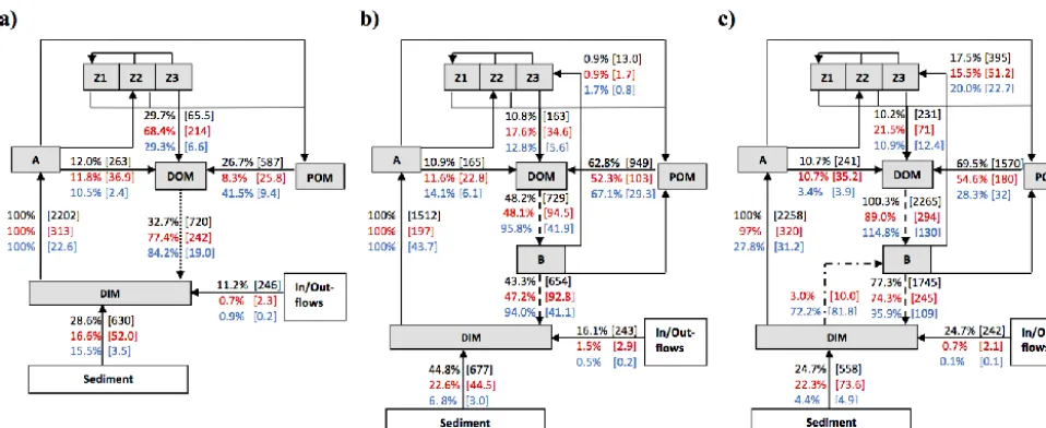
3.4 Nutrient fluxes
Simulated fluxes of C, N and P from the three microbial loop configurations representing the dominant C, N and P recy-cling pathways demonstrate significant differences in the rel-ative magnitude of bacterial mineralisation, zooplankton ex-cretion, zooplankton grazing, and bacterial competition with phytoplankton for inorganic nutrients (Fig. 4). The
simu-lated rate of algal primary productivity in the BAC + DIM and NOBAC configurations was higher than that simulated in BAC−DIM. Relative to the algal CO2fixation rate (defined
as 100 % for each simulation), in NOBAC, bacterial respira-tion returned 32.7 % of the total DIC assimilated by phyto-plankton, which was fuelled by DOC from microzooplankton excretion (29.7 %), hydrolysis of particulate detritus (26.7 %) and algal exudation (12.0 %); in BAC−DIM, bacterial res-piration returned 43.3 %, fuelled less by DOC from micro-zooplankton excretion (10.8 %), and more from hydrolysis of particulate detritus (62.8 %) and a similar amount from algal exudation (10.9 %); in BAC + DIM, the magnitude of bacterial respiration was 77.3 % of the total algal fixed car-bon, with similar proportions as in BAC−DIM; DOC from microzooplankton excretion (10.2 %), hydrolysis of particu-late detritus (69.5 %) and algal exudation (10.7 %).
Figure 4. Summary of simulated annual C (black), N (red) and P (blue) pathways for the three configurations: (a) NOBAC, (b) BAC−DIM, and (c) BAC + DIM. Note the dotted, dashed, and dash-dot lines emphasise configuration specific pathways. Selected fluxes relevant to the analysis are displayed as the lake-wide average % relative to the total DIM taken up by phytoplankton and bacteria (where relevant), with
the flux rate in brackets (×10−5mg L−1d−1).
in BAC−DIM. The algal DIN uptake percentage in BAC + DIM was 97.0 % relative to the 3.0 % uptake by bac-teria (i.e. rates are normalised by the total inorganic N uptake rate). In NOBAC, static mineralisation recycled 77.4 % of the total DIN taken up by phytoplankton, with microzooplankton excretion being the primary source of organic N with a sim-ilar relative magnitude (68.4 %). In BAC−DIM, bacterial mineralisation recycled 47.2 % of N, however only 17.6 % was supplied through microzooplankton excretion due to the lowerZ3biomass overall. In BAC + DIM, the bacterial
min-eralisation returned 74.3 %, with microzooplankton excre-tion supplying 21.5 %. As for carbon, in this simulaexcre-tion hy-drolysis of particulate detritus was the major source of labile organic nitrogen (>50 %) relative to that from zooplankton and phytoplankton excretion.
For phosphorus, the algal DIP uptake rate in BAC−DIM was higher than in BAC + DIM and NOBAC. In NOBAC, bacterial mineralisation replaced 84.2 % of total DIP assimi-lated by phytoplankton, and zooplankton excretion provided 29.3 % of this P to bacteria, with 41.5 % coming from POM hydrolysis and 10.5 % from algal exudation. In BAC−DIM, however, bacterial mineralisation recycled 94.0 %, with zoo-plankton excretion contributing just 12.8 % and the remain-der coming from POM hydrolysis (67.1 %) and algal ex-udation (14.1 %). When uptake of DIM by bacteria was simulated (BAC + DIM), DIP uptake shifted significantly to 27.8 % by algae and 72.2 % by bacteria, when normalised relative to the total PO4uptake rate. Of this total consumed
PO4, bacterial mineralisation was responsible for replacing
95.9 %, and DOM supplied by zooplankton excretion con-tributed 10.9 %, algal exudation concon-tributed 3.4 % and POM
hydrolysis 28.3 %. These fractions were less than that for C and N due to the large rate of supplementation of PO4.
Note that in all cases the amount of dissolved inorganic N and P that came from recycling compared to the inflows and sediment fluxes was very high. For example, the BAC + DIM model predicted that 95.9 % of dissolved inorganic P was sourced from recycling within the water column, only 4.4 % from the sediments, and less from the inflows. For N, the model predicted a reduced dependence on recycling (approx-imately 67 %), higher sediment flux (22.3 %) and a similar low contribution (0.7 %) from the inflows.
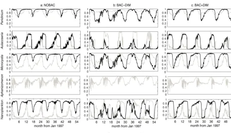
3.5 Patterns of phytoplankton biomass
In conjunction with variability in temperature, light and ver-tical mixing, changes in nutrient availability resulting from the dynamic nutrient recycling processes led to variation in phytoplankton nutrient uptake and their nutrient limitation functions, fa(N) and fa(P). The different patterns of sea-sonal variation in the nutrient limitation of the five simulated phytoplankton groups within the three model configurations highlight the potential for microbial loop sub-model struc-tures to influence phytoplankton growth response (Fig. 5). For example, Peridinium in NOBAC and BAC + DIM was predicted to have periodic N and P co-limitation, however, in BAC−DIM, N limitation was predicted to dominate most of the year. For Aulacoseira, in BAC−DIM, N and P co-limitation was experienced most of year, but in NOBAC and BAC + DIM, it displayed more P limitation. For
Microcys-tis, in NOBAC, P was the limiting factor for algal growth,
Figure 5. Comparison of nutrient limitation functions fa(N) and fa(P) respectively for the five simulated phytoplankton groups in a)
NOBAC, b) BAC−DIM and c) BAC + DIM.
experienced significant P limitation with an annual occur-rence of N and P co-limitation in spring. For the nanophyto-plankton, in NOBAC and BAC + DIM, its growth was P lim-ited with annual N and P co-limitation, but in BAC−DIM the growth switched between N limitation and P limitation annually. For Aphanizomenon, in all three configurations, P limitation dominated growth, since it is a N2-fixing species.
4 Discussion
4.1 Model performance and suitability
Given the complexity of interactions affecting phytoplankton succession and bloom dynamics, our ability to predict com-plex microbial food webs accurately remains a challenge. To date, there are limited modelling examples for a complete lake ecosystem that confidently simulate the successional dy-namics of phytoplankton and zooplankton at the level of mul-tiple trophic complexity as described here. This is due to the nonlinearity of these complex models and a large number of uncertain processes and parameters with limited validation data (Arhonditsis and Brett, 2004; Rigosi et al., 2010; Mooij et al., 2010). Nonetheless, the simulations were successful in capturing the seasonal dynamics and some of the interannual variation of the key plankton functional groups in Lake Kin-neret, though their absolute concentrations tended to be un-derpredicted. This is not unexpected given we have adopted a laterally averaged one-dimensional approach which is being
compared to inherently patchy field data, known to be partic-ularly relevant during Peridinium blooms (e.g. see Hillmer et al., 2008; Ng et al., 2011). However, the models were able to match the annual sequence and timing of the predicted peaks of these blooms, particularly the BAC + DIM configuration, which we consider to have the most biologically meaning-ful configuration. Within this simulation, the timescales of growth or decay of the biomass of biological variables gen-erally matched the observed data, and seasonal trends were accurately captured for physical and chemical variables since the model responds significantly to the strong seasonal forc-ing of the lake (Makler-Pick et al., 2011a). While we ac-knowledge further improvements could be made, the focus of our study was not specifically to find the model with the best fit to the data but to use the dynamic model to help us gain insights into the significance of microbial loop processes on phytoplankton growth in accordance with the approach suggested by van Nes and Scheffer (2005) for application of ecological models to explore theory. For this purpose, the model captures the variability of key physical, chemical and biological processes to a suitable level to allow us to inves-tigate the mechanisms governing the microbial interactions between the configurations.
configuration, with particular sensitivity noted in the con-centrations of inorganic nutrients available for phytoplank-ton growth. Generally, it was noted that in BAC−DIM in-organic nutrients were lower on average even though the to-tal nutrients were higher, due to a larger accumulation of or-ganic matter over time, indicating stoichiometric constraints reduce the efficiency of mineralisation (discussed below).
The differences in predicted surface nutrient concentra-tions between the simulaconcentra-tions led to the differences in pre-dicted plankton biomass and growth rates. The structure of the microbial loop model had a significant impact on the to-tal phytoplankton biomass, similar to the results of Faure et al. (2010) who explored the effect of microbial loop on DIN and phytoplankton for a coastal ecosystem. In this study, the analysis also includes phosphorus and several different functional groups of phytoplankton and zooplankton, and it was found that nutrients, Peridinium, Aphanizomenon and zooplankton were the main variables that showed sensitiv-ity to assumptions related to microbial loop configuration. Indeed, the evolution of the three model structures reported here was the product of adding process complexity based on perceived deficiencies in the calibration and this is reflected with BAC + DIM having the closest representation to the real lake ecosystem (see Appendix A).
We note numerous recent developments related to mod-elling the impact of food quality on grazing rates, related to both prey stoichiometry (Mitra et al., 2007) and prey fatty acid (HUFA) content (Perhar et al., 2013). Given the spe-cific focus of this study, our investigation has centred around the grazing rate of micrograzers who have grazed exclusively upon bacteria and have relatively stable biochemical compo-sition compared to phytoplankton (Sterner and Elser, 2002). Our grazing rates also become limited as zooplankton be-come unable to meet their stoichiometric requirements from prey, however, we acknowledge incorporating food quality dynamics in the general grazing formulation of the zooplank-ton as an important area of further model development. 4.2 Role of the microbial loop in regulating nutrient
flows
Specifically it was our aim to understand the mechanisms by which bacterial and microbial loop processes influence phy-toplankton via changes in carbon and nutrient cycles: (i) bac-terial mineralisation of organic nutrients, (ii) zooplankton ex-cretion of labile material, and (iii) bacterial competition with phytoplankton for inorganic nutrients when organic matter quality is poor (i.e. nutrient deplete). By comparing fluxes between pools of C, N and P we were able to gain insights into the role of the microbial loop in the recycling of nutri-ents.
Bacterial mineralisation had a strong regulatory effect on nutrient recycling, and the BAC + DIM model predicted that 70 % of N and around 95 % of P available for phytoplank-ton growth was from bacterial mineralisation of organic
mat-ter. These figures are based on a long-term simulation aver-age and relative contributions were found to vary seasonally in response to temperature and organic matter availability. However, in terms of carbon biomass, the bacterial popula-tion was found to be relatively stable. A key result emerging from the simulations is that the lowest concentration of DOC occurred in BAC + DIM, suggesting bacterial metabolism is enhanced when nutrient supplementation is accounted for. Although reports of bacterial growth being C limited have been made in many lakes (Coveney et al., 1992), bacteria in our simulations were mainly limited by P and also occasion-ally co-limited by N and P, as indicated by the relative use of inorganic nutrients. In the model, the DOM is assumed to be relatively labile, however, in reality different bioavailability of the various organic matter constituents may become lim-ited due to a lack of suitably bioavailable carbon. There is therefore scope for further extension of the model to under-stand how processes of mineralisation compare when multi-ple lability fractions of organic matter are considered.
It is well established that microzooplankton can transfer energy and nutrients via bacterial grazing to higher trophic levels due to their small size and high mass-specific graz-ing rates (Hart et al., 2000; Loladze et al., 2000), thereby playing an important role in carbon and nutrient recycling (Stone et al., 1993; Dolan, 1997; Hambright et al., 2007). In turn, larger zooplankton grazing on microzooplankton fur-ther provide organic matter for bacterial growth through ex-cretion of nutrient rich organic compounds (DOM) and fecal pellet production (POM) (Peduzzi and Herndl, 1992). From this point of view, the recycling of organic nutrients is fa-cilitated by bacterial consumers rather than bacteria them-selves, known as consumer-driven nutrient recycling (CNR) (Elser and Urabe, 1999). The model simulations presented in this study have allowed us to estimate the significance of this pathway and characterise the relative contributions of up-ward and downup-ward nutrient fluxes of these pathways. For example, in BAC + DIM, as a fraction of algal uptake, mi-crozooplankton excretion was predicted to account for 10 % of C, 22 % of N and 11 % of P returned for mineralisation, which was significantly larger than that supplied from algal excretion for N and P (but not for C), and therefore differ-ent from the relative proportions consumed through bacte-rial grazing (18 % for C, 15 % for N and 20 % for P). This highlights the dissimilarity and decoupling of the C, N and P cycles and the importance of nutrient adjustments that oc-cur during these microbial interactions, and is consistent with empirical work (Gaedke et al., 2002). The parameter sensi-tivity analysis indicated that both microzooplankton biomass and bacterial growth were particularly sensitive to the excre-tion fracexcre-tion of the ingested material (KZe) grazed by
mi-crozooplankton. Adjusting this excretion fraction parame-ter not only impacted their own biomass and grazing rates, but also impacted the biomass of other zooplankton groups and the phytoplankton community more broadly, including
zooplankton, any reduction in nutrient supply from micro-grazers leads to reduced P availability and ultimately reduced growth. These results reinforce that the interaction between phytoplankton and zooplankton is nonlinear and that there is both top-down (i.e. grazing-mediated) and bottom-up (i.e. microbial loop nutrient supply) processes shaping the phy-toplankton community. Interestingly, the smaller microzoo-plankton have a significant overall impact shaping the food web structure in the model simulations despite having the lowest biomass. These findings are in line with the empiri-cal studies of Hart et al. (2000) and Hambright et al. (2007), who highlighted the critical role of small micrograzers in the microbial loop processes. Since there exists a range of uncer-tainty surrounding the parameterisation of microzooplankton excretion, with large ranges being reported (Fasham et al., 1999; Faure et al., 2010), correct model parameterisation re-mains an important challenge for modellers.
In freshwater ecosystems, the concentration of DON can often be higher than that of DIN, and the DON pool plays an important role in providing N to both bacteria and algae (Berman, 1997, 2001; Berman and Bronk, 2003), though the latter is not considered in our model conceptualisation. In the present study, concentrations of DON were higher than those of DIN in NOBAC and BAC−DIM, which fits with observations by Berman and Bronk (2003). However, DON was lower than DIN in BAC + DIM where bacteria biomass and mineralisation rates were higher. As a result of increased DIN, DOP became the limiting factor when competition by bacteria for inorganic nutrients was included in the model configuration. Therefore, the variable stoichiometry of or-ganic matter, and different stoichiometric requirements of various process pathways, leads to a complex interplay be-tween the groups, and future studies should further consider the significance of organic matter stoichiometry, microzoo-plankton excretion rates and rates of nutrient immobilisation by bacteria when modelling planktonic food webs. We note the potential for N-fixation by heterotrophs, which is not con-sidered in our model, but expect the results would be rela-tively insensitive to this since bacteria are mostly P limited (refer to the high N:P ratios for DOM in Table 6).
4.3 Impact of the microbial loop on the phytoplankton community
Bacterial competition for inorganic nutrients has a two-fold effect on phytoplankton growth by limiting nutrient supply and regulating the N : P ratio of available nutrients. The time series of nutrient limitation functions for the five simulated phytoplankton groups for each of the three alternative mi-crobial loop configurations were used to decipher the effect of bacterial competition on phytoplankton growth. Whilst most freshwaters are considered to be P limited (Schindler et al., 2008), Elser et al. (2007) discusses that N and P co-limitation is commonly also prevalent. During the simulation period in this study, Lake Kinneret had an average TN : TP
ratio∼50 : 1, indicating strong P limitation as suggested by other authors. However, Gophen (2011) argues N limitation also occurs, potentially due to large fractions of unavail-able organic nitrogen distorting nutrient ratios (Ptanick et al., 2010). The model predictions of the five simulated phyto-plankton groups were predominantly P limited, with poten-tial for periodic N and P co-limitation depending on the mi-crobial loop configuration. When organic matter became P depleted, it could not support bacterial growth and therefore PO4supplementation of bacteria was evident in the increased
uptake rates (Fig. 4c). Bacteria generally have faster P up-take rates relative to phytoplankton (Berman, 1985), which in our model was captured by not limiting the rate of uptake of PO4by bacteria; as a result they were able to effectively
out-compete the phytoplankton. The model results indicate that this stoichiometric regulation of bacteria through DIM supplementation shifted patterns of phytoplankton nutrient limitation. Several phytoplankton groups experienced differ-ences in the degree of N and P limitation when bacteria were configured not to take up inorganic nutrients, as opposed to when bacteria were also consuming inorganic nutrients. The effect of competition on Peridinium manifested as N limita-tion when bacteria could not compete, but with competilimita-tion, periods of phosphorus limitation emerged following periods of accelerated growth. For Aulacoseira, the lack of bacterial competition for nutrients led to severe N limitation relative to predominant P limitation, coinciding with the period of the
Peridinium bloom. Similarly, for Microcystis and the mixed
nanophytoplankton community, stronger N limitation simu-lated in BAC−DIM switched to predominant P limitation in BAC + DIM.
It follows that bacteria-induced shifts in nutrient limitation can ultimately influence the overall biomass and composition of the phytoplankton community (Andersen et al., 2004). In-deed, here we noted relative differences in the simulated phy-toplankton biomass, and in particular, when competition with bacteria for inorganic nutrients was simulated, Peridinium dominated and Aulacoseira also occurred in significant num-bers. When this competition was not included, reduced
Peri-dinium and Aulacoseira biomass were evident, with a
corre-sponding significant increase in Aphanizomenon.
Microcys-tis were also slightly reduced and the nanophytoplankton
ap-peared to exhibit greater seasonality. Interestingly, focusing on the total phytoplankton biomass, the increased compe-tition for nutrients by bacteria somewhat paradoxically led to higher total phytoplankton biomass overall. Therefore the effect of the competition has a role in shaping the commu-nity structure and timing of blooms (see also Li et al., 2013), but overall the micrograzer driven recycling of N and P pos-itively promotes phytoplankton productivity.
Appendix A: Model validation and suitability assessment
[image:19.612.76.521.298.511.2]The performance of DYRESM-CAEDYM simulations has been reported in Gal et al. (2009) and Li et al. (2013) for the equivalent of our BAC + DIM simulation. The parameters for this simulation were derived from a manual calibration over the period 1997–1998, and error metrics were then compared over the full period 1997–2001. Parameter choice was based on a detailed synthesis of the large amount of laboratory and field process investigations conducted by the Kinneret Lim-nological Laboratory covering all aspects of model function (Table 2 in Gal et al., 2009). Fine-tuning of model param-eters was conducted within acceptable ranges for numerous parameters, however no formal calibration and error minimi-sation routine was used.
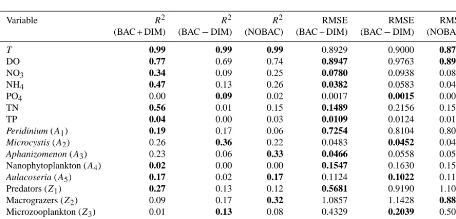
Table A1. Comparison ofR2and RMSE model validation metrics for the surface 10 m of Lake Kinneret for the main simulated variables. The best performing model configuration is highlighted bold.
Variable R2 R2 R2 RMSE RMSE RMSE
(BAC + DIM) (BAC−DIM) (NOBAC) (BAC + DIM) (BAC−DIM) (NOBAC)
T 0.99 0.99 0.99 0.8929 0.9000 0.8707
DO 0.77 0.69 0.74 0.8947 0.9763 0.8947
NO3 0.34 0.09 0.25 0.0780 0.0938 0.0815
NH4 0.47 0.13 0.26 0.0382 0.0583 0.0485
PO4 0.00 0.09 0.02 0.0017 0.0015 0.0017
TN 0.56 0.01 0.15 0.1489 0.2156 0.1548
TP 0.04 0.00 0.03 0.0109 0.0124 0.0159
Peridinium (A1) 0.19 0.17 0.06 0.7254 0.8104 0.8066
Microcystis (A2) 0.26 0.36 0.22 0.0483 0.0452 0.0472
Aphanizomenon (A3) 0.23 0.06 0.33 0.0466 0.0558 0.0542
Nanophytoplankton (A4) 0.02 0.00 0.00 0.1547 0.1630 0.1570
Aulacoseria (A5) 0.17 0.02 0.17 0.1124 0.1022 0.1114
Predators (Z1) 0.27 0.13 0.12 0.5681 0.9190 1.1029
Macrograzers (Z2) 0.09 0.17 0.32 1.0857 1.1428 0.8824
Microzooplankton (Z3) 0.01 0.13 0.08 0.4329 0.2039 0.5058
Bacteria (B) 0.02 0.01 N/A 0.0674 0.0643 N/A
The performance of BAC+DIM and the NOBAC and BAC−DIM simulations is summarised in Table A1 for 16 observed state variables. Data were available from weekly sampling at several locations and depths and used to gener-ate epilimnion and hypolimnion monthly averages. Note that only surface water data are compared here as no major dif-ferences were noted between the three simulations in the lake hypolimnion (except for NO3as seen in Fig. 2b).