The expected imprint of flux rope geometry on suprathermal electrons in magnetic clouds

Ann. Geophys., 27, 4057–4067, 2009 www.ann-geophys.net/27/4057/2009/

© Author(s) 2009. This work is distributed under the Creative Commons Attribution 3.0 License.

Annales

Geophysicae

The expected imprint of flux rope geometry on suprathermal

electrons in magnetic clouds

M. J. Owens1, N. U. Crooker2, and T. S. Horbury1

1_{Space and Atmospheric Physics, The Blackett Laboratory, Imperial College London, Prince Consort Road,} London SW7 2BW, UK

2_{Center for Space Physics, Boston University, Boston MA 02215, USA}

Received: 1 June 2009 – Revised: 20 August 2009 – Accepted: 14 October 2009 – Published: 26 October 2009

Abstract. Magnetic clouds are a subset of interplanetary coronal mass ejections characterized by a smooth rotation in the magnetic field direction, which is interpreted as a signa-ture of a magnetic flux rope. Suprathermal electron observa-tions indicate that one or both ends of a magnetic cloud typ-ically remain connected to the Sun as it moves out through the heliosphere. With distance from the axis of the flux rope, out toward its edge, the magnetic field winds more tightly about the axis and electrons must traverse longer magnetic field lines to reach the same heliocentric distance. This in-creased time of flight allows greater pitch-angle scattering to occur, meaning suprathermal electron pitch-angle distri-butions should be systematically broader at the edges of the flux rope than at the axis. We model this effect with an an-alytical magnetic flux rope model and a numerical scheme for suprathermal electron pitch-angle scattering and find that the signature of a magnetic flux rope should be observable with the typical pitch-angle resolution of suprathermal elec-tron data provided ACE’s SWEPAM instrument. Evidence of this signature in the observations, however, is weak, pos-sibly because reconnection of magnetic fields within the flux rope acts to intermix flux tubes.

Keywords. Interplanetary physics (Interplanetary magnetic fields; Energetic particles) – Solar physics, astrophysics, and astronomy (Flares and mass ejections)

1 Introduction

Coronal mass ejections (CMEs) are huge expulsions of solar plasma and magnetic field through the corona and out into the heliosphere, known to be the major cause of severe ge-omagnetic disturbances (e.g., Cane and Richardson, 2003).

Correspondence to: M. J. Owens ([email protected])

The interplanetary manifestations of CMEs (ICMEs) provide critical information about their magnetic configuration and orientation, which may prove key in constraining theories of CME initiation as well as aiding our understanding of the evolution of ejecta during their transit from the Sun to 1 AU. A variety of signatures are used to identify ICMEs from in situ data, including, but not limited to, low proton tem-peratures, counterstreaming suprathermal electrons, reduced magnetic field variance and enhanced ion charge states. See Wimmer-Schweingruber et al. (2006) for a more complete review. Magnetic clouds (MCs), a subset of ICMEs com-prising somewhere between a quarter to a third of all ejecta (e.g., Cane and Richardson, 2003), are further characterized by a smooth rotation in the magnetic field direction and an enhanced magnetic field magnitude (Burlaga et al., 1981). The field rotation has been attributed to a magnetic flux-rope (MFR, Lundquist, 1950) and commonly modeled as a constant-αforce-free MFR (Burlaga, 1988; Lepping et al., 1990), where currents are assumed to be field aligned andα

is the constant relating the current densityJ to the magnetic field vectorB. This enables single-point, in situ, time series to be interpreted in terms of the large-scale structure of the ejection.

The present study addresses the behavior of suprathermal electrons in magnetic clouds. In general, suprathermal elec-trons (i.e.,>70 eV) are of key interest to studies of the solar wind because the field-aligned “strahl” acts as an effective tracer of heliospheric magnetic field topology. A single strahl indicates open magnetic flux (Feldman et al., 1975; Rosen-bauer et al., 1977), while counterstreaming electrons (CSEs) often signal the presence of closed magnetic loops with both foot points rooted at the Sun (Gosling et al., 1987). A strong field-aligned strahl is expected and observed in the ambient solar wind near 1 AU, as even an initially isotropic distribu-tion near the Sun will undergo pitch-angle focusing due to conservation of magnetic moment in a decreasing magnetic field intensity. Strahl widths at 1 AU, however, are much

4058 M. J. Owens et al.: Suprathermal electron signatures of flux ropes broader than would be expected from focusing alone,

sug-gesting significant pitch-angle scattering must occur (e.g., Pilipp et al., 1987). Indeed, with increasing distance from the Sun, pitch-angle scattering becomes increasingly impor-tant because the rate of focusing decreases owing to the in-creasing angle between the spiraling magnetic field direction and intensity gradient (Owens et al., 2008). This results in the strahl width increasing with heliocentric distances (Ham-mond et al., 1996). For closed magnetic loops in an ICME, the antisunward motion of the loop apex will mean that in-transit scattering on the increasingly longer field-line will re-sult in eventual loss of the sunward beam and, hence, loss of the CSE signature, which has important implications for the interpretation of the solar cycle evolution of the heliospheric magnetic field (Owens and Crooker, 2006, 2007).

The flux rope structure of magnetic clouds means the field-line length is shortest at the axis of the MFR, increas-ing toward the edge as the field winds about the axis. In-direct evidence for the varying length of field lines in mag-netic clouds was found in the arrival-time dispersion of so-lar fso-lare electrons intermittently injected into the October 1995 magnetic cloud (Larson et al., 1997). (Chollet et al., 2007) recently used bursts within energetic particle disper-sions within an ICME to infer a jumbled mix of field-line lengths from∼1 to 3.5 AU. While energetic particle events can only be used to calculate field-line length in a very lim-ited number of ICMEs, field-line length should also have an effect on suprathermal electrons, which continually stream away from the Sun along field lines. Since the suprather-mal electron time of flight and, hence, pitch-angle scattering time, increases with field-line length, the strahl width should exhibit a characteristic signature as a flux rope convects past an observer at 1 AU.

To characterize the expected imprint of flux rope geome-try on suprathermal electron observations, we combine two forms of modeling. In Sect. 2, an analytical MFR model is used to calculate the length of magnetic field lines which connect an observer inside an MC to the Sun. In Sect. 3 a nu-merical model of suprathermal electron evolution is used to estimate the suprathermal electron strahl widths correspond-ing to the MFR magnetic field line lengths. Finally, in Sect. 5 we look for the predicted variation in strahl width in ACE ob-servations of magnetic clouds.

2 Magnetic flux rope model

The classic model for a magnetic cloud-associated flux rope, the constant-αforce-free flux rope (Burlaga, 1988; Lepping et al., 1990), assumes the magnetic cloud can locally be ap-proximated as a 2-dimensional cylindrical structure with a circular cross-section. The field is entirely axial at the center of the rope, becoming increasingly poloidal toward the outer edge. It is useful to define a parameterY, the ratio of the distance from the flux rope axis,r, to radius of the flux rope,

r0. The magnetic field of a force-free flux rope is then given by:

BAX(Y ) = B0J0(αY )

BPOL(Y )= ±B0J1(αY ) (1) whereBAXandBPOL are the magnetic field strengths along the axial and poloidal directions, respectively. The poloidal component takes positive or negative values depending on the sense of rotation of the magnetic field about the axis (i.e., the chirality of the flux rope). J0andJ1are zero and first order Bessel functions of the first kind, respectively. αis a constant which determines the outer edge of the flux rope. It is normally assumed to be 2.408, which effectively sets the outer edge of the flux rope at the point where the field first becomes entirely poloidal (Burlaga, 1988; Lepping et al., 1990).

The angle of the magnetic field to the axial direction,θ, is a function ofY:

tanθ= BAX

BPOL

= J0(αY )

J1(αY )

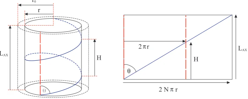
(2) We initially adopt this simple force-free geometry, later mod-ifying the model to incorporate effects which will substan-tially alter the estimate of field-line lengthLconnecting a 1-AU observer to the Sun. The left-hand panel of Fig. 1 defines the basic parameters: The rope is of radiusr0. At a distance rfrom the axis, the field takes the form of a helix about the axis, shown as the solid/dashed blue line, and makes an an-gleθ to the axis. The field makes one complete revolution about the axis in a height,H, along the axis. For an axis of lengthLAX, the field makesN revolutions (in the example shown,N∼1.8). The right-hand panel shows the curved face of the cylinder unrolled to form a flat plane. The relations betweenθ, H, LAX, N, r, r0and the length of the field line, L, are easier to visualize in this way. It can immediately be seen that the length of the field line is:

L=

q

L2_AX+(2N π r)2 ₍₃₎

and substitutingN H=LAXandH=2π r/tanθgives: L= LAX

cosθ (4)

Thus for a force-free flux rope, the length of the magnetic field line depends only onθ(which, in turn, is solely a func-tion ofY) and the length of the axial field line.Lis indepen-dent of the radius of the flux rope, as the number of revolu-tions per unit axial length is linearly related tor, the distance from the axis.

To estimate LAX, it is necessary to extend the 2-dimensional force-free model to a more global configuration. Assuming the flux rope plasma moves radially but the foot points of the flux rope remain connected to the Sun, as sug-gested by observations (Gosling et al., 1987), the axial field

M. J. Owens et al.: Suprathermal electron signatures of flux ropes 4059

Owens et al.: Suprathermal electron signatures of flux ropes 3

Fig. 1. The left-hand panel shows the cylindrical geometry implied by a force-free flux rope. The rope is of radiusr0. At a distancerfrom the axis, the field takes the form of a helix about the axis, shown as the solid/dashed blue line, and makes an angleθto the axis. The field makes one complete revolution about the axis in a height,H, along the axis. For an axis of lengthLAX, the field makesNrevolutions (in the case shownN ∼1.8). The right-hand panel shows the curved face of the cylinder unrolled to form a flat plane. The relations between

θ, H, LAX, N, r, r0and the length of the field line,Lare easier to visualize in this way.

where λ is the heliographic latitude, Ω = 2π/TSI D, and TSI Dis the sidereal rotation period of the Sun.LAXis there-fore given by:

LAX =

Z 1AU

0

dR

cosγ (6)

We now include the effect of expansion to allow for ax-ial curvature effects, and later in this Section, we incorporate a more realistic cross-sectional topology. Expansion is as-sumed to be self-similar about the axis, consistent with the linearly declining speed profiles observed within magnetic clouds (Owens et al., 2005). Thus while the axis of the flux rope moves antisunward at a cruise speedVC R, the edges of the flux rope move away from the axis at a speedVEX. The radius of the flux rope therefore varies with heliocentric dis-tance as:

r0 = VEXR

VC R

(7)

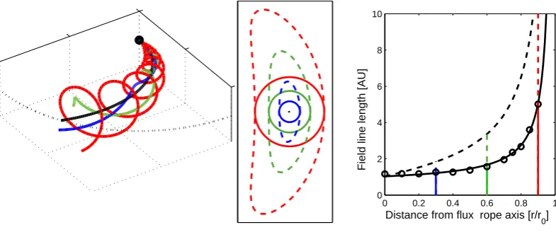
The left panel of Figure 2 shows a snapshot of the model flux rope using paramters VC R = 400km/s and VEX = 100km/s, typical magnetic cloud values (Owens et al., 2005). A heliocentric distance of 1 AU is shown as the black dotted curve, while the Sun is represented by a solid black circle. Only the half of the flux rope which provides the shortest magnetic connection between the Sun and 1 AU is shown. Field lines atY = 0, 0.3, 0.6 and 0.9 are shown by black, blue, green and red lines, respectively. Numerically inte-grating the distance along each helical path gives field-line lengths of 1.17, 1.23, 1.68 and 5.19 AU, respectively.

The open circles in the right panel of Figure 2 show the field-line length between 1 AU and the Sun as a function of

distance from the MFR axis. We find the following func-tional form, shown as the solid black line, adequately de-scribes the model points:

L[AU] = 0.631−_{0.1176 tan(}−_0.288Y −_{1.285) (8)}

Finally, we include the effect of MFR cross-sectional elon-gation in the non-radial direction. Magnetic clouds at 1 AU are known to be highly distorted from the circular cross-section assumed by the force-free approximation. Even if a flux rope has a circular cross-section near the Sun, it will become elongated in the non-radial direction by maintaining a constant angular width as it travels to 1 AU (e.g., Newkirk et al., 1981; McComas et al., 1988; Riley and Crooker, 2004; Owens, 2006). While it is difficult to analytically incorpo-rate this effect into the flux rope model presented here, the increase in field-line length can be approximated by consid-ering the increase in path length around the flux rope cross section. The solid lines in the middle panel of Figure 2 rep-resent model field non-elongated field lines forY =0.3, 0.6 and 0.9 for a force-free flux rope with its axis at 1 AU, which has traveled from the Sun atVC R= 400km/s and undergone expansion atVEX = 100km/s. Thus at 1 AU, the flux rope has a radial width of2VEXAU/VC R. The dashed lines rep-resent the equivalent cross-section for a flux rope with the same characteristic speeds and, hence, radial width at 1 AU as the force-free example but for a MFR which has under-gone the kinematic distortion expected from radial propaga-tion (Owens et al., 2006). The increase in field-line length per turn of the magnetic field about the axis is found to be ∼ _{1.7Y. This correction is applied to circular cross} sec-tion estimates of field line length to approximate the effect

Fig. 1. The left-hand panel shows the cylindrical geometry implied by a force-free flux rope. The rope is of radiusr0. At a distancerfrom

the axis, the field takes the form of a helix about the axis, shown as the solid/dashed blue line, and makes an angleθto the axis. The field makes one complete revolution about the axis in a height,H, along the axis. For an axis of lengthLAX, the field makesN revolutions (in

the case shownN∼1.8). The right-hand panel shows the curved face of the cylinder unrolled to form a flat plane. The relations between

θ, H, LAX, N, r, r0and the length of the field line,Lare easier to visualize in this way.

will lie predominantly along the Parker Spiral. Thus at a he-liocentric distanceR, the axis makes an angleγto the radial:

γ =arctan

R VCR

cosλ (5)

whereλis the heliographic latitude,=2π/TSID, andTSID is the sidereal rotation period of the Sun. LAX is therefore given by:

LAX=

Z 1 AU 0

dR

cosγ (6)

We now include the effect of expansion to allow for axial curvature effects, and later in this section, we incorporate a more realistic cross-sectional topology. Expansion is as-sumed to be self-similar about the axis, consistent with the linearly declining speed profiles observed within magnetic clouds (Owens et al., 2005). Thus while the axis of the flux rope moves antisunward at a cruise speedVCR, the edges of the flux rope move away from the axis at a speedVEX. The radius of the flux rope therefore varies with heliocentric dis-tance as:

r0= VEXR

VCR

(7) The left panel of Fig. 2 shows a snapshot of the model flux rope using paramters VCR=400 km/s and VEX=100 km/s, typical magnetic cloud values (Owens et al., 2005). A helio-centric distance of 1 AU is shown as the black dotted curve, while the Sun is represented by a solid black circle. Only the half of the flux rope which provides the shortest magnetic connection between the Sun and 1 AU is shown. Field lines atY=0, 0.3, 0.6 and 0.9 are shown by black, blue, green and red lines, respectively. Numerically integrating the distance

along each helical path gives field-line lengths of 1.17, 1.23, 1.68 and 5.19 AU, respectively.

The open circles in the right panel of Fig. 2 show the field-line length between 1 AU and the Sun as a function of dis-tance from the MFR axis. We find the following functional form, shown as the solid black line, adequately describes the model points:

L[AU] =0.631−0.1176 tan(−0.288Y −1.285) (8) Finally, we include the effect of MFR cross-sectional elon-gation in the non-radial direction. Magnetic clouds at 1 AU are known to be highly distorted from the circular cross-section assumed by the force-free approximation. Even if a flux rope has a circular cross-section near the Sun, it will become elongated in the non-radial direction by maintaining a constant angular width as it travels to 1 AU (e.g., Newkirk et al., 1981; McComas et al., 1988; Riley and Crooker, 2004; Owens, 2006). While it is difficult to analytically incorpo-rate this effect into the flux rope model presented here, the increase in field-line length can be approximated by consid-ering the increase in path length around the flux rope cross section. The solid lines in the middle panel of Fig. 2 rep-resent model field non-elongated field lines forY=0.3, 0.6 and 0.9 for a force-free flux rope with its axis at 1 AU, which has traveled from the Sun atVCR=400 km/s and undergone expansion atVEX=100 km/s. Thus at 1 AU, the flux rope has a radial width of 2VEXAU/VCR. The dashed lines rep-resent the equivalent cross-section for a flux rope with the same characteristic speeds and, hence, radial width at 1 AU as the force-free example but for a MFR which has under-gone the kinematic distortion expected from radial propaga-tion (Owens et al., 2006). The increase in field-line length per turn of the magnetic field about the axis is found to be

4060 M. J. Owens et al.: Suprathermal electron signatures of flux ropes

4

Owens et al.: Suprathermal electron signatures of flux ropes

0 0.2 0.4 0.6 0.8 1 0

2 4 6 8 10

Distance from flux rope axis [r/r 0]

Field line length [AU]

Fig. 2. The left panel shows a snapshot of the model magnetic flux rope. A heliocentric distance of 1 AU is shown as the black dotted curve, while the Sun is represented by a solid black circle. Only the half of the flux rope which provides the shortest magnetic connection between the Sun and 1 AU is shown. Field lines atY =0, 0.3, 0.6 and 0.9 are shown by black, blue, green and red lines, respectively. Solid lines in the center panel show a cross-section of the flux rope at 1 AU, while the dashed lines show how the cross-section is modified by kinematic distortion. The right panel shows the length of the field lines connecting 1-AU to the Sun as a function of distance from the flux rope axis, with solid (dashed) lines indicating a flux rope with a circular (kinematically-distorted) cross section.

of cross-sectional elongation, shown as the dashed line in the

right-hand panel of Figure 2. The best fit is given by:

L

[

AU

] = 1

.

07

−

₀

_.

_{20 tan(}

−

₀

_.

₂₈₈

_Y

−

₁

_.

₂₈₅₎

₍₉₎

3

Suprathermal electron evolution

The model of Owens et al. (2008) is used to determine the

ex-pected strahl width for a given pitch-angle scattering rate and

field-line length. This numerical scheme iteratively solves

electron heliocentric distance and pitch-angle, allowing for

movement along the magnetic field direction and

convec-tion with the bulk solar wind moconvec-tion. Electrons undergo the

competing effects of adiabatic focusing from conservation

of magnetic moment and pitch-angle scattering toward an

isotropic distribution. The radial evolution of the

suprather-mal electron strahl width in the fast solar wind can be well

matched by this scheme (Owens et al., 2008).

In this study we use a grid of 500 cells in electron

pitch-angle (

P A

) space, equally spaced in

cos

P A

. Grid cells are

spaced by 0.01 AU in heliocentric distance. Although we are

interested in strahl widths at 1 AU, the simulation domain

extends out to 2 AU to capture the contribution of electrons

which are scattered to pitch angles greater than 90

and thus

propagate sunward. A time step of 100 seconds and a

so-lar wind speed (

V

) of 400 km/s are used. Electron

en-ergy is set at 272eV, as this is the center value of the most

commonly-used suprathermal electron energy band for

char-acterizing the strahl (e.g., Anderson et al., 2008).

The model field-line length is adjusted by over- or

under-winding a Parker Spiral magnetic field (though the bulk solar

wind speed experienced by electrons is held constant at 400

km/s). We choose not to use the exact MFR field

geome-try outlined in the previous Section, as it would require

ex-tremely high spatial and temporal resolution due to the large

gradients in the magnetic field direction, making it

compu-tationally prohibitive. Note that the electron model used in

this study only accounts for the two major effects:

Chang-ing magnetic field strength, which adiabatically focuses

elec-trons, and time of flight, which allows greater pitch-angle

scattering to occur. The orientation of the field does not have

a direct effect, other than directing electrons into regions of

different field strength. Thus while the over/under-wound

Parker spiral field will not capture the repeated adiabatic

focusing and defocusing of electrons traversing the helical

magnetic field of a flux rope, it will capture the net

pitch-angle focusing and the net amount of scattering experienced

by the electrons.

Pitch-angle scattering is performed in an ad-hoc manner,

by Gaussian broadening the PA distribution at each time step,

pushing the distribution toward isotropy. A broadening

fac-tor of

σ

= 0

.

0014

applied each second was found to best

match the observed strahl width in the fast solar wind

(Ham-Fig. 2. The left panel shows a snapshot of the model magnetic flux rope. A heliocentric distance of 1 AU is shown as the black dotted curve,

while the Sun is represented by a solid black circle. Only the half of the flux rope which provides the shortest magnetic connection between the Sun and 1 AU is shown. Field lines atY=0, 0.3, 0.6 and 0.9 are shown by black, blue, green and red lines, respectively. Solid lines in the center panel show a cross-section of the flux rope at 1 AU, while the dashed lines show how the cross-section is modified by kinematic distortion. The right panel shows the length of the field lines connecting 1-AU to the Sun as a function of distance from the flux rope axis, with solid (dashed) lines indicating a flux rope with a circular (kinematically-distorted) cross section.

∼1.7Y. This correction is applied to circular cross section estimates of field line length to approximate the effect of cross-sectional elongation, shown as the dashed line in the right-hand panel of Fig. 2. The best fit is given by:

L[AU] =1.07−0.20 tan(−0.288Y −1.285) (9)

3 Suprathermal electron evolution

The model of Owens et al. (2008) is used to determine the ex-pected strahl width for a given pitch-angle scattering rate and field-line length. This numerical scheme iteratively solves electron heliocentric distance and pitch-angle, allowing for movement along the magnetic field direction and convec-tion with the bulk solar wind moconvec-tion. Electrons undergo the competing effects of adiabatic focusing from conservation of magnetic moment and pitch-angle scattering toward an isotropic distribution. The radial evolution of the suprather-mal electron strahl width in the fast solar wind can be well matched by this scheme (Owens et al., 2008).

In this study we use a grid of 500 cells in electron pitch-angle (P A) space, equally spaced in cosP A. Grid cells are spaced by 0.01 AU in heliocentric distance. Although we are interested in strahl widths at 1 AU, the simulation domain extends out to 2 AU to capture the contribution of electrons which are scattered to pitch angles greater than 90◦_{and thus} propagate sunward. A time step of 100 s and a solar wind speed (VSW) of 400 km/s are used. Electron energy is set at 272 eV, as this is the center value of the most commonly-used suprathermal electron energy band for characterizing the strahl (e.g., Anderson et al., 2008).

The model field-line length is adjusted by over- or under-winding a Parker Spiral magnetic field (though the bulk

so-lar wind speed experienced by electrons is held constant at 400 km/s). We choose not to use the exact MFR field geom-etry outlined in the previous section, as it would require ex-tremely high spatial and temporal resolution due to the large gradients in the magnetic field direction, making it compu-tationally prohibitive. Note that the electron model used in this study only accounts for the two major effects: Chang-ing magnetic field strength, which adiabatically focuses elec-trons, and time of flight, which allows greater pitch-angle scattering to occur. The orientation of the field does not have a direct effect, other than directing electrons into regions of different field strength. Thus while the over/under-wound Parker spiral field will not capture the repeated adiabatic focusing and defocusing of electrons traversing the helical magnetic field of a flux rope, it will capture the net pitch-angle focusing and the net amount of scattering experienced by the electrons.

Pitch-angle scattering is performed in an ad-hoc manner, by Gaussian broadening the PA distribution at each time step, pushing the distribution toward isotropy. A broaden-ing factor of σ=0.0014 applied each second was found to best match the observed strahl width in the fast solar wind (Hammond et al., 1996; Owens et al., 2008). In this study, three levels of scattering are used: The fast solar wind level, taken as “medium” scattering, and “low” and “high” levels of scattering at half and double this value, respectively. The model width at 1 AU is then computed from the model PA distribution using the same fitting procedure as Hammond et al. (1996) and Owens et al. (2008). Suprathermal electron pitch-angle distributions are fit with the following functional form:

M. J. Owens et al.: Suprathermal electron signatures of flux ropes 4061

6 Owens et al.: Suprathermal electron signatures of flux ropes

0 5 10 15

20 30 40 50 60 70 80 90 100 110

Field line length [AU]

Strahl width [degrees]

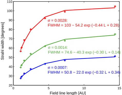
σ = 0.0028:

FWHM = 103 − 54.2 exp (−0.44 L + 0.28)

σ = 0.0007:

FWHM = 50.8 − 22.0 exp (−0.32 L + 0.34)

σ = 0.0014:

FWHM = 74.6 − 40.3 exp (−0.30 L + 0.14)

Fig. 3. The effect of varying scattering rate and field-line length on the strahl FWHM at 1 AU. As expected, the increased time of flight along longer field lines results in a broader strahl. AsL→ ∞, however, the strahl width asymptotes well before isotropy is achieved. This

is because the time of flight of the electrons, from the Sun to the observer, has a maximum value of1_AU/VSWdue to the convection of the magnetic field line with the bulk solar wind.

5 Observations

5.1 Case studies

In this Section we look for the expected suprathermal electron signature of a magnetic flux rope in the ACE SWEPAM (McComas et al., 1998) data. Three magnetic clouds, listed as A, B, and C in Table 1, have been selected from the Cane and Richardson (2003) ICME list (available at http://www.ssg.sr.unh.edu/mag/ace/ACElists/ICMEtable.html) for their classic form and range of strahl widths.

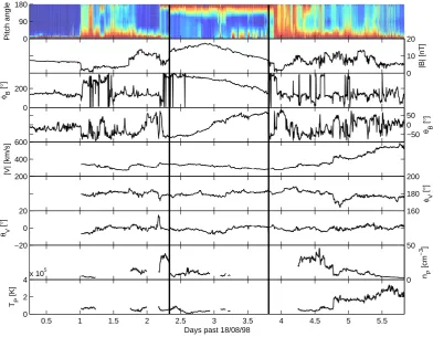
Figure 6 shows data from Event A. There is a clear ro-tation in the magnetic field direction, indicative of a mag-netic flux rope. This is reflected in the ratios of the eigen-vectors in the magnetic field variance directions listed in Ta-ble 1 (High ratios, typically>4, indicate strong flux rope signatures (e.g., Bothmer and Schwenn, 1998)). Fitting the Owens et al. (2006) magnetic cloud model to the observed time series suggests the spacecraft passed close to the axis (Y = 0.12). Despite the apparently near-perfect conditions, the expected signature of a dip in suprathermal electron strahl width is not present. This conclusion would not change if al-ternative cloud boundaries were chosen as the strahl observed immediately before and after the period of magnetic field ro-tation is narrower, not wider, than inside the event. Note, however, that in the ambient solar wind, the strahl width is generally broader than in the magnetic cloud. As the field-line length is expected to be shorter in the ambient solar wind than in the cloud, pitch-angle scattering must be greatly

sup-pressed in this magnetic cloud compared to ambient condi-tions. See, however, Event B.

The magnetic field data for Events B and C are not shown, but Table 1 lists the ratios of the eigenvalues in the variance directions to quantify the quality of the flux rope signature. Also listed are model values ofY, the closest approach of the spacecraft to the axis, which are both small.

The top panels of Figure 7 show the 272 eV suprather-mal electron pitch-angle distributions, norsuprather-malized at each time step, for the three magnetic cloud intervals. For each event, we compute the flux in the 0◦and 180◦strahls (i.e., K1 in Equation 10) throughout the magnetic cloud inter-val, and define the dominant strahl as that with the highest flux. For Event A the dominant strahl is at 180◦pitch an-gle, with an order of magnitude higher electron flux than any0◦ _{strahl. We note, however, that the dominant strahl}

is not always as easy to define, particularly in events with a strong counterstreaming signature. For event A, there is a clear broadening of the strahl near the center of the cloud and evidence of counterstreaming near the rear of the cloud. This intermingling of apparently open and closed fields is not uncommon within magnetic clouds (e.g., Crooker et al., 2008). The dominant strahl for Event B is at 0◦pitch an-gle. It is much broader than the strahl in Event A. Finally, Event C has a very narrow strahl at 180◦_{, close to, but}

above the pitch-angle resolution of the standard SWEPAM suprathermal electron data, with intermittent counterstream-ing throughout the cloud. These three events highlight the large event-to-event variability in the suprathermal electron

Fig. 3. The effect of varying scattering rate and field-line length on

the strahl FWHM at 1 AU. As expected, the increased time of flight along longer field lines results in a broader strahl. AsL→∞, how-ever, the strahl width asymptotes well before isotropy is achieved. This is because the time of flight of the electrons, from the Sun to the observer, has a maximum value of 1 AU/VSW due to the con-vection of the magnetic field line with the bulk solar wind.

j (P A)=K0+K1exp

"

−P A2 K3

#

(10)

wherej (P A)is the differential electron flux at pitch angle

P A,K0describes the electron density of the halo andK3 de-termines the width of the strahl (the full width at half maxi-mum is given by FWHM=2√(ln 2)K3).K1is the maximum electron density of the strahl aboveK0.

Figure 3 shows the effect of varying scattering rate and field-line length on the strahl width at 1 AU. As expected, the increased time of flight along longer field lines results in a broader strahl. The three levels of scattering are fit with an exponential function, to give the following relations:

σ =0.0007[s−1] : (11)

FWHM(◦)=51−_{22 exp [0}.34−0.32LAU]

σ =0.0014[s−1] :

FWHM(◦)=75−40 exp [0.14−0.30LAU]

σ =0.0028[s−1] :

FWHM(◦)=103−54 exp [0.28−0.44LAU] whereLAU is the field-line length in AU. AsL→∞, how-ever, the strahl width asymptotes well before isotropy is achieved. This is because the total radial velocity of an elec-tron is given by VSW+Vkcosγ, where Vk is the electron speed along the magnetic field direction andγ is the angle of the field to the radial direction. The first term represents the propagation of magnetic field lines out from the Sun at the bulk solar wind speed. Thus regardless of the field-line

length, the maximum time of flight of an anti-sunward prop-agating electron to a 1−AUobserver will be 1 AU/VSW.

4 Model time series

We now combine the MFR and electron scattering models to produce the expected suprathermal electron time series at 1 AU. The first step is to generate field-line lengths connect-ing an observer at 1 AU to the Sun as a magnetic cloud prop-agates out through the heliosphere. As the expansion speed of magnetic clouds is often a significant fraction of the cruise speed (Owens et al., 2005), we build up a true time series of the model parameters by time evolving past a fixed point at 1 AU rather than take a radial slice through a snapshot of the MFR model.

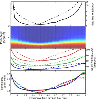
For this initial time series, the observer is assumed to pass directly through the axis of the flux rope (i.e., throughY=0), but this is later relaxed when comparing to observations. A cruise (expansion) speed of 400 (100) km/s is used. The top panel of Fig. 4 shows the resulting time series of the mag-netic field line length in the flux rope connecting the 1-AU observer to the Sun, with solid (dashed) lines representing a circular cross-section (kinematically distorted) flux rope. Note the logarithmic scale on the y-axis. The second panel shows the result of combining the field-line length with the scattering code to produce a time series of 272 eV electron pitch-angle density at 1 AU. This type of plot is commonly used to display suprathermal electron observations. It shows the electron flux at a given energy level, normalized to the maximum and minimum densities at each time step, as a function of pitch angle and time. The strahl width exhibits a clear broad-narrow-broad trend. The third panel shows the computed strahl widths for high (red), medium (green) and low (blue) levels of pitch-angle scattering, for circular cross-section (solid) and kinematically-distorted (dashed) flux rope models. The bottom panel shows the strahl width normalized to the mean strahl width in the event. This normalized width is independent of the scattering rate and only a function of field-line length.

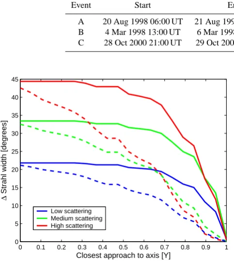
The maximum change in strahl width expected through a MFR,1FWHM, is a useful parameter for assessing whether or not the flux rope signature should be observable with a given instrument: If 1FWHM is below the pitch-angle resolution, the effect cannot be measured. Figure 5 shows

1FWHM as a function of the closest approach of the ob-server to the axis of a MFR (i.e., the minimum value ofY, often referred to as the “impact parameter”). The color code is the same as in Fig. 4. Very few magnetic clouds are actu-ally encountered “on axis”, and thus the minimum value ofY

sampled by the observer is normally>0. Although1FWHM drops with impact parameter, there is still significant varia-tion in the strahl width even when the observer passes far (e.g.,Y∼0.5) from the axis of the flux rope, particularly for higher scattering rates. For extreme glancing encounters of

4062 M. J. Owens et al.: Suprathermal electron signatures of flux ropes

Owens et al.: Suprathermal electron signatures of flux ropes

7

0.2 0.4 0.6 0.8 1

0 90 180

Pitch Angle [degrees]

0.1 0.2 0.3 0.4 0.5 0.6 0.7 0.8 0.9 1

40 60 80 100

Strahl width at 1 AU [degrees]

0 0.1 0.2 0.3 0.4 0.5 0.6 0.7 0.8 0.9 1

0.8 1 1.2 1.4

Fraction of time through flux rope

Normalised strahl width

1 2 3 5 10 15

Field line length [AU]

Fig. 4. The model flux rope field-line lengths and expected suprathermal electron signatures. Solid (dashed) lines represent a circular

cross-section (kinematically-distorted) flux rope. The top panel shows a time series of field line length connecting an observer to the Sun.

Note the logarithmic scale on the y-axis. The second panel shows the normalized 272eV electron pitch-angle density, which exhibits a clear

broad-narrow-broad trend through the flux rope. The third panel shows strahl FWHM for high (red), medium (green) and low (blue) levels

of pitch-angle scattering. The bottom panel shows the strahl width normalized to the mean width, in the same format.

Event

Start

End

λ

/λ

λ

/λ

Y

A

20/8/1998 0600 UT

21/8/1998 2000 UT

23.4

3.75

0.12

B

4/3/1998 1300 UT

6/3/1998 0900 UT

15.5

4.13

0.10

C

28/10/2000 2100 UT

29/10/2000 2200 UT

3.15

7.03

0.27

Table 1. Start and end times of three examples of classic magnetic clouds selected from the Cane and Richardson (2003) ICME list.

λ

/λ

and

λ

/λ

are the ratios of magnetic field variances in the variance directions.

Y

is the closest approach of the

observing spacecraft to the flux rope axis inferred from a flux rope model fit.

properties of magnetic clouds (see also Anderson et al.,

2008).

The black lines in the middle panels of Figure 7 show the

strahl width, computed from the observed pitch-angle

distri-butions using Equation 10. Solid (dashed) colored lines show

the model strahl widths for circular (kinematically-distorted)

cross-section flux ropes using the inferred values of

Y

listed

in Table 1. Low, medium and high levels of pitch-angle

scat-tering are shown by the blue, green and red lines,

respec-tively. The bottom panels show the normalized strahl widths

in the same format. In all three magnetic clouds, the expected

imprint of flux rope geometry on the suprathermal electrons

is absent.

5.2

Statistical survey

In this Section we statistically survey magnetic cloud

suprathermal electron profiles. All the events classified as

magnetic clouds in the Cane and Richardson (2003) ICME

list observed between 1998 and 2007 (74 events) are

cross-section (kinematically-distorted) flux rope. The top panel shows a time series of field line length connecting an observer to the Sun. Note the logarithmic scale on the y-axis. The second panel shows the normalized 272eV electron pitch-angle density, which exhibits a clear broad-narrow-broad trend through the flux rope. The third panel shows strahl FWHM for high (red), medium (green) and low (blue) levels of pitch-angle scattering. The bottom panel shows the strahl width normalized to the mean width, in the same format.

flux ropes, where the minimumYintersected by an observing spacecraft is>0.5, the field rotation signature will be signif-icantly weaker, and the event is unlikely to be classified as a magnetic cloud.

The SWEPAM instrument (McComas et al., 1998) on the ACE spacecraft collects electron data in approximately 6◦×20◦angular bins. For the standard SWEPAM suprather-mal electron data set, the data is then binned into 9◦ resolu-tion in pitch-angle space. Figure 5 shows that under most cir-cumstances the difference in strahl width across a flux rope should be more than twice this SWEPAM resolution angle and thus clearly observable.

5 Observations

5.1 Case studies

In this section we look for the expected suprathermal electron signature of a magnetic flux rope in the ACE SWEPAM (Mc-Comas et al., 1998) data. Three magnetic clouds, listed as A, B, and C in Table 1, have been selected from the Cane and Richardson (2003) ICME list (available at http://www.ssg.sr. unh.edu/mag/ace/ACElists/ICMEtable.html) for their classic form and range of strahl widths.

Figure 6 shows data from Event A. There is a clear rotation in the magnetic field direction, indicative of a magnetic flux rope. This is reflected in the ratios of the eigenvectors in the magnetic field variance directions listed in Table 1 (High ra-tios, typically>4, indicate strong flux rope signatures (e.g., Bothmer and Schwenn, 1998)). Fitting the Owens et al.

M. J. Owens et al.: Suprathermal electron signatures of flux ropes 4063

Table 1. Start and end times of three examples of classic magnetic clouds selected from the Cane and Richardson (2003) ICME list.

λINT/λMINandλMAX/λINTare the ratios of magnetic field variances in the variance directions.Yis the closest approach of the observing

spacecraft to the flux rope axis inferred from a flux rope model fit.

Event Start End λINT/λMIN λMAX/λINT Y

A 20 Aug 1998 06:00 UT 21 Aug 1998 20:00 UT 23.4 3.75 0.12

B 4 Mar 1998 13:00 UT 6 Mar 1998 09:00 UT 15.5 4.13 0.10

C 28 Oct 2000 21:00 UT 29 Oct 2000 22:00 UT 3.15 7.03 0.27

8 Owens et al.: Suprathermal electron signatures of flux ropes

0 0.1 0.2 0.3 0.4 0.5 0.6 0.7 0.8 0.9 1 0

5 10 15 20 25 30 35 40 45

∆

Strahl width [degrees]

Closest approach to axis [Y]

Low scattering Medium scattering High scattering

Fig. 5. The maximum expected change in strahl width, a measure of how readily the flux rope signature should be observable, as a function

of the closest approach of the observer to the axis of the event (i.e., the minimum value ofY, often referred to as the “impact parameter”). The color code is the same as Figure 4. Although∆FWHM drops off with impact parameter, there is significant variation in the strahl width even when the observer passes far (e.g.,Y ∼0.5) from the axis of the flux rope.

sidered. For each event, the dominant strahl is determined within the given magnetic cloud boundaries, and the strahl width is fit using Equation 10. The left-hand panel of Figure 8 shows a superposed epoch plot of the strahl width as a func-tion of time, expressed as a fracfunc-tion of the event’s durafunc-tion. The colored lines show the model predictions in the same format as Figure 4, assuming on-axis encounters of magnetic clouds. In this view, which covers a wide range of strahl widths to accommodate the full range of scattering constants, the superposed epoch plot shows little variation, and the pre-dicted flux rope signature does not appear to be present. In contrast, the right-hand panel shows the same strahl width data normalized to the mean strahl width within an event. In this format, there is some evidence of the predicted trend in the observations, with an asymmetric dip in strahl width to-ward the center of magnetic clouds. The trend, however, is much weaker than predicted by the models.

6 Conclusions

Inside a magnetic flux rope, the varying pitch of the helical field lines means that their lengths vary substantially between the Sun and an observer. This, in turn, affects the suprather-mal electron time of flight and, hence, the pitch-angle scat-tering time. The strahl width observed as a flux rope convects past a 1-AU observer is therefore expected to exhibit a char-acteristic variation from a broad strahl at the outer edge that

narrows toward the axis and then broadens again toward the opposite edge.

We have combined an analytical magnetic flux rope model with a numerical suprathermal electron scattering code to estimate this expected imprint of flux rope geometry on suprathermal electrons in magnetic clouds. The field-line length is found to increase by more than an order of mag-nitude from the axis to the edge of the flux rope. The as-sociated variation in strahl width at1AU, however, is not as extreme because convection of magnetic field lines with the ambient solar wind imposes a maximum electron time of flight of1AU/VSW, independent of field-line length.

The expected variation in strahl width is found to be de-pendent on the level of scattering in the sense that magnetic clouds with broader strahls throughout should exhibit a more pronounced flux rope imprint. If, however, the strahl width is normalised to the average strahl width observed in the event, the flux rope signature is independent of the scattering rate. For the flux rope signature to be observable, the maximum change in strahl width through a flux rope,∆F W HM, must be above the pitch-angle resolution of the instrument used to measure the suprathermal electron distribution. For the stan-dard ACE SWEPAM data set (McComas et al., 1998), this cut-off point is 9◦. Even for magnetic cloud encounters far from the axis of the flux rope, this signature should, in prin-ciple, be observable for a range of scattering rates.

Suprathermal electron observations for three classic exam-ples of magnetic clouds were examined. There was large

Fig. 5. The maximum expected change in strahl width, a measure of

how readily the flux rope signature should be observable, as a func-tion of the closest approach of the observer to the axis of the event (i.e., the minimum value ofY, often referred to as the “impact pa-rameter”). The color code is the same as Fig. 4. Although1FWHM drops off with impact parameter, there is significant variation in the strahl width even when the observer passes far (e.g.,Y∼0.5) from the axis of the flux rope.

(2006) magnetic cloud model to the observed time series suggests the spacecraft passed close to the axis (Y=0.12). Despite the apparently near-perfect conditions, the expected signature of a dip in suprathermal electron strahl width is not present. This conclusion would not change if alternative cloud boundaries were chosen as the strahl observed imme-diately before and after the period of magnetic field rotation is narrower, not wider, than inside the event. Note, however, that in the ambient solar wind, the strahl width is generally broader than in the magnetic cloud. As the field-line length is expected to be shorter in the ambient solar wind than in the cloud, pitch-angle scattering must be greatly suppressed in this magnetic cloud compared to ambient conditions. See, however, Event B.

The magnetic field data for Events B and C are not shown, but Table 1 lists the ratios of the eigenvalues in the variance directions to quantify the quality of the flux rope signature.

Also listed are model values ofY, the closest approach of the spacecraft to the axis, which are both small.

The top panels of Fig. 7 show the 272 eV suprathermal electron pitch-angle distributions, normalized at each time step, for the three magnetic cloud intervals. For each event, we compute the flux in the 0◦ and 180◦strahls (i.e.,K1 in Eq. 10) throughout the magnetic cloud interval, and define the dominant strahl as that with the highest flux. For Event A the dominant strahl is at 180◦pitch angle, with an order of magnitude higher electron flux than any 0◦strahl. We note, however, that the dominant strahl is not always as easy to define, particularly in events with a strong counterstreaming signature. For Event A, there is a clear broadening of the strahl near the center of the cloud and evidence of counter-streaming near the rear of the cloud. This intermingling of apparently open and closed fields is not uncommon within magnetic clouds (e.g., Crooker et al., 2008). The dominant strahl for Event B is at 0◦ pitch angle. It is much broader than the strahl in Event A. Finally, Event C has a very narrow strahl at 180◦, close to, but above the pitch-angle resolution of the standard SWEPAM suprathermal electron data, with intermittent counterstreaming throughout the cloud. These three events highlight the large event-to-event variability in the suprathermal electron properties of magnetic clouds (see also Anderson et al., 2008).

The black lines in the middle panels of Fig. 7 show the strahl width, computed from the observed pitch-angle distri-butions using Eq. (10). Solid (dashed) colored lines show the model strahl widths for circular (kinematically-distorted) cross-section flux ropes using the inferred values ofY listed in Table 1. Low, medium and high levels of pitch-angle scat-tering are shown by the blue, green and red lines, respec-tively. The bottom panels show the normalized strahl widths in the same format. In all three magnetic clouds, the expected imprint of flux rope geometry on the suprathermal electrons is absent.

5.2 Statistical survey

In this section we statistically survey magnetic cloud suprathermal electron profiles. All the events classified as magnetic clouds in the Cane and Richardson (2003) ICME list observed between 1998 and 2007 (74 events) are con-sidered. For each event, the dominant strahl is determined

4064 M. J. Owens et al.: Suprathermal electron signatures of flux ropes

Owens et al.: Suprathermal electron signatures of flux ropes 9

0 90 180

Pitch angle

0 10 20

|B| [nT]

0 200

φB

[

°

]

−50 0 50

θB

[

°

]

200 400 600

|V| [km/s]

160 180 200

φV

[

°

]

−20 0 20

θV

[

°

]

0 50

nP

[cm

−3

]

0.5 1 1.5 2 2.5 3 3.5 4 4.5 5 5.5

0 2 4x 10

5

TP

[K]

Days past 18/08/98

Fig. 6. Event A: A magnetic cloud observed in August 1998. The panels, from top to bottom are: The 272eV electron pitch-angle distribution,

the magnetic field magnitude, the in- and out-of-ecliptic magnetic field angles, the solar wind flow speed, the in- and out-of-ecliptic solar wind flow angles, the proton density and proton temperature. The boundaries of the magnetic cloud are shown by the solid vertical lines. A kinematically-distorted flux rope model fit to the observed magnetic field time series (not shown), suggests the axis of the flux rope passed withinr/r0= 0.12of ACE at the point of closest approach. The dominant strahl, at 180◦pitch angle, remains∼75◦width throughout the

magnetic cloud. Thus the expected suprathermal electron signature of a magnetic flux rope is not present.

event-to-event variation in strahl widths, but none of the events exhibited the expected flux rope signature. We also performed an statistical survey of 74 magnetic clouds. Al-though the superposed epoch analysis performed here re-moves much of the information about event-to-event vari-ability, there is nevertheless some evidence of the expected strahl width variation, though it is a much weaker signature than the models predict. This aspect of the study clearly mer-its further, more detailed, investigation.

Possible reasons why the observed strahl width variation is weaker than predicted can be broadly categorized into unmet assumptions about the magnetic field structure of magnetic clouds and the suprathermal electron scattering.

Assuming first that the field-line length has been accu-rately determined, it is necessary to consider the assump-tions made in determining the associated strahl width at 1 AU. The model of Owens et al. (2008) assumes that all scat-tering undergone by suprathermal electrons occurs in

pitch-angle space, and electrons do not lose or gain energy. There is support for this assumption in the observed conservation of electrons scattered from the strahl to the halo at a given energy (Maksimovic et al., 2005), but the postulated energy loss by cross-field drift in the motional electric field has yet to be evaluated [J. R. Jokipii and N. A. Schwadron, personal communication, 2008, 2009]. We are also assuming that there is no systematic variation in the scattering properties within a MFR by applying the same scattering rate through-out the structure. If scattering is enhanced at the axis of a flux rope and reduces toward the outer edge, it will act against the field-line length variation and reduce the flux rope signature on suprathermal electrons. There is no reason to expect this behavior, but we cannot discount the possibility.

The most fundamental assumption we have made about the structure of a magnetic cloud is that, locally at least, it forms a flux rope with helical fields that increase in pitch from the straight central axis to the tightly wound edge. This

Fig. 6. Event A: A magnetic cloud observed in August 1998. The panels, from top to bottom are: The 272 eV electron pitch-angle distribution,

the magnetic field magnitude, the in- and out-of-ecliptic magnetic field angles, the solar wind flow speed, the in- and out-of-ecliptic solar wind flow angles, the proton density and proton temperature. The boundaries of the magnetic cloud are shown by the solid vertical lines. A kinematically-distorted flux rope model fit to the observed magnetic field time series (not shown), suggests the axis of the flux rope passed withinr/r0=0.12 of ACE at the point of closest approach. The dominant strahl, at 180◦pitch angle, remains∼75◦width throughout the

magnetic cloud. Thus the expected suprathermal electron signature of a magnetic flux rope is not present.

within the given magnetic cloud boundaries, and the strahl width is fit using Eq. (10). The left-hand panel of Fig. 8 shows a superposed epoch plot of the strahl width as a func-tion of time, expressed as a fracfunc-tion of the event’s durafunc-tion. The colored lines show the model predictions in the same format as Fig. 4, assuming on-axis encounters of magnetic clouds. In this view, which covers a wide range of strahl widths to accommodate the full range of scattering constants, the superposed epoch plot shows little variation, and the pre-dicted flux rope signature does not appear to be present. In contrast, the right-hand panel shows the same strahl width data normalized to the mean strahl width within an event. In this format, there is some evidence of the predicted trend in the observations, with an asymmetric dip in strahl width to-ward the center of magnetic clouds. The trend, however, is much weaker than predicted by the models.

6 Conclusions

Inside a magnetic flux rope, the varying pitch of the helical field lines means that their lengths vary substantially between the Sun and an observer. This, in turn, affects the suprather-mal electron time of flight and, hence, the pitch-angle scat-tering time. The strahl width observed as a flux rope convects past a 1-AU observer is therefore expected to exhibit a char-acteristic variation from a broad strahl at the outer edge that narrows toward the axis and then broadens again toward the opposite edge.

We have combined an analytical magnetic flux rope model with a numerical suprathermal electron scattering code to estimate this expected imprint of flux rope geometry on suprathermal electrons in magnetic clouds. The field-line length is found to increase by more than an order of mag-nitude from the axis to the edge of the flux rope. The as-sociated variation in strahl width at 1 AU, however, is not as extreme because convection of magnetic field lines with

M. J. Owens et al.: Suprathermal electron signatures of flux ropes 4065

10 Owens et al.: Suprathermal electron signatures of flux ropes

0 0.25 0.5 0.75 1 0

0.5 1 1.5

Normalized strahl width 0 45 90 135 180

Event A

Pitch Angle [degrees]

Event B Event C

0 0.25 0.5 0.75 1

Fraction of cloud duration

0 0.25 0.5 0.75 1 0 45 90 135 180

Strahl width [degrees]

Fig. 7. The suprathermal electron properties inside the three magnetic cloud case studies. The top panels show the normalized pitch-angle distribution within the clouds. The black lines in the middle panels show the widths of the dominant strahls, computed from a Gaussian fit in pitch-angle space, with the colored lines showing the expected strahl width variations for different flux rope encounters (in the same format as Figure 4). The bottom panels show the normalized strahl widths in the same format.

is the widely accepted explanation for the observed magnetic field rotation and is thus unlikely to be an unmet assumption responsible for the weak flux rope imprint, however, there has been recent speculation that a field rotation may not al-ways indicate a flux rope structure (Jacobs et al., 2009).

Setting α equal to 2.408, which implicitly assumes the flux rope edge to be occur where the field becomes entirely poloidal, also has implications for the findings in this study. If the flux rope field is not so tightly wound, or the outer, tightest-wound fields are removed by magnetic reconnection with the ambient solar wind (Schmidt and Cargill, 2003), then the expected variation in field-line length, and hence strahl width, will be reduced. The fact that the field in the maximum variance direction is often seen to rotate through a full 180◦, however, as in Event A, argues in favor of our assumption aboutα.

Magnetic reconnection may be at least a partial explana-tion for the weak flux rope signature in suprathermal elec-trons. Near the Sun reconnection is known to open up the closed loops within magnetic clouds (Crooker and Webb, 2006). This process will move the flux rope foot points about at the photosphere but is unlikely to significantly affect the field-line length. Magnetic reconnection between different flux tubes within the magnetic cloud (Gosling et al., 2007), however, would serve to mix field lines of different length and possibly reduce the suprathermal electron signature.

A second possibility is a systematic increase in adiabatic focusing with distance from the magnetic cloud axis, coun-teracting the extra scattering time from increased field line length. The peak magnetic field intensity is often located close to the centre of a magnetic cloud, so if the foot point field strength back at the Sun is uniform, this suggests that there is a greater variation in field strength between the Sun and 1 AU close to the edges of the flux rope, and hence a stronger focusing effect. Further observational analysis and modelling efforts are required to establish the significance of this effect.

Acknowledgements. Research at Imperial College London is funded by STFC (UK), NC is funded by NSF grant ATM-0553397. We have benefited from the availability of ACE magnetic field (PI: C. Smith) and SWEPAM (PI: D. McComas) data. MO thanks Benoit Lavraud of CESR (Toulouse), for useful discussions.

References

Anderson, B. R., Skoug, R. M., Steinberg, J. T., and McComas, D. J.: Comparison of the Width and Intensity of the Suprathermal Electron Strahl in General Solar Wind and ICME Solar Wind., AGU Fall Meeting Abstracts, pp. A1580+, 2008.

Bothmer, V. and Schwenn, R.: The structure and origin of magnetic clouds in the solar wind, Ann. Geophys., 16, 1–24, 1998.

Fig. 7. The suprathermal electron properties inside the three magnetic cloud case studies. The top panels show the normalized pitch-angle

distribution within the clouds. The black lines in the middle panels show the widths of the dominant strahls, computed from a Gaussian fit in pitch-angle space, with the colored lines showing the expected strahl width variations for different flux rope encounters (in the same format as Fig. 4). The bottom panels show the normalized strahl widths in the same format.

Owens et al.: Suprathermal electron signatures of flux ropes

11

0 0.2 0.4 0.6 0.8 1

30 40 50 60 70 80 90 100

Strahl width [degrees]

Fraction of cloud duration

0 0.2 0.4 0.6 0.8 1

0.7 0.8 0.9 1 1.1 1.2 1.3 1.4

Normalised strahl width

Fraction of cloud duration

Fig. 8. A superposed epoch plot of the strahl widths in all 74 magnetic clouds catalogued by Cane and Richardson (2003) between 1998 and

2007. Coloured lines show the model predictions in the same format as Figure 4. In the right panel there is some evidence of the predicted trend in the normalized strahl width observations.

Burlaga, L. F.: Magnetic clouds: Constant alpha force-free config-urations, J. Geophys. Res., 93, 7217, 1988.

Burlaga, L. F., Sittler, E., Mariani, F., and Schwenn, R.: Magnetic loop behind and interplanetary shock: Voyager, Helios, and IMP 8 observations, J. Geophys. Res., 86, 6673–6684, 1981.

Cane, H. V. and Richardson, I. G.: Interplanetary coronal mass ejections in the near-Earth solar wind during 1996-2002, J. Geo-phys. Res., 108, doi:10.1029/2002JA009817, 2003.

Chollet, E. E., Giacalone, J., Mazur, J. E., and Al Dayeh, M.: A New Phenomenon in Impulsive-Flare-Associated Energetic Par-ticles, Astrophys. J., 669, 615–620, doi:10.1086/521670, 2007. Crooker, N. U. and Webb, D. F.: Remote sensing of the solar site

of interchange reconnection associated with the May 1997 mag-netic cloud, J. Geophys. Res., 111, doi:10.1029/2006JA011649, 2006.

Crooker, N. U., Kahler, S. W., Gosling, J. T., and Lepping, R. P.: Evidence in magnetic clouds for systematic open flux trans-port on the Sun, J. Geophys. Res., 113, 12 107–+, doi:10.1029/ 2008JA013628, 2008.

Feldman, W. C., Asbridge, J. R., Bame, S. J., Montgomery, M. D., and Gary, S. P.: Solar wind electrons, J. Geophys. Res., 80, 4181–4196, 1975.

Gosling, J. T., Baker, D. N., Bame, S. J., Feldman, W. C., and Zwickl, R. D.: Bidirectional solar wind electron heat flux events, J. Geophys. Res., 92, 8519–8535, 1987.

Gosling, J. T., Eriksson, S., McComas, D. J., Phan, T. D., and Sk-oug, R. M.: Multiple magnetic reconnection sites associated with a coronal mass ejection in the solar wind, J. Geophys. Res., 112, 8106–+, doi:10.1029/2007JA012418, 2007.

Hammond, C. M., Feldman, W. C., McComas, D. J., Phillips, J. L., and Forsyth, R. J.: Variation of electron-strahl width in the high-speed solar wind: ULYSSES observations, Astron. Astrophys., 316, 350–354, 1996.

Jacobs, C., Roussev, I. I., Lugaz, N., and Poedts, S.: The Internal Structure of Coronal Mass Ejections: Are all Regular Magnetic Clouds Flux Ropes?, Astrophys. J. Lett., 695, L171–L175, doi: 10.1088/0004-637X/695/2/L171, 2009.

Larson, D. E., Lin, R. P., McTiernan, J. M., McFadden, J. P., Ergun, R. E., McCarthy, M., R`eme, H., Sanderson, T. R., Kaiser, M., Lepping, R. P., and Mazur, J.: Tracing the topology of the Octo-ber 18-20, 1995, magnetic cloud with∼0.1−102keV electrons,

Geophys. Res. Lett., 24, 1911–1914, doi:10.1029/97GL01878, 1997.

Lepping, R. P., Jones, J. A., and Burlaga, L. F.: Magnetic field

Fig. 8. A superposed epoch plot of the strahl widths in all 74 magnetic clouds catalogued by Cane and Richardson (2003) between 1998 and

2007. Coloured lines show the model predictions in the same format as Fig. 4. In the right panel there is some evidence of the predicted trend in the normalized strahl width observations.

the ambient solar wind imposes a maximum electron time of flight of 1 AU/VSW, independent of field-line length.

The expected variation in strahl width is found to be de-pendent on the level of scattering in the sense that magnetic clouds with broader strahls throughout should exhibit a more pronounced flux rope imprint. If, however, the strahl width is normalised to the average strahl width observed in the event, the flux rope signature is independent of the scattering rate.

For the flux rope signature to be observable, the maximum change in strahl width through a flux rope,1FWHM, must be above the pitch-angle resolution of the instrument used to measure the suprathermal electron distribution. For the stan-dard ACE SWEPAM data set (McComas et al., 1998), this cut-off point is 9◦. Even for magnetic cloud encounters far from the axis of the flux rope, this signature should, in prin-ciple, be observable for a range of scattering rates.

4066 M. J. Owens et al.: Suprathermal electron signatures of flux ropes Suprathermal electron observations for three classic

exam-ples of magnetic clouds were examined. There was large event-to-event variation in strahl widths, but none of the events exhibited the expected flux rope signature. We also performed an statistical survey of 74 magnetic clouds. Al-though the superposed epoch analysis performed here re-moves much of the information about event-to-event vari-ability, there is nevertheless some evidence of the expected strahl width variation, though it is a much weaker signature than the models predict. This aspect of the study clearly mer-its further, more detailed, investigation.

Possible reasons why the observed strahl width variation is weaker than predicted can be broadly categorized into unmet assumptions about the magnetic field structure of magnetic clouds and the suprathermal electron scattering.

Assuming first that the field-line length has been accu-rately determined, it is necessary to consider the assumptions made in determining the associated strahl width at 1 AU. The model of Owens et al. (2008) assumes that all scattering undergone by suprathermal electrons occurs in pitch-angle space, and electrons do not lose or gain energy. There is sup-port for this assumption in the observed conservation of elec-trons scattered from the strahl to the halo at a given energy (Maksimovic et al., 2005), but the postulated energy loss by cross-field drift in the motional electric field has yet to be evaluated (J. R. Jokipii and N. A. Schwadron, personal com-munication, 2008, 2009). We are also assuming that there is no systematic variation in the scattering properties within a MFR by applying the same scattering rate throughout the structure. If scattering is enhanced at the axis of a flux rope and reduces toward the outer edge, it will act against the field-line length variation and reduce the flux rope signature on suprathermal electrons. There is no reason to expect this behavior, but we cannot discount the possibility.

The most fundamental assumption we have made about the structure of a magnetic cloud is that, locally at least, it forms a flux rope with helical fields that increase in pitch from the straight central axis to the tightly wound edge. This is the widely accepted explanation for the observed magnetic field rotation and is thus unlikely to be an unmet assumption responsible for the weak flux rope imprint, however, there has been recent speculation that a field rotation may not al-ways indicate a flux rope structure (Jacobs et al., 2009).

Setting α equal to 2.408, which implicitly assumes the flux rope edge to be occur where the field becomes entirely poloidal, also has implications for the findings in this study. If the flux rope field is not so tightly wound, or the outer, tightest-wound fields are removed by magnetic reconnection with the ambient solar wind (Schmidt and Cargill, 2003), then the expected variation in field-line length, and hence strahl width, will be reduced. The fact that the field in the maximum variance direction is often seen to rotate through a full 180◦, however, as in Event A, argues in favor of our assumption aboutα.

Magnetic reconnection may be at least a partial explana-tion for the weak flux rope signature in suprathermal elec-trons. Near the Sun reconnection is known to open up the closed loops within magnetic clouds (Crooker and Webb, 2006). This process will move the flux rope foot points about at the photosphere but is unlikely to significantly affect the field-line length. Magnetic reconnection between different flux tubes within the magnetic cloud (Gosling et al., 2007), however, would serve to mix field lines of different length and possibly reduce the suprathermal electron signature.

A second possibility is a systematic increase in adiabatic focusing with distance from the magnetic cloud axis, coun-teracting the extra scattering time from increased field line length. The peak magnetic field intensity is often located close to the centre of a magnetic cloud, so if the foot point field strength back at the Sun is uniform, this suggests that there is a greater variation in field strength between the Sun and 1 AU close to the edges of the flux rope, and hence a stronger focusing effect. Further observational analysis and modelling efforts are required to establish the significance of this effect.

Acknowledgements. Research at Imperial College London is

funded by STFC (UK), NC is funded by NSF grant ATM-0553397. We have benefited from the availability of ACE magnetic field (PI: C. Smith) and SWEPAM (PI: D. McComas) data. MO thanks Benoit Lavraud of CESR (Toulouse), for useful discussions.

Editor in Chief W. Kofman thanks S. Kahler and another anony-mous referee for their help in evaluating this paper.

References

Anderson, B. R., Skoug, R. M., Steinberg, J. T., and McComas, D. J.: Comparison of the Width and Intensity of the Suprathermal Electron Strahl in General Solar Wind and ICME Solar Wind., AGU Fall Meeting Abstracts, pp. A1580+, 2008.

Bothmer, V. and Schwenn, R.: The structure and origin of magnetic clouds in the solar wind, Ann. Geophys., 16, 1–24, 1998, http://www.ann-geophys.net/16/1/1998/.

Burlaga, L. F.: Magnetic clouds: Constant alpha force-free config-urations, J. Geophys. Res., 93, 7217–7224, 1988.

Burlaga, L. F., Sittler, E., Mariani, F., and Schwenn, R.: Magnetic loop behind and interplanetary shock: Voyager, Helios, and IMP 8 observations, J. Geophys. Res., 86, 6673–6684, 1981. Cane, H. V. and Richardson, I. G.: Interplanetary coronal mass

ejections in the near-Earth solar wind during 1996–2002, J. Geo-phys. Res., 108, A41156, doi:10.1029/2002JA009817, 2003. Chollet, E. E., Giacalone, J., Mazur, J. E., and Al Dayeh, M.: A

New Phenomenon in Impulsive-Flare-Associated Energetic Par-ticles, Astrophys. J., 669, 615–620, doi:10.1086/521670, 2007. Crooker, N. U. and Webb, D. F.: Remote sensing of the solar

site of interchange reconnection associated with the May 1997 magnetic cloud, J. Geophys. Res., 111, A08108, doi:10.1029/ 2006JA011649, 2006.

Crooker, N. U., Kahler, S. W., Gosling, J. T., and Lepping, R. P.: Evidence in magnetic clouds for systematic open flux