Scalable Computing: Practice and Experience
Volume 18, Number 1, pp. 17–34. http://www.scpe.org
ISSN 1895-1767 c
⃝2017 SCPE
EFFICIENT IMPLEMENTATION OF TREE SKELETONS ON DISTRIBUTED-MEMORY PARALLEL COMPUTERS∗
KIMINORI MATSUZAKI†
Abstract. Parallel tree skeletons are basic computational patterns that can be used to develop parallel programs for manipulat-ing trees. In this paper, we propose an efficient implementation of parallel tree skeletons on distributed-memory parallel computers. In our implementation, we divide a binary tree to segments based on the idea ofm-bridges with high locality, and represent local segments as serialized arrays for high sequential performance. We furthermore develop a cost model for our implementation of parallel tree skeletons. We confirm the efficacy of our implementation with several experiments.
Key words: Parallel skeletons, Tree, Cost model, Parallel programming
AMS subject classifications. 68N19, 68W10
1. Introduction. Parallel tree skeletons, first formalized by Skillicorn [33, 34], are basic computational patterns of parallel programs manipulating trees. By using parallel tree skeletons, we can develop parallel programs without considering low-level parallel implementation and details of parallel computers. There have been several studies on the systematic methods of developing parallel programs by means of parallel tree skeletons [6, 19, 21, 35, 36].
For efficient parallel tree manipulations, tree contraction algorithms have been intensively studied [1, 5, 24, 25, 38]. Many tree contraction algorithms were given on various parallel computational models, for instance, EREW PRAM [1], Hypercubes [24], and BSP/CGM [5]. Several parallel tree manipulations were developed based on the tree contraction algorithms [1, 7]. For tree skeletons, Gibbons et al. [11] developed an implemen-tation algorithm based on tree contraction algorithms.
In this paper, we propose an efficient implementation of parallel tree skeletons for binary trees on distributed-memory parallel computers. Compared with the implementations so far, our implementation has three new features.
First, it has less overheads of parallelism. Locality is one of the most important properties in developing efficient parallel programs especially for distributed-memory computers. We adopt the technique ofm-bridges [8, 30] in the basic graph theory to divide binary trees into segments with high locality.
Second, it has high sequential performance. The performance of sequential computation parts is as impor-tant as that of the communication parts. We represent a local segment as a serialized array and implement local computation in tree skeletons with loops rather than recursive functions.
Third, it has a cost model. We formalize a cost model of our parallel implementation. The cost model helps us to divide binary trees with good load balance.
We have implemented tree skeletons in C++ and MPI, and they are available as part of the skeleton library SkeTo [22]. We confirm the efficacy of our implementation of tree skeletons with several experiments.
This paper is organized as follows. In the following Sect. 2, we introduce parallel tree skeletons with two examples. In Sect. 3, we discuss the division of binary trees and representation of divided trees. In Sect. 4, we develop an efficient implementation and a cost model of tree skeletons on distributed-memory parallel computers. Based on this cost model, we discuss the optimal division of binary trees in Sect. 5. We then show several experiment results in Sect. 6. We review related work in Sect. 7, and make concluding remarks in Sect. 8.
2. Parallel Tree Skeletons.
∗An earlier version of this paper appeared in PAPP2007, part of ICCS2007[16]. This work was partially supported by Japan
Society for the Promotion of Science, Grant-in-Aid for Scientific Research (B) No. 17300005, and the Ministry of Education, Culture, Sports, Science and Technology, Grant-in-Aid for Young Scientists (B) No. 18700021.
†School of Information, Kochi University of Techonology, 185 Tosayamadacho-Miyanokuchi, Kami, Kochi 782–8502 Japan.
map:: (α→γ, β→δ,BTree⟨α, β⟩)→BTree⟨γ, δ⟩ map(kl, kn,BLeaf(a)) =BLeaf(kl(a))
map(kl, kn,BNode(l, b, r)) =BNode(map(kl, kn, l), kn(b),map(kl, kn, r))
reduce:: ((α, β, α)→α,BTree⟨α, β⟩)→α reduce(k,BLeaf(a)) =a
reduce(k,BNode(l, b, r)) =k(reduce(k, l), b,reduce(k, r))
uAcc:: ((α, β, α)→α,BTree⟨α, β⟩)→BTree⟨α, α⟩ uAcc(k,BLeaf(a)) =BLeaf(a)
uAcc(k,BNode(l, b, r)) =letb′=
reduce(k,BNode(l, b, r))
inBNode(uAcc(k, l), b′,uAcc(k, r))
dAcc:: ((γ, β)→γ,(γ, β)→γ, γ,BTree⟨α, β⟩)→BTree⟨γ, γ⟩ dAcc(gl, gr, c,BLeaf(a)) =BLeaf(c)
dAcc(gl, gr, c,BNode(l, b, r)) =letl′=dAcc(gl, gr, gl(c, b), l) r′=dAcc(gl, gr, gr(c, b), r) inBNode(l′, c, r′)
Fig. 2.1.Definition of parallel tree skeletons.
2.1. Binary Trees. Binary trees are trees whose internal nodes have exactly two children. In this paper, leaves and internal nodes of a binary tree may have different types. The datatype of binary trees whose leaves have values of typeαand internal nodes have values of typeβ is defined as follows.
dataBTree⟨α, β⟩=BLeaf(α)
| BNode(BTree⟨α, β⟩, β,BTree⟨α, β⟩)
Functions that manipulate binary trees can be defined by pattern matching. For example, function root that returns the value of the root node is as follows.
root ::BTree⟨α, α⟩ →α root(BLeaf(a)) =a root(BNode(l, b, r)) =b
2.2. Parallel Tree Skeletons. Parallel (binary-)tree skeletons are basic computational patterns ma-nipulating binary trees in parallel. In this section, we introduce a set of basic tree skeletons proposed by Skillicorn [33, 34] with minor modifications for later discussion of their implementation (Fig. 2.1).
The tree skeleton maptakes two functions kl andkn and a binary tree, and applieskl to each leaf andkn
to each internal node. Though there are tree skeletons calledziporzipwiththat take multiple trees of the same shape, we omit discussing them since computation of them is almost the same as that of the mapskeleton.
The parallel skeleton reduce takes a function k and a binary tree, and collapses the tree into a value by applying the functionk in a bottom-up manner. The parallel skeletonuAcc (upwards accumulate) is a shape-preserving manipulation, which also takes a function k and a binary tree and computes (reduce k) for each subtree.
The parallel skeletondAcc(downwards accumulate) is another shape-preserving manipulation. This skeleton takes two functions gl andgr, an accumulative parameterc and a binary tree, and computes a value for each
node by updating the accumulative parameter cin a top-down manner. The update is done by function glfor
the left child, and by functiongr for the right child.
ThereduceanduAccskeletons called with parameter functionkrequire existence of four auxiliary functions
φ,ψn,ψl, andψrsatisfying the following equations.
a: k(l, b, r) =ψn(l, φ(b), r)
b: ψn(ψn(x, l, y), b, r) =ψn(x, ψl(l, b, r), y)
(2.1)
c: ψn(l, b, ψn(x, r, y)) =ψn(x, ψr(l, b, r), y)
Equations (2.1.b) and (2.1.c) represent the closure property that functions ψn, ψl, and ψr should satisfy.
Function φlifts the computation of functionkto the domain with closure property as in Equation (2.1.a). We denote the function ksatisfying the condition ask=⟨φ, ψn, ψl, ψr⟩u.
The dAcc skeleton called with parameter functions gl and gr requires existence of auxiliary functions φl, φr,ψu, andψdsatisfying the following equations.
a: gl(c, b) =ψd(c, φl(b))
b: gr(c, b) =ψd c, φr(b))
(2.2)
c: ψd(ψd(c, b), b′) =ψd(c, ψu(b, b′))
Equation (2.2.c) shows the closure property that functions ψd and ψu should satisfy. As shown in
Equa-tions (2.2.a) and (2.2.b), computaEqua-tions of gl and gr are lifted up to the domain with closure property by
functions φl andφr, respectively. We denote the pair of functions (gl, gr) satisfying the condition as (gl, gr) = ⟨φl, φr, ψu, ψd⟩d.
2.3. Examples. To see how we can develop parallel programs with these parallel tree skeletons, we consider the following two problems.
Sum of Values. Consider computing the sum of node values of a binary tree. We can define functionsum for this problem simply by using thereduceskeleton.
sum t=reduce(add3, t)
whereadd3(l, b, r) =l+b+r
In this case, since the operator used is only the associative operator +, we haveadd3=⟨id,add3,add3,add3⟩u,
where id is the identity function.
Prefix Numbering. Consider numbering the nodes of a binary tree in the prefix traversing order. We can define function prefix for this problem by using the tree skeletons map,uAcc, and dAcc as follows. Note that the result of the uAccskeleton is a pair of number of nodes of left subtree and number of nodes for each node.
prefix t=lett′=uAcc(k,map(f,id, t)) indAcc(gl, gr,0, t′)
wheref(a) = (0,1)
k((ll, ls), b,(rl, rs)) = (ls, ls+ 1 +rs) gl(c,(bl, bs)) =c+ 1
gr(c,(bl, bs)) =c+bl+ 1
Similar to the case of sum, auxiliary functions for the functions gl and gr are simply given as (gl, gr) = ⟨λ(bl, bs).1, λ(bl, bs).bl+ 1,+,+⟩d. For function k, auxiliary functions are given as follows by applying the
derivation technique discussed in [21].
k=⟨φ, ψn, ψl, ψr⟩ whereφ(b) = (1,0,0,1)
ψn((ll, ls),(b0, b1, b2, b3),(rl, rs))
= (b0×ls+b1×(ls+ 1 +rs) +b2, ls+ 1 +rs+b3) ψl((l0, l1, l2, l3),(b0, b1, b2, b3),(rl, rs))
= (0, b0+b1, (b0+b1)×l3+b1×(1 +rs) +b2, l3+ 1 +rs+b3) ψr((ll, ls),(b0, b1, b2, b3, b),(r0, r1, r2, r3, r))
13
3 9
1 1 7 1
3 3
1 1 1 1
(a)
(b)
(c)
(d) (e)
(f) (g)
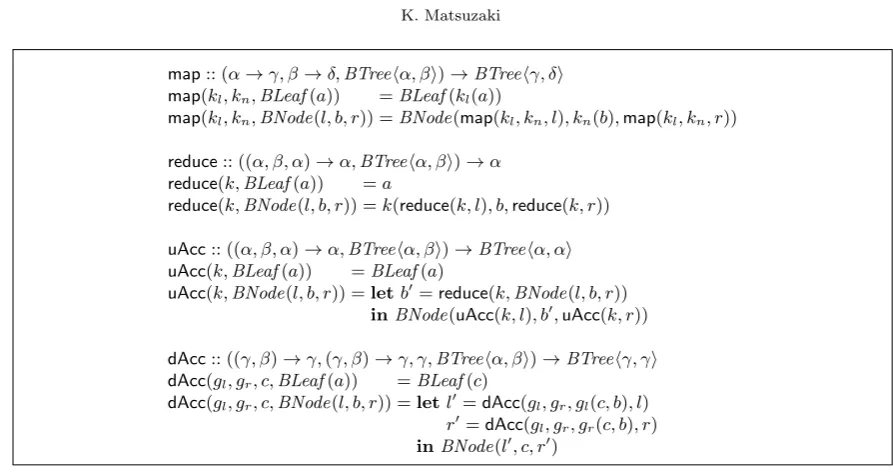
Fig. 3.1.An example ofm-critical nodes andm-bridges. Left: In this binary tree, there are three4-critical nodes denoted by
the doubly-lined circles. The number in each node denotes the number of nodes in the subtree. Right: For the same tree there are seven4-bridges, (a)–(g), each of which is a set of connected nodes.
It is worth noting that the set of auxiliary functions is not unique. For example, we can define another set of auxiliary functions in which an intermediate value has a flag and two values.
In general, auxiliary functions are more complicated than the original function as we have seen in this example. This complexity of auxiliary functions would introduce overheads in the derived parallel algorithms.
3. Division of Binary Trees with High Locality. To develop efficient parallel programs on distributed-memory parallel computers, we need to divide data into smaller parts and distribute them to the processors. Here, the division of data should have the following two properties for efficiency of parallel programs. The first property islocality. The data distributed to each processor should be adjacent. If two elements adjacent in the original data are distributed to different processors, then we often need communications between the processors. The second property is load balance. The number of elements distributed to each processor should be nearly equal since the cost of local computation is often proportional to the number of elements.
It is easy to divide a list with these two properties, that is, for a given list ofN elements we simply divide the list into P sublists each havingN/P elements. It is, however, difficult to divide a tree satisfying the two properties due to the nonlinear and irregular structure of binary trees.
In this section, we introduce a division of binary trees based on the basic graph theory [8, 30], and show how to represent the distributed tree structures for efficient implementation of tree skeletons.
3.1. Graph-Theoretic Results for Division of Binary Trees. We start by introducing some graph-theoretic results [8, 30]. Let size(v) denote the number of nodes in the subtree rooted at nodev.
Definition 3.1 (m-Critical Node). Let m be an integer. A nodev is called an m-critical node, if • v is an internal node, and
• for each child v′ of v inequality⌈size(v)/m⌉>⌈size(v′)/m⌉holds.
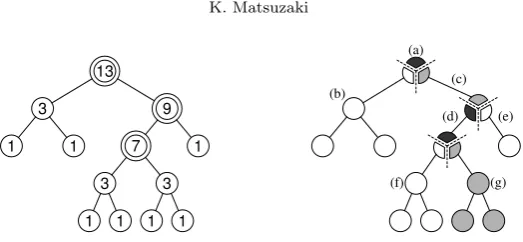
Them-critical nodes divide a tree into sets of adjacent nodes (m-bridges) as shown in Fig. 3.1.
Definition 3.2 (m-Bridge). Let m be an integer. An m-bridge is a set of adjacent nodes divided by m-critical nodes, that is, a largest set of adjacent nodes in whichm-critical nodes are only at the root or bottom.
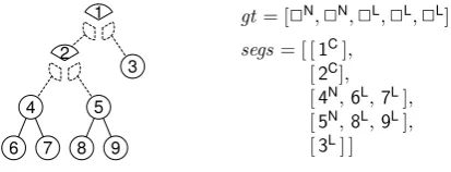
In the following of this paper, we assume that each local segment given by dividing a tree is anm-bridge. The global structure ofm-bridges also forms a binary tree.
Them-critical nodes and them-bridges have several important properties. The following two lemmas show properties of them-critical nodes and them-bridges in terms of the global shape of them.
Lemma 3.3. If v1 andv2arem-critical nodes then their least common ancestor is also anm-critical node.
Lemma 3.4. If B is anm-bridge of a tree then B has at most onem-critical node among the leaves of it. The root node in each m-bridge, except them-bridge that includes the global root node, is an m-critical node. If we remove the root m-critical node if it exists, it follows from Lemma 3.4 and Definition 3.2 that the
1
2 3
4 5
6 7 8 9
gt= [✷N,✷ N
,✷ L
,✷ L
,✷ L
]
segs= [ [1C],
[2C],
[4N ,6
L ,7
L], [5N
,8 L
,9 L
], [3L] ]
Fig. 3.2. Array representation of divided binary trees. Each local segment of segs is assigned to one of processors and is not shared. Labels L,Nand Cdenote a leaf, a normal internal node, and anm-critical node, respectively. Each m-critical node is
included in the parent segment.
The following three lemmas are related to the number of nodes in anm-bridge and the number ofm-bridges in a tree. Note that the first two lemmas hold on general trees while the last lemma only holds on binary trees.
Lemma 3.5. The number of nodes in anm-bridge is at mostm+ 1.
Lemma 3.6. Let N be the number of nodes in a tree then the number of m-critical nodes in the tree is at most 2N/m−1.
Lemma 3.7. Let N be the number of nodes in a binary tree then the number of m-critical nodes in the binary tree is at least (N/m−1)/2.
LetN be the number of nodes and P be the number of processors. In the previous studies [8, 18, 30], we divided a tree into m-bridges using the parameter m given bym = 2N/P. Under this division we obtain at most (2P−1)m-bridges and thus each processor handles at most twom-bridges. Of course this division enjoys high locality, but it has poor load balance since the maximum number of nodes passed to a processor may be 2N/P, which is twice of that for the best lead-balancing case.
In Sect. 5, we will adjust the value m for better division of binary trees based on the cost model of tree skeletons. The idea is to divide a binary tree into more m-bridges using smaller m so that we obtain enough load balance while keeping the overheads caused by loss of locality small.
3.2. Data Structure for Distributed Segments. The performance of the sequential computation parts is as important as that of the communication parts.
Generally speaking, tree structures are often implemented using pointers or references. There are, however, two problems in this implementation for large-scale tree applications. First, much memory is required for pointers. Considering trees of integers or real numbers, for example, we can see that the pointers use as much memory as the values do. Furthermore, if we allocate nodes one by one, more memory is consumed to enable each of them to be deallocated. Second, locality is often lost. Recent computers have a cache hierarchy to bridge the gap between the CPU speed and the memory speed, and cache misses greatly decrease the performance especially in data-intensive applications. If we allocate nodes from here and there then the probability of cache misses increases.
To resolve these problems, we represent a binary tree with arrays. We represent a tree divided by the
m-bridges using one array gt for the global structure and one array of arrays segs for the local segments, each of which is given by serializing the tree in the order of prefix traversal. Note that arrays in segs are distributed among processors, while each local segment exists in only one processor. Figure 3.2 illustrates the array representation of a distributed tree. Since adjoining elements are aligned one next to another in this representation, we can reduce cache misses.
Table 4.1
Parameters of the cost model.
tp(f) computational time of functionf usingpprocessors N the number of nodes in the input tree
P the number of processors
m the parameter form-critical nodes andm-bridges
M the number of segments given by division of trees
Li the number of nodes in theith segment
Di the depth of them-critical node in theith segment cα the time needed for communicating one data of typeα |α| the size of a value of typeα
4. Implementation and Cost Model of Tree Skeletons. In this section, we show an implementation and a cost model of the tree skeletons on distributed-memory parallel computers. We implement the local computation in tree skeletons using loops and stacks on the serialized arrays, which play an important role in reducing the cache misses and achieving high performance in the sequential computation parts.
We define several parameters for discussion of the cost model (Table 4.1). We assume a homogeneous distributed-memory environments as the computation environment. The computational time of function f
executed withpprocessors is denoted bytp(f). In particular,t1(f) denotes the cost of sequential computation
of f. Parameter N denotes the number of nodes, andP denotes the number of processors. Parameter m is used form-critical nodes andm-bridges, andM denotes the number of segments after the division. For theith segment, in addition to the parameter of the number of nodes Li, we introduce parameter Di indicating the
depth of the critical node. Parametercα denotes the communication time for a value of typeα. The size of a
value of type αis denoted by|α|.
The cost of tree skeletons can be uniformly given as the sum of the maximum local-computation cost and the global-computation cost as follows.
max
p ∑
pr(i)=p
(Li×tl+Di×td) +M×tm
In the expression of the cost,∑
pr(i)=pdenotes the summation of cost for local segments associated to processor
p. The parametertl indicates the cost of computation that is applied to each node in a segment, the parameter td indicates the cost of computation that is applied to the nodes on the path from the root to them-critical
node, and the parametertm denotes the communication cost required for each segment.
In fact, we can extend the implementation of tree skeletons and the cost model to the bulk-synchronous parallel (BSP) model [37]. The cost of a BSP algorithm is given by the sum of costs of supersteps, which consists of local computation followed by communication and barrier synchronization. The cost of a superstep is given by an expression of the form w+hg+l where wis the maximum cost of local computation, h is the size of messages,gis the cost of communicating a message of size one, andlis the cost of the barrier synchronization. Note that for the parameterg we havecα=|α|g for any typeα.
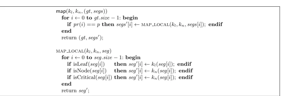
4.1. Map. Since there is no dependency among nodes in the computation of the map skeleton, we can implement the map skeleton by applying function map local to each local segment, where the map local
function applies functionklto each leaf and functionkn to each internal node and them-critical node in a local
segment. The implementation of themapskeleton is given in Fig. 4.1.
In a local segment withLinodes, the number of leaves is at mostLi/2 + 1 and the number of internal nodes
including the m-critical node is at mostLi/2 + 1. Ignoring small constants we can specify the computational
cost of themap localfunction as
t1(map local) = Li
2 ×t1(kl) +
Li
map(kl, kn,(gt,segs))
fori←0togt.size−1:begin
if pr(i) ==pthensegs′[i]←map local(k
l, kn,segs[i]); endif end
return (gt,segs′);
map local(kl, kn,seg)
fori←0toseg.size−1:begin
if isLeaf(seg[i]) thenseg′[i]←kl(seg[i]); endif if isNode(seg[i]) thenseg′[i]←k
n(seg[i]); endif if isCritical(seg[i])thenseg′[i]←kn(seg[i]); endif end
returnseg′;
Fig. 4.1. Implementation ofmapskeleton.
The cost of the mapskeleton is as follows.
tP(map(kl, kn, t)) = max p
∑
pr(i)=p
Li×
t1(kl) +t1(kn)
2
On the BSP model, we can implement the map skeleton with a single superstep without communication. Thus, the BSP cost is given as follows.
t⟨BSP⟩P (map(kl, kn, t)) = max p
∑
pr(i)=p Li×
t1(kl) +t1(kn)
2 +l
4.2. Reduce. We then show an implementation and its cost of the reduceskeleton called with functionk
and auxiliary functionsk=⟨φ, ψn, ψl, ψr⟩u. Let the input binary tree have typeBTree⟨α, β⟩and intermediate
values for auxiliary functions have type γ. The implementation of thereduce skeleton is shown in Fig. 4.2.
Step 1. Local Reduction. The bottom-up computation of the reduce skeleton can be computed by a traversal on the array from right to left using a stack for the intermediate results. Firstly we apply
reduce localfunction to each local segment to reduce it to a value. In thereduce localfunction, • we apply functionsφand eitherψl orψrto them-critical node and its ancestors, and
• we apply functionkto the other internal nodes.
Here, applying the functionkis cheaper than applying functionφandψn, even thoughk(l, n, r) =ψn(l, φ(n), r)
holds with respect to the results of functions. To specify where the m-critical node or its ancestor is in the stack, we use a variable d that indicates the position. Note that in the computation of the reduce local
function, at most one element in the stack has the value of the m-critical node or its ancestors.
In this step, functionsφand eitherψlorψrare applied to them-critical node and its ancestors (Dinodes)
and function kis applied to the other internal nodes ((Mi/2−Di) nodes). Thus, the cost ofreduce localis
given as follows.
t1(reduce local) =Di×(t1(φ) + max(t1(ψl), t1(ψr))) +
(L
i
2 −Di
) ×t1(k)
Step 2. Gathering Local Results to Root Processor. In the second step, we gather the local results to the root processor. The communication cost is given by the number of leaf segments of type α and the number of internal segments of typeγ.
tP(Step 2) = M
2 ×cα+
M
2 ×cγ
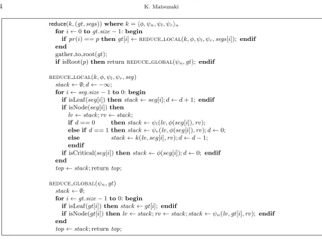
reduce(k,(gt,segs))wherek=⟨φ, ψn, ψl, ψr⟩u fori←0togt.size−1:begin
if pr(i) ==pthengt[i]←reduce local(k, φ, ψl, ψr,segs[i]); endif end
gather to root(gt);
if isRoot(p)thenreturnreduce global(ψn,gt); endif
reduce local(k, φ, ψl, ψr,seg) stack← ∅;d← −∞;
fori←seg.size−1to0:begin
if isLeaf(seg[i])thenstack←seg[i];d←d+ 1; endif if isNode(seg[i])then
lv←stack;rv←stack;
if d== 0 thenstack←ψl(lv, φ(seg[i]),rv); else if d== 1thenstack←ψr(lv, φ(seg[i]),rv);d←0; else stack←k(lv, seg[i],rv);d←d−1;
endif
if isCritical(seg[i])thenstack ←φ(seg[i]);d←0; endif end
top←stack; returntop;
reduce global(ψn,gt) stack← ∅;
fori←gt.size−1to0:begin
if isLeaf(gt[i])thenstack←gt[i]; endif
if isNode(gt[i])thenlv←stack;rv←stack;stack←ψn(lv,gt[i],rv); endif end
top←stack; returntop;
Fig. 4.2.Implementation ofreduceskeleton
Step 3. Global Reduction on Root Processor. Finally, we compute the result of thereduce skeleton by applying thereduce global function to the array of local results. This computation is performed on the root processor. We compute the result by applyingψn for each internal node in a bottom-up manner, which is
implemented by a traversal with a stack on the array of the global structure from right to left.
In this step the functionψn is applied to each internal segment and the cost ofreduce globalis
t1(reduce global) = M
2 ×t1(ψn).
In summary, the cost of the reduceskeleton is given as follows.
tP(reducek)
= max
p ∑
pr(i)=p
t1(reduce local) +tP(Step 2) +t1(reduce global)
= max
p ∑
pr(i)=p
( Li×
t1(k)
2 +Di×(−t1(k) +t1(φ) + max(t1(ψl), t1(ψr)))
)
+M ×cα+cγ2+t1(ψn)
2; the other consists of Step 3. Thus, the BSP cost is given as follows.
t⟨BSP⟩P (reducek) = max
p ∑
pr(i)=p
( Li×
t1(k)
2 +Di×(−t1(k) +t1(φ) + max(t1(ψl), t1(ψr)))
)
+M ×t1(ψn)/2 +M×| α|+|γ|
2 ×g+ 2l
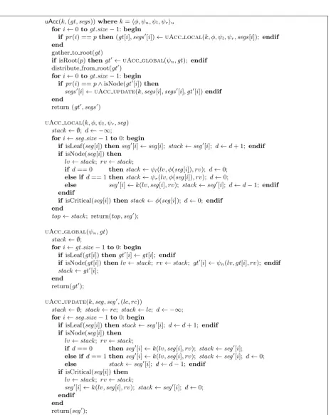
4.3. Upwards Accumulate. Next, we develop an implementation of theuAccskeleton called with func-tionk and auxiliary functionsk=⟨φ, ψn, ψl, ψr⟩u. Similar to the reduceskeleton, let the type of input binary
tree beBTree⟨α, β⟩and the type of intermediate values beγ. The implementation of theuAccskeleton is shown in Fig. 4.3.
Step 1. Local Upwards Accumulation. In the first step, we apply function uAcc local to each segment and compute local upwards accumulation and reduction. This function puts the intermediate results to arrayseg′ if a node has no m-critical node as descendants, since the result value is indeed the result of the uAccskeleton. This function puts nothing to arrayseg′ if a node is either them-critical node or an ancestor of them-critical node. Returned values are the result of local reduction and the arrayseg′.
In the computation of theuAcc local function,φand either ofψl orψr are applied to each node of the m-critical node and its ancestors (Di nodes), andkis applied to the other internal nodes ((Li/2−Di) nodes).
We obtain the cost of theuAcc localfunction as
t1(uAcc local) =Di×(t1(φ) + max(t1(ψl), t1(ψr))) +
(L
i
2 −Di
)
×t1(k).
Note that this cost is the same as that of reduce localfunction.
Step 2. Gathering Results of Local Reductions to Root Processor. In the second step, we gather the results of the local reductions on the global structure gt of the root processor. From each leaf segment a value of type α is transferred, and from each internal segment a value of type γ is transferred. Since the number of leaf segments and the number of internal segments are M/2 respectively, the communication cost of the second step is
tP(Step 2) = M
2 ×cα+
M
2 ×cγ .
Step 3. Global Upward Accumulation on Root Processor. In the third step, we compute the upwards accumulation for the global structure gt on the root processor. Function uAcc global performs sequential upwards accumulation using function ψn. In uAcc global, we apply functionψn to each internal
segment ofgt, and the cost of the third step is given as
t1(uAcc global) =M
2 ×t1(ψn).
Step 4. Distributing Global Result. In the fourth step, we send the result of global upwards accu-mulation to processors, where two values are sent to each internal segment and no values are sent to each leaf segment. Since all the values have type αafter the global upwards accumulation, the communication cost of the fourth step is given as
tP(Step 4) =M×cα.
Step 5. Local Updates for Each Internal Segment. In the last step, we apply functionuAcc update
to each internal segment. At the beginning of the function, the two values pushed in the previous step are pushed to the stack. These two values correspond to the results of children of them-critical node. Note that in the last step we only compute the missing values in the segmentseg′, which is given in the local upwards accumulation
uAcc(k,(gt,segs))wherek=⟨φ, ψn, ψl, ψr⟩u fori←0togt.size−1:begin
if pr(i) ==pthen(gt[i],segs′[i])←uAcc local(k, φ, ψl, ψr,segs[i]); endif end
gather to root(gt)
if isRoot(p)thengt′←uAcc global(ψ
n,gt); endif
distribute from root(gt′) fori←0togt.size−1:begin
if pr(i) ==p∧isNode(gt′[i])then
segs′[i]←uAcc update(k,segs[i],segs′[i],gt′[i])endif end
return (gt′,segs′)
uAcc local(k, φ, ψl, ψr,seg) stack ← ∅; d← −∞;
fori←seg.size−1to0:begin
if isLeaf(seg[i])thenseg′[i]←seg[i]; stack←seg′[i]; d←d+ 1; endif if isNode(seg[i])then
lv←stack; rv←stack;
if d== 0 thenstack←ψl(lv, φ(seg[i]), rv); d←0; else if d== 1thenstack←ψr(lv, φ(seg[i]), rv); d←0;
else seg′[i]←k(lv,seg[i], rv); stack←seg′[i]; d←d−1; endif endif
if isCritical(seg[i])thenstack←φ(seg[i]); d←0; endif end
top←stack; return(top,seg′);
uAcc global(ψn,gt) stack ← ∅;
fori←gt.size−1to0:begin
if isLeaf(gt[i])thengt′[i]←gt[i]; endif
if isNode(gt[i])thenlv←stack; rv←stack; gt′[i]
←ψn(lv, gt[i], rv); endif stack←gt′[i];
end
return(gt′);
uAcc update(k,seg,seg′,(lc, rc))
stack ← ∅; stack←rc; stack ←lc; d← −∞;
fori←seg.size−1to0:begin
if isLeaf(seg[i])thenstack ←seg′[i]; d←d+ 1; endif if isNode(seg[i])then
lv←stack; rv←stack;
if d== 0 thenseg′[i]←k(lv,seg[i], rv); stack←seg′[i]; else if d== 1thenseg′[i]←k(lv,seg[i], rv); stack←seg′[i]; d←0;
else stack←seg′[i]; d←d−1; endif if isCritical(seg[i])then
lv←stack; rv←stack;
seg′[i]
←k(lv,seg[i], rv); stack←seg′[i]; d ←0;
endif end
return(seg′);
In this step, functionkis applied to the nodes on the path from them-critical node to the root node for each internal segment. Noting that the depth of them-critical nodes isDi, we can give the cost ofuAcc updateas
t1(uAcc update) =Di×t1(k).
In summary, using the functions defined so far, we can implement theuAccskeleton. The cost of theuAcc
skeleton is given as follows.
tP(uAcc(k, t))
= max
p ∑
pr(i)=p
t1(uAcc local) +tP(Step 2) +t1(uAcc global)
+tP(Step 4) + max p
∑
pr(i)=p
t1(uAcc update)
= max
p ∑
pr(i)=p (
Li× t1(k)
2 +Di×(t1(φ) + max(t1(ψl), t1(ψr)))
)
+M×(3cα+cγ+t1(ψn))/2
On the BSP model, we can implement the uAccskeleton with three supersteps: the first one consists of Steps 1 and 2; the second one consists of Steps 3 and 4; the last one consists of Step 5. Thus, the BSP cost is given as follows.
t⟨BSP⟩P (uAcck) = max
p ∑
pr(i)=p
( Li×
t1(k)
2 +Di×(t1(φ) + max(t1(ψl), t1(ψr)))
)
+M×t1(ψn)/2 +M ×(3|α|+|γ|)/2×g+ 3l
4.4. Downwards Accumulate. Finally, we develop an implementation and the cost of thedAccskeleton called with a pair of functions (gl, gr) and auxiliary functions (gl, gr) =⟨φl, φr, ψu, ψd⟩d. Let the input binary
tree have typeBTree⟨α, β⟩, the accumulative parameterchave typeγ, and the intermediate values for auxiliary functions have typeδ. The implementation of thedAccskeleton is shown in Fig. 4.4.
Step 1. Computing Local Intermediate Values. In the first step, we compute for each internal segment two local intermediate values, which are used in updating the accumulative parameter from the root node to the both children of them-critical node. To minimize the computation cost, we first find them-critical node and then compute two values only on the path from the root node to them-critical node. We implement this computation by functiondAcc path, in which the computation is done by a traversal on the array from right to left with an integerdinstead of a stack. Two variablestoLandtoR are the intermediate values.
In this step we apply ψu twice and either φl or φr for each of the ancestors of the m-critical nodes (Di
nodes). Omitting some small constants, the cost of thedAcc pathfunction is given as
t1(dAcc path) =Di×(max(t1(φl), t1(φr)) + 2t1(ψu)).
Step 2. Gathering Local Results to Root Processor. In the second step, we gather the local results of the internal segments to the root processor. Since the two intermediate values have type δand the number of internal segments isM/2, the communication cost in the second step is given as
tP(Step 2) =M×cδ .
The pair of local results from each internal segment is put to the array of the global tree structuregt.
accumulative parameter in the stack is updated with the pair of local results given in the previous step. The result of global accumulation is the accumulative parameter passed to the root node for each segment.
The dAcc global function applies function ψd twice for each internal segment in the global structure.
The computational cost of thedAcc globalfunction is
t1(dAcc global) =M ×t1(ψd).
Step 4. Distributing Global Result. In the fourth step, we distribute the result of global downwards accumulation to the corresponding processor. Since each result of global downwards accumulation has type γ, the communication cost of the fourth step is
tP(step 4) =M×cγ .
Step 5. Local Downwards Accumulation. Finally, we compute local downwards accumulation for each segment. The initial value c′ of the accumulative parameter is given in the previous step. Note that the definition of dAcc localfunction is just the same as the sequential version of the downwards accumulation on the serialized array if we assume them-critical node as a leaf.
The local downwards accumulation applies functionsglandgrfor each internal node. Since the number of
the internal nodes isLi/2, the computational cost of thedAcc localfunction is given as t1(dAcc local) = Li
2 ×(t1(gl) +t1(gr)).
Summarizing the discussion so far, the cost of thedAccskeleton is given as follows.
tP(dAcc)
= max
p ∑
pr(i)=p
t1(dAcc path) +tP(Step 2) +t1(dAcc global)
+tP(Step 4) + max p
∑
pr(i)=p
t1(dAcc local)
= max
p ∑
pr(i)=p
( Li×
t1(gl) +t1(gr)
2 +Di×(max(t1(φl), t1(φr)) + 2t1(ψu))
)
+M×(cδ+t1(ψd) +cγ)
On the BSP model, we can implement the dAccskeleton with three supersteps: the first one consists of Steps 1 and 2; the second one consists of Steps 3 and 4; the last one consists of Step 5. Thus, the BSP cost is given as follows.
t⟨BSP⟩P (dAcc) = max
p ∑
pr(i)=p
( Li×
t1(gl) +t1(gr)
2 +Di×(max(t1(φl), t1(φr)) + 2t1(ψu))
)
+M×t1(ψd) +M×(|δ|+|γ|)×g+ 3l
5. Optimal Division of Binary Trees Based on Cost Model. As we stated at the beginning of Sect. 3, locality and load balance are two important issues in developing efficient parallel programs in particular on distributed-memory parallel computers. When we divide and distribute a binary tree using them-bridges, we enjoy good locality with largemwhile we enjoy good load balance with smallm. Therefore, we need to find an appropriate value formto achieve both good locality and good load balance.
First, we show relations among parameters of the cost model. From Lemma 3.5 and the representation of local segments in Fig. 3.2, we have
Li≤m .
dAcc(gl, gr, c,(gt,segs))where(gl, gr) =⟨φl, φr, ψu, ψd⟩d fori←0togt.size−1:begin
if pr(i) ==p∧isNode(gt[i])then
gt[i]←dAcc path(φl, φr, ψu,segs[i]); endif end
gather to root(gt)
if isRoot(p)thengt′←dAcc global(ψd, c,gt); endif
distribute from root(gt′) fori←0togt.size−1:begin
if pr(i) ==pthensegs′[i]←dAcc local(gl, gr,gt′[i],segs[i]); endif end
return (gt′,segs′)
dAcc path(φl, φr, ψu,seg) d← −∞;
fori←seg.size−1to0:begin
if isLeaf(seg[i])thend←d+ 1; endif if isNode(seg[i])then
if d== 0then
toL←ψu(φl(seg[i]),toL);toR←ψu(φl(seg[i]),toR); else if d== 1then
toL←ψu(φr(seg[i]),toL);toR←ψu(φr(seg[i]),toR); d←0; else
d←d−1;
endif endif
if isCritical(seg[i])thentoL←φl(seg[i]);toR←φr(seg[i]); d←0; endif end
return (toL,toR);
dAcc global(ψd, c,gt) stack← ∅;stack←c;
fori←0togt.size−1:begin
if isLeaf(gt[i])thengt′[i]←stack; endif if isNode(gt[i])then
gt′[i]
←stack; (toL,toR)←gt[i];
stack←ψd(gt′[i],toR);stack←ψd(gt′[i],toL); endif
end
returngt′;
dAcc local(gl, gr, c′,seg) stack← ∅;stack←c′;
fori←0toseg.size−1:begin
if isLeaf(seg[i])thenseg′[i]←stack; endif if isNode(seg[i])then
seg′[i]←stack;stack←g
r(seg′[i],seg[i]);stack ←gl(seg′[i],seg[i]); endif if isCritical(seg[i])thenseg′[i]←stack; endif
end
returnseg′;
Since the height of a tree is at least a half of the number of nodes, we obtain
Di≤Li/2≤m/2 .
(5.2)
From Lemmas 3.6 and 3.7, the number of local segments M is bound with the number N of nodes and the parameter mas follows.
1 2
(N
m−1 )
≤M ≤ 2mN −1 (5.3)
By inequality (5.2), the general form of the cost can be transformed into the following simpler form by considering the worst case.
max
p ∑
pr(i)=p
(Li×tl+Di×td) +M×tm≤(max p
∑
pr(i)=p
Li)× (
tl+ td
2
)
+M×tm
We then bound the maximum number of nodes on a processor, maxp∑pr(i)=pLi. We distribute the local segment to processors so as to obtain good load balance, and one easy way to implement the load balancing is greedy distribution of the local segments from the largest one. By this greedy distribution, the difference between the maximum number of nodes maxp∑pr(i)=pLiand the minimum number of nodes minp
∑
pr(i)=pLi is less than or equal to the maximum number of nodes in a segment. Since the maximum number of nodes in a local segment is mas stated in inequality (5.1) and the total number of nodes in the original binary tree isN, we can bound the maximum number of nodes distributed to a processor as follows:
max
p ∑
pr(i)=p
Li ≤ N P +m
where P denotes the number of processors. By substituting this inequality to the cost, we can bound the cost of the worst case.
max
p ∑
pr(i)=p
(Li×tl+Di×td) +M ×tm≤
(N
P +m )
× (
tl+ td
2
)
+M×tm
(5.4)
Now we want to minimize the worst-case cost given in the right-hand side of inequality (5.4). By substituting the parameterM(inequality (5.3)), the worst-case cost is bound with respect tom. We can bound the worst-case cost for smaller mas
( N P +m
) ×
( tl+
td
2
)
+M×tm≤ (
N P +m
) ×
( tl+
td 2 ) +1 2 ( N m−1
) ×tm,
and we can bound the worst-case cost for larger mas
( N P +m
) ×
( tl+
td
2
)
+M×tm≤ (
N P +m
) ×
( tl+
td
2
)
+2N
m −1×tm .
From these bounds, we can minimize the worst-case cost for some valuemin the following range.
√ tm
2tl+td √
N ≤m≤2
√ tm
2tl+td √
N
(5.5)
0 0.05 0.1 0.15 0.2
1 4 6 8 12 16 24 32
Time (s)
Number of Processors Balanced Ill-Balanced Random
0 5 10 15 20 25 30
1 4 6 8 12 16 24 32
Speedup
Number of Processors Balanced
Ill-Balanced Random
Fig. 6.1. For the sum of node values, execution times and speedups against sequential program plotted to the number of processors. The parametermfor the division of trees ism= 53,600.
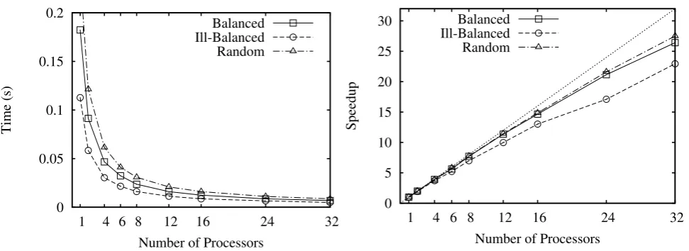
6. Experiment Results. To confirm the efficiency of the implementation algorithm for binary-tree skele-tons, we implemented binary tree skeletons in C++ and MPI and made several experiments. We used our PC-cluster of uniform PCs with two Pentium 4 2.4-GHz CPUs (one CPU is used for each PC) and 2-GByte memory connected with Gigabit Ethernet. The compiler and MPI library used are gcc 4.1.1 and MPICH 1.2.7, respectively.
We used the skeletal parallel programs of the two examples in Sect. 2. The input trees are (1) a balanced tree, (2) a randomly generated tree and (3) a fully ill-balanced tree, each having 16,777,215 (= 224−1) nodes.
Figures 6.1 and 6.2 show the general performance of tree skeletons. Each execution time excludes the initial data distribution and final gathering. The speedups are plotted against the efficient sequential implementation of the program, which is implemented on the array representing binary trees based on the same sequential algorithm. As seen in these plots, our implementation shows good scalability even against the efficient sequential programs. By the m-bridges, the balanced tree is divided into leaf segments of the same size and internal segments consisting only of one node. Therefore, the overhead caused by parallelism is very small for the balanced binary tree, and the implementation achieves almost linear speedups against the sequential program. For the random tree, the average depth of the m-critical nodes is so small that the implementation achieves good performance close to that for the balance tree. The fully ill-balanced tree, however, is divided into leaf segments consisting of one node and internal segments with theirm-critical node at the depthDi =Li/2. From
the cost model and its parameters, the skeletal parallel program has overheads caused by the factor of depth of the m-critical nodes. In fact, the experimental results show that the skeletal parallel program runs slower for the fully ill-balanced tree than for the other two inputs.
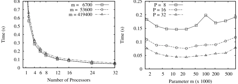
To analyze the cost model and the range of the parameter mmore in detail, we made more experiments for the randomly generated tree by changing the value of the parameterm. We measured the parameterstl,td,
and tm of the cost model with a small tree with 999,999 nodes, and estimated the value of them astl= 0.057 µs, td = 0.03 µs, andtm = 71 µs. By substituting the parameters, we can expect good performance of the
skeletal program under the range 90,000 < m < 180,000. Figure 6.3 (left) plots the execution times to the number of processors for three values of the parameterm. As we can see from this figure, the implementation achieves good performance for a wide range ofm. Figure 6.3 (right) plots the execution times to the parameter
m. This figure shows that the performance gets worse if the parameter m is too small (m < 5,000) or too large (m > 200,000). For the parameter m in the range above the skeletal program achieves near the best performance, and we conclude that the cost model and the estimation of the parametermis useful for efficient implementations.
0 0.2 0.4 0.6 0.8 1 1.2
1 4 6 8 12 16 24 32
Time (s)
Number of Processors Balanced Ill-Balanced Random
0 5 10 15 20 25 30
1 4 6 8 12 16 24 32
Speedup
Number of Processors Balanced
Ill-Balanced Random
Fig. 6.2. For the prefix numbering problem, execution times and speedups against sequential program plotted to the number of processors. The parametermfor the division of trees ism= 53,600.
0 0.1 0.2 0.3 0.4 0.5 0.6 0.7 0.8
1 4 6 8 12 16 24 32
Time (s)
Number of Processors m = 6700 m = 53600 m = 419400
0 0.05 0.1 0.15 0.2 0.25
2 5 10 20 50 100 200 500
Time (s)
Parameter m (x 1000) P = 8
P = 16 P = 32
Fig. 6.3.For the prefix numbering problem, execution times plotted to the number of processors and to the parameterm. The
input trees are from the same randomly generated tree divided with different parameterm.
to developing efficient implementations of tree contraction algorithms on various parallel models [1, 2, 3, 4, 5, 9, 13, 23, 24, 38]. Among them, Gibbons and Rytter developed a cost-optimal algorithm on CREW PRAM [9]; Abrahamson et al. developed a cost-optimal and practical algorithm on EREW PRAM [1]; Miller and Reif showed implementations on hypercubes or related networks [23, 24]; and recently more efficient implementations are discussed [2, 38] for symmetric multiprocessors (SMP) and chip-level multiprocessing (CMP). A lot of tree programs have been described by the tree contraction algorithms [3, 4, 9, 12, 17, 26, 27, 28, 29].
In terms of manipulations of general trees, which are formalized as parallel rose-tree skeletons [20], some of them are implemented efficiently in parallel [15, 32]. Sevilgen et al. [32] has shown an implementation algorithm for tree accumulations on general trees where rather strict conditions are requested for efficient implementation. Kakehi et al. [14] has developed an efficient implementation of tree reduction on general trees based on the serialized representation like XML formats.
8. Conclusion. In this paper, we have developed an efficient implementation of parallel tree skeletons. Not only our implementation shows good performance even against sequential programs, but also the cost model of the implementation helps us to divide a tree into segments with good load balance. The implementation is available as part of SkeTo library (http://sketo.ipl-lab.org/). One of our future work is to develop a profiling system to determine the parametermmore accurately.
REFERENCES
[1] K. R. Abrahamson, N. Dadoun, D. G. Kirkpatrick, and T. M. Przytycka,A simple parallel tree contraction algorithm, J. Algorithm., 10 (1989), pp. 287–302.
[2] D. A. Bader, S. Sreshta, and N. R. Weisse-Bernstein,Evaluating arithmetic expressions using tree contraction: A fast and scalable parallel implementation for symmetric multiprocessors (SMPs) (extended abstract), in Proceedings of 9th International Conference on High Performance Computing (HiPC 2002), Springer, 2002, pp. 63–78.
[3] R. P. K. Banerjee, V. Goel, and A. Mukherjee,Efficient parallel evaluation of CSG tree using fixed number of processors, in ACM Symposium on Solid Modeling Foundations and CAD/CAM Applications, May 19–21, 1993, Montreal, Canada, 1993, pp. 137–146.
[4] R. Cole and U. Vishkin,The accelerated centroid decomposition technique for optimal parallel tree evaluation in logarithmic time, Algorithmica, 3 (1988), pp. 329–346.
[5] F. K. H. A. Dehne, A. Ferreira, E. C´aceres, S. W. Song, and A. Roncato, Efficient parallel graph algorithms for coarse-grained multicomputers and BSP, Algorithmica, 33 (2002), pp. 183–200.
[6] H. Deldari, J. R. Davy, and P. M. Dew,Parallel CSG, skeletons and performance modeling, in Proceedings of the Second Annual CSI Computer Conference (CSICC’96), 1996, pp. 115–122.
[7] K. Diks and T. Hagerup, More general parallel tree contraction: Register allocation and broadcasting in a tree, Theor. Comput. Sci., 203 (1998), pp. 3–29.
[8] H. Gazit, G. L. Miller, and S.-H. Teng, Optimal tree contraction in EREW model, in Proceedings of the Princeton Workshop on Algorithms, Architectures, and Technical Issues for Models of Concurrent Computation, 1987, pp. 139–156. [9] A. Gibbons and W. Rytter, An optimal parallel algorithm for dynamic expression evaluation and its applications, in Proceedings of the 6th Conference on Foundations of Software Technology and Theoretical Computer Science, Springer, 1986, pp. 453–469.
[10] J. Gibbons,Computing downwards accumulations on trees quickly, in Proceedings of the 16th Australian Computer Science Conference, 1993, pp. 685–691.
[11] J. Gibbons, W. Cai, and D. B. Skillicorn,Efficient parallel algorithms for tree accumulations, Sci. Comput. Program., 23 (1994), pp. 1–18.
[12] X. He,Efficient parallel algorithms for solving some tree problems, in 24th Allerton Conference on Communication, Control and Computing, 1986, pp. 777–786.
[13] G. Jens,Communication and memory optimized tree contraction and list ranking, Tech. report, INRIA, Unit´e de recherche, Rhˆone-Alpes, Montbonnot-Saint-Martin, FRANCE, 2000.
[14] K. Kakehi, K. Matsuzaki, and K. Emoto,Efficient parallel tree reductions on distributed memory environments, in Pro-ceedings of the 7th International Conference on Computational Science (ICCS 2007), Part II, Springer, 2007, pp. 601–608. [15] K. Kakehi, K. Matsuzaki, K. Emoto, and Z. Hu,An practicable framework for tree reductions under distributed memory environments, Tech. Report METR 2006-64, Department of Mathematical Informatics, Graduate School of Information Science and Technology, the University of Tokyo, 2006.
[16] K. Matsuzaki,Efficient implementation of tree accumulations on distributed-memory parallel computers, in Proceedings of the 7th International Conference on Computational Science (ICCS 2007), Part II, Springer, 2007, pp. 609–616.
[17] K. Matsuzaki, Z. Hu, K. Kakehi, and M. Takeichi,Systematic derivation of tree contraction algorithms, Parallel Process. Lett., 15 (2005), pp. 321–336.
[18] K. Matsuzaki, Z. Hu, and M. Takeichi,Implementation of parallel tree skeletons on distributed systems, in Proceedings of The Third Asian Workshop on Programming Languages and Systems (APLAS’02), 2002, pp. 258–271.
[19] , Parallelization with tree skeletons, in Proceedings of the 9th International Euro-Par Conference (Euro-Par 2003), Springer, 2003, pp. 789–798.
[20] ,Parallel skeletons for manipulating general trees, Parallel Comput., 32 (2006), pp. 590–603.
[21] , Towards automatic parallelization of tree reductions in dynamic programming, in Proceedings of the 18th Annual ACM Symposium on Parallelism in Algorithms and Architectures (SPAA 2006), ACM Press, 2006, pp. 39–48.
[23] E. W. Mayr and R. Werchner,Optimal routing of parentheses on the hypercube, J. Parallel Dist. Com., 26 (1995), pp. 181– 192.
[24] ,Optimal tree contraction and term matching on the hypercube and related networks, Algorithmica, 18 (1997), pp. 445– 460.
[25] G. L. Miller and J. H. Reif,Parallel tree contraction and its application, in Proceedings of 26th Annual Symposium on Foundations of Computer Science, IEEE Computer Society, 1985, pp. 478–489.
[26] ,Parallel tree contraction, part 2: Further applications, SIAM J. Comput., 20 (1991), pp. 1128–1147.
[27] G. L. Miller and S.-H. Teng,Dynamic parallel complexity of computational circuits, in Proceedings of the Nineteenth Annual ACM Symposium on Theory of Computing, ACM Press, 1987, pp. 254–263.
[28] ,Tree-based parallel algorithm design, Algorithmica, 19 (1997), pp. 369–389.
[29] ,The dynamic parallel complexity of computational circuits, SIAM J. Comput., 28 (1999), pp. 1664–1688. [30] J. H. Reif, ed.,Synthesis of Parallel Algorithms, Morgan Kaufmann Publishers, February 1993.
[31] S. Sato and K. Matsuzaki,A generic implementation of tree skeletons, International Journal of Parallel Programming, 44 (2016), pp. 686–707.
[32] F. E. Sevilgen, S. Aluru, and N. Futamura,Parallel algorithms for tree accumulations, J. Parallel Dist. Com., 65 (2005), pp. 85–93.
[33] D. B. Skillicorn,Foundations of Parallel Programming, vol. 6 of Cambridge International Series on Parallel Computation, Cambridge University Press, 1994.
[34] ,Parallel implementation of tree skeletons, J. Parallel Dist. Com., 39 (1996), pp. 115–125. [35] ,A parallel tree difference algorithm, Inform. Process. Lett., 60 (1996), pp. 231–235.
[36] ,Structured parallel computation in structured documents, J. Univars. Comput. Sci., 3 (1997), pp. 42–68.
[37] D. B. Skillicorn, J. M. D. Hill, and W. F. McColl,Questions and Answers about BSP, Scientific Programming, 6 (1997), pp. 249–274.
[38] U. Vishkin,A no-busy-wait balanced tree parallel algorithmic paradigm, in Proceedings of the 12th Annual ACM Symposium on Parallel Algorithms and Architectures (SPAA 2000), ACM Press, 2000, pp. 147–155.