Interval Estimation of the Availability of a Two-Compressor with Erlangian Repair Time

(1)

Interval Estimation of the Availability of a

Two-Compressor with Erlangian Repair Time

Mohamed S. EL-Sherbeny1,2,*, Zienab M. Hussien1 1

Department of Mathematics, Faculty of Science & Arts, Rabigh- King AbdullAziz University, Rabigh, Saudi Arabia 2

Department of Mathematics, Faculty of Science, Helwan University, Cairo, Egypt

Abstract

This paper presents the reliability analysis of a two-compressor (non-identical) parallel system, which is part of the refrigeration system serving an ammonia storage tank. The failure rate of any compressor is a constant and the repair time distribution is a two-stage Erlanglan distribution. Measures of system performance such as reliability, system availability, and steady-state availability are derived. Also, a consistent asymptotically normal estimator and an asymptotic confidence interval for the steady-state availability and the mean time to failure of this system are obtained. Finally, a numerical example illustrates the results.

Keywords

Mean time to system failure, Steady-state availability, Erlang distribution

1. Introduction

Recent technological developments have given rise to the design of many complex systems containing several subsystems to perform different operations in various fields such as defence, industry and engineering systems. Because of the varied nature, these problems have attracted the attention of systems engineers and applied probabilists.

Repairable systems were studied in the past with reference to the evaluation of their performance in terms of reliability and availability. Work (Claasen, S.J., Joubert & Yadavalli) [2] have considered a two-unit standby system with non-instantaneous switch-over and "dead time" and obtain exact confidence limits for the steady-state availability of system. In the work (Chandrasekhar, Natarajan & Yadavalli) [1] studied the two unit standby system and obtain exact confidence limits for the steady-state availability of system, when the failure rate of an operative unit is constant and the repair time of the failed unit follows a two stage Erlang distribution. The stochastic analysis of a non-identical two-unit parallel system with common-cause failure by graphical evaluation and review technique (GERT) considered by (Sridharan & Kalyani) [6]. The cost-benefit analysis of a two-unit cold standby system with two types of repair- minor (regular) and major (expert) are considered by [5, 9] studied the optimal system for series systems with

* Corresponding author:

[email protected] (Mohamed S. EL-Sherbeny) Published online at http://journal.sapub.org/am

Copyright©2018The Author(s).PublishedbyScientific&AcademicPublishing This work is licensed under the Creative Commons Attribution International License (CC BY). http://creativecommons.org/licenses/by/4.0/

mixed standby components. In the work (Wang, Liu & Pearn) [4] studied the availability analysis of three different series system configurations with warm standby components and general repair times. Work (Wang & Kuo) [3] has considered the reliability and availability characteristics of four different series system configurations with mixed standby.

The purpose of the present paper is to study reliability analysis of a two-compressor arranging in parallel and find an estimator and asymptotic confidence interval for steady-state availability and mean time to failure of the system.

2. Description of the System

(2)

repairing process of the compressor is started but it doesn’t complete, while the repairing process is completed in the second stage. Each compressor is assumed to be as new after repairment.

Since an Erlang distribution can be considered as the distribution of the sum of two independent and identically distributed exponential random variables, the stochastic

process describing the behavior of the system is a Markov Process.

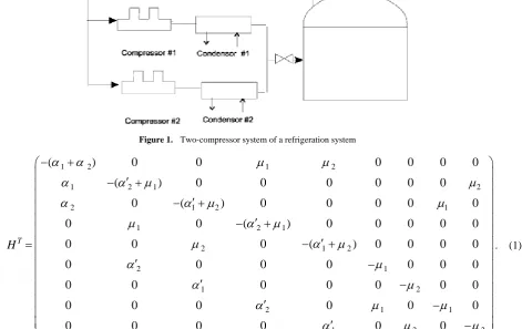
Let P t_i( ), i=0,..,8 be the probability that the system is in state S_i at time

t

. The infinitesimal generator of the Markov Process is given below.

Figure 1. Two-compressor system of a refrigeration system

1 2 1 2

2 1 2 1

1 2 1

2 1 2

2 1

1 2

2 1 1

1 2 2

( ) 0 0 0 0 0 0

0 ( ) 0 0 0 0 0

0 0 ( ) 0 0 0 0 0

0 0 0 ( ) 0 0 0 0

0 0 0 0 0 0 0

0 0 0 0 0 0

− +

 

 

′

− +

 

 ₋ _′₊ 

 

 ₋ _′ ₊ 

 

′

 − + 

=

 

′ −

 

 _′ ₋ 

 

 _′ ₋ 

 

 _′ ₋ 

 

T

H

α

µ

α

µ

α

µ

α

µ

α

µ

α

µ

α

µ

α

µ

α

µ

. (1)

We assume that initially both the compressors are operable and obtain the measures of system performance.

3. System Availability

The system availability is the probability that the system operates within the tolerances at a given instant of time and is obtained as follows. Include the diagram for the infinitesimal generator for the system of ODEs for probabilities P t_i′( ); eq. (1) and eqs. (2) to (10).

0′( )= −( 1+ 2) 0( )+ 1 3( )+ 2 4( ),

P t

α

P t

µ

P t

µ

P t (2)

1′( )= −( 2′ + 1) ( )1 + 1 0( )+ 2 8( ),

P t α µ P t α P t µ P t (3)

2′( )= −( 1′+ 2) 2( )+ 2 0( )+ 1 7( ),

P t

α

µ

P t

α

P t

µ

P t (4)

3′( )= −( 2′ + 1) 3( )+ 1 1( ),

P t

α

µ

P t

µ

P t (5)

4′( )= −( 1′+ 2) 4( )+ 2 2( ),

P t α µ P t µ P t (6)

5′( )= − 1 5( )+ 2′ 1( ),

P t µP t α P t (7)

6′( )= − 2 6( )+ 1 2′ ( ),

P t

µ

P t

α

P t (8)

7′( )= − 1 7( )+ 2 3′ ( )+ 1 5( ),

(3)

8′( )= − 2 8( )+ 1 4′ ( )+ 2 6( ).

P t

µ

P t

α

P t

µ

P t (10) At time t=0,P₀(0)=1 and all the other initial condition probabilities are equal to zero.

Taking Laplace transforms on both the sides of the differential equations given above, solving for Laplace transforms and inverting, we get P t_i( ), i=0,...,8.

(

)

(

2

)

2 2 2 2 2 2

8

1 2 1 1 1 1 2 2 1 2

0

0 8 8

1 1 1 2 ( ) ( ) = ( ) = = ≠ ′ + ′ + ′+ = + −

∑

−

∏

i s t i

i i i j

i i

i j

Q e P t

s s s s

µ µ α µ

α µ µ

α

µ

, (11)

(

) (

(

)

2

(

)

2 2

8

1 2 2 1 1 1 2 1 2 1 2

1

1 8 8

1 1 1 2 ( ) ( ) = ( ) = = ≠ ′ + ′+ + ′ ′+ = + −

∑

−

∏

i s t i

i i i j

i i

i j

Q e P t

s s s s

µ µ α

µ α α

µ

α α α

µ

, (12)

(

)

(

)

2

(

)

2 2

8

2 1 1 2 2 2 1 1 2 2 1

2

2 8 8

1 1 1 2 ( ) ( ) = ( ) = = ≠ ′+ ′ + + ′ ′ + = + −

∑

−

∏

i s t i

i i i j

i i

i j

Q e P t

s s s s

µ µ α

µ α α

µ

α α α

µ

, (13)

(

)

(

)

(

2

)

3 2

8

1 2 1 1 2 1 2 1 2

3

3 8 8

1 1 1 2 ( ) ( ) = ( ) = = ≠ ′+ + ′ ′+ = + −

∑

−

∏

i s t i

i i i j

i i

i j

Q e P t

s s s s

µ µ α α

µ

α α α

µ

, (14)

(

)

(

)

(

2

)

3 2

8

2 1 2 2 1 1 2 2 1

4

4 ₈ ₈

1 1 1 2 ( ) ( ) = ( ) = = ≠ ′ + + ′ ′ + = + −

∑

−

∏

i s t i

i i i j

i i

i j

Q e P t

s s s s

µ µ α α

µ

α α α

µ

, (15)

(

) (

(

)

2

(

)

2

8

2 1 2 2 1 1 1 2 1 2 1 2

5

5 ₈ ₈

1 1 1 2 ( ) ( ) = ( ) = = ≠ ′ ′+ ′+ + ′ ′+ = + −

∑

−

∏

i s t i

i i i j

i i

i j

Q e P t

s s s s

α µ µ α

µ α α

µ

α α α

µ

, (16)

(

)

(

)

2

(

)

2

8

1 2 1 1 2 2 2 1 1 2 2 1

6

6 ₈ ₈

1 1 1 2 ( ) ( ) = ( ) = = ≠ ′ ′+ ′ + + ′ ′+ = + −

∑

−

∏

i s t i

i i i j

i i

i j

Q e P t

s s s s

α µ µ α

µ α α

µ

α α α

µ

, (17)

(

) (

(

)

2

(

)

2

8

2 1 2 2 1 1 1 2 1 2 1 2

7

7 8 8

1 1 1 2 2 ( ) ( ) = ( ) = = ≠ ′ ′ + ′+ + ′ ′+ = + −

∑

−

∏

i s t i

i i i j

i i

i j

Q e P t

s s s s

α µ µ α

µ α α

µ

α α α

µ

, (18)

(

)

(

)

2

(

)

2

8

1 2 1 1 2 2 2 1 1 2 2 1

8

8 8 8

1 1 1 2 2 ( ) ( ) = ( ) = = ≠ ′ ′+ ′+ + ′ ′ + = + −

∑

−

∏

i s t i

i i i j

i i

i j

Q e P t

s s s s

α µ µ α

µ α α

µ

α α α

µ

(4)

where

(

) (

2

) (

2

) (

2

)

2 2 2

0= i + 1 i + 2 i + 2′ + 1 i + 1′+ 2 − 1′ ′2 1 2

Q s

µ

s

µ

s

α

µ

s

α

µ

α α µ µ

(

α

₂′ +2

(

s_i+

µ

₁

)

(

α

₁′+2

(

s_i+

µ

₂

)

,

(

) (

2

) (

(

) (

2

)

2 2

1 = i+ 1 i+ 2′+ 1 1 i + 2 i+ 1′+ 2 + 1′ 2 2

Q s

µ

s

α

µ α

s

µ

s

α

µ

α α µ

(

α

₁′ +2

(

s_i+

µ

₂

)

,

(

) (

2

)

(

) (

2

)

2 2

2= i+ 2 i+ 1′+ 2 2 i+ 1 i + 2′ + 1 + 2′ 1 1

Q s

µ

s

α

µ α

s

µ

s

α

µ

α α µ

(

α

₂′ +2

(

s_i+

µ

₁

)

,

(

)

2

(

) (

2

)

2 ₂

(

)

3= 1 i+ 1 1 i+ 2 i+ 1′+ 2 + 1′ 2 2 1′+2 i+ 2

Q

µ

s

µ

α

s

µ

s

α

µ

α α µ α

s

µ

,

(

)

2

(

) (

2

)

2 ₂

(

)

4= 2 i+ 2 2 i + 1 i+ 2′+ 1 + 1 ′2 1 2′ +2 i+ 1

Q

µ

s

µ

α

s

µ

s

α

µ

α α µ α

s

µ

,

(

)(

) (

(

) (

2

)

2 2

5= 2′ i + 1 i + 2′ + 1 1 i+ 2 i+ 1′+ 2 + 1′ 2 2

Q

α

s

µ

s

α

µ α

s

µ

s

α

µ

α α µ

(

α

₁′ +2

(

s_i+

µ

₂

)

,

(

)(

)

(

) (

2

)

2 2

6= 1′ i + 2 i + 1′+ 2 2 i+ 1 i+ 2′+ 1 + 1 2′ 1

Q

α

s

µ

s

α

µ α

s

µ

s

α

µ

α α µ

(

α

₂′ +2

(

s_i+

µ

₁

)

,

(

)

(

)

(

) (

2

)

2 2

7 = 2′ 1 2′ +2 i+ 1 1 i+ 2 i+ 1′+ 2 + 1′ 2 2

Q

α µ α

s

µ

α

s

µ

s

α

µ

α α µ

(

α

₁′ +2

(

s_i+

µ

₂

)

,

(

)

(

)

(

) (

2

)

2 2

8= 1′ 2 1′+2 i + 2 2 i + 1 i+ 2′+ 1 + 2′ 1 1

Q

α µ α

s

µ

α

s

µ

s

α

µ

α α µ

(

α

₁′ +2

(

s_i +

µ

₁

)

, and s s₁, ₂,...,s₈ are the roots of the following equation:

1 2 1 2

2 1 2 1

1 2 1

2 2

2 1

1 2

2 1 1

2 2

0 0 0 0 0 0

0 0 0 0 0 0 0

0

0 0 0 0 0 0 0

0 0 0 0 0 0

0 0 0 0 0 0 0

+ + − −

 

 ₋ ₊ _′₊ ₋ 

 

 − + ′+ − 

 ₋ ₊ _′₊ 

 

 ₋ ₊ _{ =}

 

′

− +

 

 ₋ _′ ₊ 

 

′

− − +

 

 ₋ ₊ 

 

s

s s

α α µ µ

µ α µ

µ µ

α µ

α µ µ

µ µ

Since S S S S₀, ₁, ₂, ₃ and S₄ correspond to system up-states, the system availability is given by

4

1 0

( ) ( )

=

∑

_i

i

A t P t . (20)

3.1. The Steady-state Availability

The steady-state availability of the system is given by

4

1 1

0

( ) lim ( ) lim ( )

→ ∞ → ∞ ₌

 

∞ = = _ _



∑

i 

t t

i

A A t p t . (21)

1 1

1 ( )∞ =

A

χ

ν

. (22)

where

(

2 2 2 2 2 2 2 2 2 2

(

)

1= 1 2 1′ 1 +2 1′ 1 2+ 2′ 2 +2 ′2 1 2 + 1 2 + 2 1′+2 2

χ

µ µ α µ

α µ µ

α µ

α µ µ

µ µ

α α

µ

(

) (

)

(

2

)

(

)

(

2

(

)

(

)

1′ ′2+2 1 + 2′+ 1 + 1 ′2+2 1 1′ + 2 2 2′ + 2 + 1′ ′2+2 2

(5)

and,

(

)

(

2 2 2 2 2

)

(

)

2

1= 1 2 1′ 1 +2 1 1′ 2+ 2′ + 1 2 +2 1 1′+ 2

ν

µ µ α µ

α µ µ

α

µ

α α

µ

(

)

(

)

(

2 2

)

(

)

2

(

2

(

)

(

2

)

1 2+ 1+ 2 2′ +2 2 1′ +2 2 2′ + 1 1 2+ 1+ 2 1′ +2 1′ 2

µ µ

µ µ α

α µ

α α

µ

µ µ

µ µ α

α µ

4. Reliability

The following differential equations associated with the system up states are obtained:

0′( )= −( 1+ 2) 0( )+ 1 3( )+ 2 4( )

P t

α

P t

µ

P t

µ

P t , (23)

1′( )= −( 2′ + 1) ( )1 + 1 0( )

P t

α

µ

P t

α

P t , (24)

2′( )= −( 1′+ 2) 2( )+ 2 0( )

P t

α

µ

P t

α

P t ,

(25)

3′( )= −( 2′ + 1) 3( )+ 1 1( )

P t α µ P t µ P t , (26)

4′( )= −( 1′+ 2) 4( )+ 2 2( )

P t

α

µ

P t

µ

P t .

(27) At time t=0,P₀(0)=1 and all the other initial condition probabilities are equal to zero. By solving the above equations using Laplace transforms and inverting, we get P t_i( ), i=0,..., 4. Then the system reliability is given by:

4

1 0

( ) ( )

=

∑

_i

i

R t P t . (28)

(

)

5 1 5 1

1

= = ≠

=

−

∑

∏

i s t

i

i j

j j i

e s s

β

. (29)

where,

(

) (

2

(

)

2

(

)

1= si+ 2′+ 1 si+ 1′+ 2 + 2 si+ 1′+2 2

β

α

µ

α

µ

α

µ

(

) (

2

)

1 1′ 2 2′ 2 1

+

α

s_i +

α

+

µ

s_i +

α

+

µ

,

and s s₁, ₂,...,s₅ are the roots of the following equation:

1 2 1 2

1 2 1

2 1 2

1 2 1

2 2 1

0 0

0 0 0

0

0 0 0

+ + − −

 

 ₋ ₊ _′₊ 

 

 − + ′+ =

 ₋ ₊ _′ ₊ 

 

 ₋ ₊ ₊ 

 

s

α α

µ

α

µ

α

µ

α

µ

µ α

. (30)

Now, we calculate the mean time to failure of the system by using the relation

1

1 1

0

1 lim ∗( )

→

= =

s

MTTF R s

η

γ

. (31)

where,

(

) (

2

) (

)

2

(

) (

)

2

)

1= 1 1′+ 2 2′ +2 1 + 2′ + 1 2 1′+2 2 + 1′+ 2

η α α

µ

α

µ

α

µ

α α

µ

α

µ

and

(

)(

)

2

(

) (

2

)

1= 1 2′ 2′ +2 1 1′+ 2 + 2 1′ ′2+ 1 1′+2 2

γ

α α α

µ α

µ

α α α

µ

α

µ

(6)

(

)

2 2

1 1 1

0

2 lim ∗( )

→ ′

=− −

s R s MTTF

σ . (32)

( ) ∗ ′

R s is the derivative of R∗( )s with respect to s.

2 1

1 2

1

=

ς

σ

γ

. (33)

where,

(

) (

2

) (

4

)

4

(

) (

)

4

2 2

1= 1 2′+2 1 1′+ 2 + 2′ + 1 4 2 2 1′+ 2 + 1′+ 2 +

ς

α α

µ

α

µ

α

µ

α µ α

µ

α

µ

(

)

₂

)

(

)(

)

(

)

3

(

)

2 2 3

2 1′ 2 2 2 1 2′ 1 1′ 2 2 1 1′ 2 2 1′ 2′ 3 1

+

α α

+

µ

+

α α

+

µ α

+

µ

µ α

+

µ

+

α α α

+

µ

(

)(

)

(

)

2 3 2 2 2

1′ 2′ 3 1 ′2 3 2 2 3 ′2 9 2′ 1 6 2′ 1 4 1 2

−

α α

+

µ α

−

µ

+

µ

α

+

α µ

+

α µ

+

µ µ

+

(

)

(

)

(

3 2 2 2 2

)

1′ ′2 +3 2′ 1− 2 +6 1 2 + 2′ 2 1 −9 1 2+2 2

α α

α

µ µ

α

µ

µ µ

µ

5. Special Case Model

When two units are independent (i.e.

α α

_i′ = _i, ∀ =i 1, 2.).

5.1. Availability of the System

We have

0′( )= −( 1+ 2) 0( )+ 1 3( )+ 2 4( )

P t α α P t µP t µ P t , (34)

1′ = −( ) ( 2+ 1) ( )1 + 1 0( )+ 2 8( )

P t α µ P t α P t µ P t , (35)

2′( )= −( 1+ 2) 2( )+ 2 0( )+ 1 7( )

P t

α

µ

P t

α

P t

µ

P t , (36)

[

]

3′ = −( ) 2 3( )+ 1 1( )− 3( )

P t

α

P t

µ

P t P t , (37)

[

]

4′( )= − 1 4( )+ 2 2( )− 4( )

P t αP t µ P t P t , (38)

5′( )= − 1 5( )+ 2 1( )

P t µ P t α P t , (39)

6′( )= − 2 6( )+ 1 2( )

P t

µ

P t

α

P t , (40)

[

]

7′( )= 2 3( )+ 1 5( )− 7( )

P t α P t µ P t P t , (41)

[

]

8′( )= 1 4( )+ 2 6( )− 8( )

P t α P t µ P t P t . (42)

At time t=0,P₀(0)=1 and all the other initial condition probabilities are equal to zero.

Taking Laplace transforms on both the sides of the differential equations given above, solving for Laplace transforms and inverting, we get P t_i( ), i=0,...,8.

(

) (

2

)

2

(

)(

)

2 2 2 2

1 2 2 1 1 2 1 2 1 2 2 1 1 2

0 8

1

2 2

( )

=

+ + − + +

=

−

∏

i

P t

s

µ µ α

µ

α

µ

α α µ µ α

µ α

µ

8

9 8 1

1

( )

= = ≠

+

−

∑

∏

i s t

i

i i j

Q e s s s

, (43)

(

)

(

)

2

(

)

2 2 2

8

1 1 2 1 2 1 2 2 2 1 2

10

1 ₈ ₈

1

1 1

2 ( )

( ) = ( )

= =

≠

+ + + +

= +

−

∑

−

∏

i s t

i

i i i j

i i

i j

Q e P t

s s s s

α µ α

µ µ α

µ

α µ α

µ

(7)

(

)

(

)

2

(

)

2 2 2

8

2 2 1 2 1 2 1 1 1 2 1

11

2 8 8

1 1 1 2 ( ) ( ) = ( ) = = ≠ + + + + = + −

∑

−

∏

i s t i

i i i j

i i

i j

Q e P t

s s s s

α µ α

µ

µ α

µ

α µ α

µ

, (45)

(

)

(

)

(

2

)

3 2 2

8

1 1 2 1 2 2 2 1 2

12

3 8 8

1 1 1 2 ( ) ( ) = ( ) = = ≠ + + + = + −

∑

−

∏

i s t i

i i i j

i i

i j

Q e P t

s s s s

α µ µ α

µ

α µ α

µ

, (46)

(

)

(

)

(

2

)

3 2 2

8

2 2 1 2 1 1 1 2 1

13

4 ₈ ₈

1 1 1 2 ( ) ( ) = ( ) = = ≠ + + + = + −

∑

−

∏

i s t i

i i i j

i i

i j

Q e P t

s s s s

α µ µ α

µ

α µ α

µ

, (47)

(

)

(

2

(

)

2 2

(

)

8

1 2 1 2 1 2 1 2 2 2 1 2

14

5 ₈ ₈

1 1 1 2 ( ) ( ) = ( ) = = ≠ + + + + = + −

∑

−

∏

i s t i

i i i j

i i

i j

Q e P t

s s s s

α α µ α

µ µ α

µ

α µ α

µ

, (48)

(

)

(

2

(

)

2 2

(

)

8

1 2 2 1 2 1 2 1 1 1 2 1

15

6 8 8

1 1 1 2 ( ) ( ) = ( ) = = ≠ + + + + = + −

∑

−

∏

i s t i

i i i j

i i

i j

Q e P t

s s s s

α α µ α

µ

µ α

µ

α µ α

µ

, (49)

(

)

(

2 2

(

2 3

) (

2 3

)

1 2 1 2 1 1 2 2 2 2 2 1 2 2 2

7 8

1

2 2 2

( ) ( ) = + + + + + = −

∏

i i P t s

α α µ α

µ α µ

µ

µ α

µ

α µ α

µ

8

16 8 1 1 ( ) = = ≠ + −

∑

∏

i s t i

i i j

Q e

s s s , (50)

(

)

(

₂

(

)

2 ₂

(

)

1 2 2 1 2 1 2 1 1 1 2 1

8 8 1 2 2 ( ) ( ) = + + + + = −

∏

i i P t s

α α µ α

µ

µ α

µ

α µ α

µ

8

17 8 1 1 ( ) = = ≠ + −

∑

∏

i s t i

i i j

Q e

s s s . (51)

where,

(

) (

2

) (

2

) (

2

)

2 ₂ ₂

9= i+ 1 i+ 2+ 1 i+ 2 i + 1+ 2 − 1 2 1 2

Q s

µ

s

α

µ

s

µ

s

α

µ

α α µ µ

(

α

₂+2

(

s_i+

µ

₁

)

(

α

₁+2

(

s_i+

µ

₂

)

,

(

) (

2

) (

(

) (

2

)

2 2

10 = 1 i+ 1 i+ 2+ 1 i+ 2 i+ 1+ 2 + 2 2

Q

α

s

µ

s

α

µ

s

µ

s

α

µ

α µ

(

α

₁+2

(

s_i +

µ

₂

)

,

(

) (

2

) (

(

) (

2

)

2 2

11= 2 i+ 2 i+ 1+ 2 i+ 1 i+ 2+ 1 + 1 1

Q

α

s

µ

s

α

µ

s

µ

s

α

µ

α µ

(

α

2 +2

(

si+

µ

1

)

,

(

) (

2

(

) (

2

)

2 2

(

)

12= 1 1 i+ 1 i+ 2 i+ 1+ 2 + 2 2 1+2 i+ 2

Q

α µ

s

µ

s

µ

s

α

µ

α µ α

s

µ

,

(

) (

2

(

) (

2

)

2 ₂

(

)

13= 2 2 i + 2 i+ 1 i + 2+ 1 + 1 1 2+2 i+ 1

Q

α µ

s

µ

s

µ

s

α

µ

α µ α

s

µ

,

(

)(

) (

(

) (

2

)

2 2

14= 1 2 i + 1 i + 2+ 1 i + 2 i+ 1+ 2 + 2 2

(8)

(

)(

) (

(

) (

2

)

2 ₂

15= 1 2 i+ 2 i+ 1+ 2 i+ 1 i + 2 + 1 + 1 1

Q

α α

s

µ

s

α

µ

s

µ

s

α

µ

α µ

(

α

₂+2

(

s_i +

µ

₁

)

,

(

)

(

)

(

₂

(

)

2

(

)

(

₃ ₂ ₂

16= 1 2 1 2+2 i+ 1 1 i+ 2 + i+ 2 i +3 i 2+ 2

Q

α α µ α

S

µ

α

S

µ

S

µ

S S

µ

(

)

3

)

(

3 2

(

)

2 3

)

2 2 1 2 2 2 2

3 S

_i

+

2 α

+

µ

+

α

2 S

_i

+

6 S

_i

µ

+

6 S

_i

+

α µ

+

2 µ

,

(

)

(

)

(

) (

2

)

2 2

17= 1 2 2 1+2 i+ 2 i + 1 i+ 2+ 1 + 1 1

Q

α α µ α

s

µ

s

µ

s

α

µ

α µ

(

α

₂+2

(

s_i+

µ

₁

)

,

and s s₁, ₂,...,s₈ are the roots of the following equation:

1 2 1 2

2 1 2 1

1 2 1

2 2

2 1

1 2

2 1 1

2 2

0 0 0 0 0 0

0 0 0 0 0 0 0

0

0 0 0 0 0 0 0

0 0 0 0 0 0

0 0 0 0 0 0 0

+ + − −

 

 ₋ ₊ ₊ ₋ 

 

 − + + − 

 ₋ ₊ ₊ 

 

 ₋ ₊ _{ =}

 

− +

 

 ₋ ₊ 

 

− − +

 

 ₋ ₊ 

 

s

α α µ µ

µ α µ

µ µ

α µ

α µ µ

µ µ

Since S S S S₀, ₁, ₂, ₃ and S₄ correspond to system up-states, the system availability is given by

4

2 1

( ) ( )

= =

∑

_i

i

A t P t . (52)

5.1.1. The Steady-state Availability

The steady-state availability of the system is given by

4

2 2

0

( ) lim ( ) lim ( )

→ ∞ → ∞ ₌

 

∞ = = _ _



∑

i 

t t

i

A A t p t . (53)

(

)

(

)

(

2

)

(

2

(

)

(

)

1 2 2 1 1 2 1 1 2 2 2 1 2 2

2

2 2 2

( )

+ + + + + + +

∞ =

A

µ µ α

µ

α α

µ

α

µ

α

µ

α α

µ

ν

. (54)

where,

(

)(

)

2

(

)

3

(

2

2= 2 2 2+ 2 2+ 1 1 2+2 1 1+ 2 +3 1 1 2+ 2

ν

µ

α

µ α

µ

µ µ

α µ

µ

α µ µ

α

(

)(

)

2

(

2

(

)

(

2 2

)

1+ 2 2+2 1 + 1 1 2 1+4 2 +2 2 1 1 +5 1 2+4 2 +

µ µ α

µ

α µ µ µ

µ

α µ µ

µ µ

µ

(

)

(

)

2 1+ 2 2+2 1+ 2

α µ µ α

µ µ

5.2. Reliability Analysis

The following differential equations associated with the system up states are obtained:

0′( )= −( 1+ 2) 0( )+ 1 3( )+ 2 4( )

P t

α α

P t

µ

P t

µ

P t , (55)

1′ = −( ) ( 2+ 1) ( )1 + 1 0( )

P t

α

µ

P t

α

P t , (56)

2′( )= −( 1+ 2) 2( )+ 2 0( )

P t

α

µ

P t

α

P t , (57)

[

]

3′( )= − 2 3( )+ 1 1( )− 3( )

(9)

[

]

4′( )= − 1 4( )+ 2 2( )− 4( )

P t α P t µ P t P t . (59)

At time t=0,P₀(0)=1 and all the other initial condition probabilities are equal to zero. By solving the above equations using Laplace transforms and inverting, we get P ti( ), i=0,..., 4. Then the system reliability is given by:

4

2

0

( ) ( )

=

∑

_i

i

R t P t . (60)

(

)

5 2 5 1

1

= = ≠

=

−

∑

∏

i s t

i

i j

j j i

e s s

β

.

where,

(

) (

2

)

2

(

) (

2

)

2= si + 1+ 2 si+ 2+ 1 + 1 si+ 1+ 2 si + 2+2 1

β

α

µ

α

µ

α

µ

α

µ

(

) (

2

)

2 2 1 1 2 2

+

α

s_i+

α

+

µ

s_i+

α

+

µ

,

and

s s

₁

,

₂

,...,

s

₅ are the roots of the following equation:

1 2 1 2

1 2 1

2 1 2

1 2 1

2 2 1

0 0

0 0 0

0

0 0 0

+ + − −

 

 ₋ ₊ ₊ 

 

 − + +  =

 ₋ ₊ ₊ 

 

 ₋ ₊ ₊ 

 

s

α α

µ

α

µ

α

µ

α

µ

µ α

(61)

Now, we calculate the mean time to failure of the system by using the relation

2

2 2

0

2 lim ∗( )

→

= =

s

MTTF R s

η

γ

. (62)

where,

(

) (

2

)

2

(

) (

2

)

(

) (

2

)

2= 1+ 2 2+ 1 + 1 1+ 2 2+2 1 + 2 2+ 1 1+2 2

η

α

µ

α

µ

α α

µ

α

µ

α α

µ

α

µ

, and

(

) (

2

(

) (

2

)

2

)

2

(

)

2

2= 1+ 2 2+ 1 1+ 2 − 1 1 − 2 2 2+ 1

γ

α

µ

α

µ

α α

α µ

α µ α

µ

.

The variance of time to failure of the system is given by

(

)

2

2 2 2

0

2 lim

∗

( )

→

′

=−

−

s

R

s

MTTF

σ

. (63)

where R′∗( )s is the derivative of R∗( )s with respect to s.

2 2

2 ₂

2

=

ς

σ

γ

. (64)

where

(

)(

) (

)

(

)(

)

(

2 2

2= 2 2−2 2+ 1 1+ 2 2 1+3 2+ 1 +2 1+ 2 2+ 1

ς

η η

α

µ α

µ

α

µ

α α

α

µ

)(

)

2

(

)

(

)(

1 1 1 2 2 2 2 2 1 2 2 2 1 1 2 1 2

−

α µ α

+

µ

−

α µ α

+

µ

−

γ

α

+

µ α

+

µ α α

+

(

2

α α

1+ 2 +

µ

1+4

µ

2

)

(10)

6. Confidence Interval for Steady-State Availability of the System

Let X_i₁,X_i₂,...,X_{i n};

(

i=1,..., 4

)

be random samples of size n,each drawn from different exponential populations with first (A) compressor’s failure rate

α

₁,second (B) compressor’s failure rate

α

₂. The failure of compressor B changes the parameter of exponential lifetime of A from

α

₁ to

α

₁′, while the failure of component A changes the parameter of exponential lifetime of B from

α

₂ to

α

₂′.

If

α

₁ is the parameter of the exponential distribution, then an estimate can be found for either

α

₁, or for the parameter

1 1 1

= θ

α , which is equal to the mean value of the time of failure. For the analysis, let 1 2

1 2

1 1

,

= =

θ θ

α α , 3

1 1 ,

= ′ θ

α 4

2 1

= ′ θ

α .

The maximum likelihood estimator (MLE) of

θ

₁ is given by ₁ ₁

1

.

=

∑

n i i

x X

n Similarly X2, X3, and X4 are the

MLE’s of

θ

₂,

θ

₃, and

θ

₄ respectively.

Moreover, Let Y Y_i₁, _i₂,...,Y_{i n};

(

i=1, 2

)

be random samples of size n,each drawn from different Erlang populations with first unit’s repair rate

µ

₁, and second unit’s repair rate

µ

₂. If µ1is the parameter of the Erlangian distribution, then an

estimate can be found for either µ1, or for the parameter 5 1 1 2 =

θ

µ

, which is equal to the mean value of the time of the failure

time. For the analysis, let 5 1 2 =

θ

µ

6

2 2 ,

θ

=

µ

.

θ

₅ is given by ₁ ₁

1

.

=

∑

n i i

y Y

n Similarly Y2 is the MLE’s of

θ

6.

Hence, the MLE of

 1

1

1 (0)

∗ ₌Ω

A

ψ

. (65)

where

(

)

(

2

(

)

(

)

1 2 1 4 4 1 4 2 4 3 4 2 3 2 4 4 2 1

Ω =X Y X +Y X Y + X X +Y +X Y X +Y +X

(

) (

)

2

(

)

( (

)

2

2 4 3 2 3 2 4 1 4 1 4 4 1 4 2 3 2 4 1

 ₊ _ ₊ ₊ ₊ _₊ ₊

 _ _

Y X Y X X Y X Y X Y X X X Y

)

2 2 2

3 4 2 4 2

4

+ X X Y +X Y

and,

ψ

₁=X Y_{2 1}

(

2X₃+Y₂

)

2

(

4X₄2+

(

4X₄+Y₁

)(

Y₁+Y₂

)

+X₁

(

4X₂

(

2

(

)

2 2

(

) (

)

2

(

2

3 2 4+ 1 + 4 2 4 3+ 2 + 2 4+ 1 2 4 3 +

X X Y X Y X Y X Y Y X

(

4 3 2

)(

2 1

)

+ X +Y Y +Y

It should be noted that A₁∗(0) is real valued differential function in X₁, X₂, X₃, X₄, Y₁,, and Y₂. Now consider the following application of the multiplicative central limit theorem (Rao, 1973), it follows that

(

−

)

→ 6

(

0,

∑

)

as n→ ∞

D

n X

θ

N

where

(

1, 2, 2, 3, ,1 2

)

=

X X X X X Y Y , θ θ θ θ θ θ θ=

(

₁, ₂, ₃, ₄, ₅, ₆

)

and the dispersion matrix

6 6×   =  

∑

σ

i j is given by

(

2 2 2 2 2 2

)

1 2 3 4 5 6 6 6

, , , , ,

× =

(11)

According to center limit theorem, see (Rao, 1973), as n→ ∞, we have



(

)

(

2

)

1( )∞ − 1( )∞ → 6 0, ( )

D

n A A N

σ θ

where

2 2

6 6

2 1 1 2

1 1

( ) ∞ ∞

= =

∂  ∂ 

= _ _ = _ _

∂ ∂

   

∑

ii

∑

i

i i i i

A A

σ θ

σ

θ

Consequently R( )∞ is estimator of R( )∞ :

Let σ θ2( )ˆ be the estimator of σ θ2( ) obtained by replacing

θ

by a consistent estimator

θ

ˆ namely.

(

1 2 3 4 1 2

)

ˆ₌ _{X X}_, _,_X _,_{X Y Y}_{, ,}

θ

.

By Slutskey’s theorem



(

1 1

)

_{( )}

0,1 as ˆ

∞− ∞

→D → ∞

n A A

N n

σ

That is,



(

1 1

)

2 2

1 ˆ

∞ ∞

 ₋ 

₋ _≤ _≤ _{= −}

 

 

w w

n A A

P Z Z w

σ

Where

2

w

Z is obtained from normal tables. Hence, a 100(1- w)% asymptotic confidence interval for A₁_∞ is given by

₁ 2

.

∞± _w

A Z n

σ

.

7. Confidence Limits Interval for Mean Time to Failure of the Systems

Since, the maximum likelihood estimator (MLE) of

θ

1

.

= =

∑

n i i

x X

n Similarly X2, X3, and X4 are the

MLE’s of

θ

₂,

θ

₃, and

θ

₄ respectively. Also, the maximum likelihood estimator (MLE) of

θ

₅ is given by ₁ ₁

1

.

=

∑

n i i

y Y n

similarly Y₂ are the MLE’s of

θ

₆. Hence, the MLE of

 1

1

1 (0)

∗ ₌

R

τ

ϖ

. (66)

where

(

)(

)

2

(

)

2

2 4 1 4 1 3 2 1 4 1

1=X X Y 4X +Y 2X +Y +X 2X +Y

τ

 2

(

2 3+ 2

)

2+ 3 2

(

4 3+ 2

)



X X Y X Y X Y 

and,

(

)(

)

2

(

)(

)

2

1=X Y2 1 4X4+Y1 2X3+Y2 +X Y1 2 4X3+Y2 2X4+Y1

ϖ

(12)

(

−

)

→ 6

(

0,

∑

)

as n→ ∞

D

n X θ N

where

(

1, 2, 2, 3, ,1 2

)

=

X X X X X Y Y , θ θ θ θ θ θ θ=

(

₁, ₂, ₃, ₄, ₅, ₆

)

6 6×   =  

∑

σ

i j is given by

(

2 2 2 2 2 2

)

1 2 3 4 5 6 6 6

, , , , ,

× =

∑

diag

θ θ θ θ θ θ



(

)

(

2

)

1( )∞ − 1( )∞ → 6 0, ( )

D

n R R N

σ θ

where

2 2

6 6

2 1 1 2

1 1

( ) ∞ ∞

= =

∂  ∂ 

= _ _ = _ _

∂ ∂

   

∑

ii

∑

i

i i i i

R R

σ θ

σ

θ

Consequently R( )∞ is estimator of R( )∞

θ

ˆ namely.

(

1 2 3 4 1 2

)

ˆ₌ _{X X}_, _,_X _,_{X Y Y}_{, ,}

θ

.



(

1 ₁

)

_{( )}

0,1 as ˆ

∞− _∞

→D → ∞

n R R

N n

σ

That is,



(

1 ₁

)

2 2

1 ˆ

∞ _∞

 ₋ 

₋ _≤ _≤ _{= −}

 

 

w w

n R R

P Z Z w

σ

Where

2

w

Z is obtained from normal tables. Hence, a 100(1-w)% asymptotic confidence interval for R₁_∞ is given by



₁

2

.

∞

±

_w

R

Z

n

σ

.

8. Confidence Interval for Steady-State Availability of the Special Case Model

Let X_i₁,X_i₂,...,X_{i n};

(

i=1, 2

)

be random samples of size n,_{each drawn from different exponential populations with}

first unit’s failure rate

α

₁, and second unit’s failure rate

α

₂. If α1is the parameter of the exponential distribution, then an

estimate can be found for either α1, or for the parameter 1 1 1 =

θ

α

time. For the analysis, let 1 2

1 2

1 1

,

= =

θ

α

.

θ

1

.

= =

∑

n i i

x X

(13)

Moreover, Let Y Y_i₁, _i₂,...,Y_{i n};

(

i=1, 2

)

be random samples of size n,each drawn from different Erlang populations with first unit’s repair rate

µ

₁, and second unit’s repair rate

µ

₂. If µ1is the parameter of the Erlangian distribution, then an

estimate can be found for either µ1, or for the parameter 3 1 1 2 =

θ

µ

time. For the analysis, let ₃

1 2 =

θ

µ

4

2 2 ,

θ

=

µ

.

θ

₃ is given by ₁ ₁

1

.

=

∑

n i i

y Y

n Similarly Y2 is the MLE’s of

θ

4.

Hence, the MLE of

 2

2

2 (0)

∗ ₌Ω

A

ψ

. (67)

where

(

)

2

(

)

(

2 2

(

)

(

)

2  1 2 2 1 2 1 4 2 1  2 2 4 1 2 2 1 2 4 2 2

Ω =_ + + + _ + + + +

X X Y X Y X Y  X Y X X Y X Y X Y

and,

(

) (

)(

)

(

)(

)

(

)

(

)

(

)(

)

(

)

2

2 2 2

2 1 2 1 2 2 1 1 2 2 1 2 2 2 1 1 2

2

1 2 1 1 2 1 2 2 1 2 2 1 2 2 1 2

4 2 4 4

4 4 4

= + + + + + + + +

+ + + + + + + +

X X Y X Y X Y Y X Y Y X X Y Y Y

X Y Y Y Y Y Y X Y Y X Y Y X Y Y

ψ

It should be noted that A₂∗(0) is real valued differential function in X₁, X₂, Y₁,, and Y₂. Now consider the following application of the multiplicative central limit theorem (Rao, 1973), it follows that

(

−

)

→ 4

(

0,

∑

)

as n→ ∞

D

n X

θ

N

where

(

1, 2, ,1 2

)

=

X X X Y Y , θ θ θ θ θ=

(

₁, ₂, ₃, ₄

)

4 4×   =  

∑

σ

i j is given by

(

2 2 2 2

)

1 2 3 4 4 4

, , ,

× =

∑

diag

θ θ θ θ



(

)

(

2

)

2( )∞ − 2( )∞ → 4 0, ( )

D

n A A N

σ θ

where

2 2

4 4

2 2 2 2

1 1

( ) ∞ ∞

= =

∂  ∂ 

= _ _ = _ _

∂ ∂

   

∑

ii

∑

i

i i i i

A A

σ θ

σ

θ

ˆ namely.

(

1 2 1 2

)

ˆ₌ _{X X Y Y}_, _{, ,}

θ

.



(

2 2

)

_{( )}

0,1 as ˆ

∞− ∞

→D → ∞

n A A

N n

(14)

That is,



(

2 2

)

2 2

1 ˆ

∞ ∞

 ₋ 

₋ _≤ _≤ _{= −}

 

 

w w

n A A

P Z Z w

σ

Where

2

w

Z is obtained from normal tables. Hence, a 100 (1- w)% asymptotic confidence interval for A₂∞ is given by



2 2

.

∞

±

_w

A

Z

n

σ

.

9. Confidence Limits Interval for Mean Time to Failure of the Special Case Model

Since, the maximum likelihood estimator (MLE) of

θ

1

.

=

∑

n i i

x X

n similarly X2 are the MLE’s of

θ

2.

also, the maximum likelihood estimator (MLE) of

θ

₃ is given by ₁ ₁

1

.

= =

∑

n i i

y Y

n similarly X2 are the MLE’s of

θ

4.

Hence, the MLE of

 2

2

2 (0)

∗ ₌

R

τ

ϖ

. (68)

where

(

)

(

) (

)

(

)

(

)

(

)

(

)

(

)

(

)

(

)

2

2 2 3

2 2 1 2 1 1 2 2 2

2 1

2 2

1 2 2 1 ₂ 2 1 ₁ ₂ 2 ₁ ₂

2 2 2

1 1 2 2 2 _{1 2} ₁ ₂ _{1 2} 2 2 ₁ ₂

4 4 2

4 4 4

4 2 4

= + + + +

+ + + + +

+ + + + + + +

X Y Y Y X X Y X Y X X X Y Y Y X Y Y Y X Y Y

X Y Y X X Y Y Y Y Y Y X X Y Y

τ

and,

(

)

(

)(

)

2 2

2 =X Y Y2 1 2 4X2+Y1 +X Y Y Y1 2 2 1 +2X2 Y1+Y2 X2 +Y1 +3X Y2 1

ϖ

(

)(

)

(

)

(

)

2 2

1 2 1 2 1 1 2 2 1

4 4 3

+ X X Y +Y +Y +Y Y X +Y .

It should be noted that R₁∗(0) is real valued differential function in X₁, X₂, Y₁,, and Y₂. Now consider the following application of the multiplicative central limit theorem (Rao, 1973), it follows that

(

−

)

→ 4

(

0,

∑

)

as n→ ∞

D

n X

θ

N

where

(

1, 2, ,1 2

)

=

X X X Y Y , θ θ θ θ θ=

(

1, 2, 3, 4

)

4 4×   =  

∑

σ

i j is given by

(

2 2 2 2

)

1 2 3 4 4 4

, , ,

× =

∑

diag

θ θ θ θ



(

)

(

2

)

2( )∞ − 2( )∞ → 4 0, ( )

D

n R R N

σ θ

(15)

2 2

4 4

2 2 2 2

1 1

( ) ∞ ∞

= =

∂  ∂ 

= _ _ = _ _

∂ ∂

   

∑

ii

∑

i

i i i i

R R

σ θ

σ

θ

ˆ namely.

(

1 2 1 2

)

ˆ₌ _{X X Y Y}_, _{, ,}

θ

.



(

2 ₂

)

_{( )}

0,1 as ˆ

∞− _∞

→D → ∞

n R R

N n

σ

That is,



(

2 ₂

)

2 2

1 ˆ

∞ _∞

 ₋ 

₋ _≤ _≤ _{= −}

 

 

w w

n R R

P Z Z w

σ

Where

2

w

Z is obtained from normal tables. Hence, a 100(1-w)% asymptotic confidence interval for R₂_∞ is given by



2 2

.

∞

±

_w

R

Z

n

σ

.

10. Study of System Behavior through Graphs

We plot the MTTF and steady-state availability for the two models (system model and special case model), against

µ

₁,

and

µ

₂. These curves are shown in Figures 2 –3.

Figure 2. S.S. Availability vs. Repair rate(A) “µ₁”, Repair rate(B) “µ₂”

From Figure (2) we conclude that, as the repair time rate "

µ

₁" is increase and the repair time rate "

µ

₂" is increase, the

(16)

Figure 3. MTTF vs. Repair rate(A) “µ₁”, Repair rate(B) “µ₂”

In Figure (3) it is seen that, as the repair time rate "

µ

₁" is increase and the repair time rate "

µ

₂" is increase, the mean time to failure of the system

MTTF

isincreases. The mean time to failure of special case (i.e.(

α

_i =

α

_i′ 1, 2)∀ =i )

2

MTTF is better than The mean time to failure of the system(i.e. (

α α

_i < _i′ 1, 2)∀ =i )MTTF₁.

Therefore, for achieving high reliability of the system, we recommend that the two-compressor are independent (i.e. the failure rate of compressor is constant(

α

_i =

α

_i′ 1, 2)∀ =i ), this is clear in the graphs.

REFERENCES

[1] Chandrasekhar, P., Natarajan, R., and Yadavalli, V. S. S., (A Study on a two unit standby system with Erlangian repair time). Asia-Pacific Journal of Operational Research, Vol. 21, No. 3, pp. 271-277, 2004.

[2] Claasen, S.J. Joubert, J.W. and Yadavalli, V.S.S., (Interval estimation of the availability of a two-unit standby system

with non-instantaneous switch-over and Dead time). Pak J. Statist., Vol. 20(1) pp 115 – 122, 2004.

[3] Kuo-Hsiung Wang, Ching-Chang Kuo., (Cost and probabilistic analysis of series systems with mixed standby components). Applied Mathematical Modelling 24: 957 –967 , 2000.

[4] Kuo-Hsiung Wang, Yi-Chun Liu, Wen Lea Pearn., (Cost benefit analysis of series systems with warm standby components and general repair time). Math Meth Oper Res 61:329–343, 2005.

[5] M. Rashad, M. Salah El-Sherbeny, and Z. M. Hussien., Cost Analysis of a Two-unit Cold Standby System With Imperfect Switch, Patience Time and Two Type of repair, J. Egypt Math. Soc. 17 (1) (2009) 65-81.

[6] M. Salah El-Sherbeny., The optimal system for series systems with mixed standby components, Journal of Quality in Maintenance Engineering, 16 (3) (2010).