Volume 13, Number 1, pp. 85–98. http://www.scpe.org c 2012 SCPE
A RING-BASED PARALLEL OIL RESERVOIR SIMULATOR∗
LEILA ISMAIL†
Abstract. We develop and implement a ring-based parallel 3-D oil-phase homogeneous isotropic reservoir simulator and study its performance in terms of speedup as a function of problem size. The ring-based approach is shown to result in significant improvement in speedup as the problem size increases. This improvement stems from the reduction in communication costs inherent in a ring-based approach. The simulator employs a parallel conjugate gradient (CG) algorithm that we develop for solving the associated system of linear equations. The parallelization uses an MPI programming model. Previously proposed parallel oil reservoir simulators focus on data parallelism and load balancing and gives less attention to the communication cost. Performance analysis is given showing that the parallel algorithm results in a speedup of more than 42 times compared to a sequential simulator for a large simulation problem. This major improvement occurs for larger problem sizes, since the communication savings become significant. We compare our results to the implementation of the parallel oil reservoir simulator using the Portable Extensible Toolkit for Scientific Computation (PETSc). Oil reservoir simulators are used for forecasting reservoir potential before costly drilling, and are essential for improving oil recovery from existing fields, helping to maximize oil production. The speedup gained through the technique presented here can result in major savings of engineering time and more accurate reservoir management, and in turn higher oil production. Existing simulators suffer from limited performance due to the huge numerical operations involved. To cope with the issue, engineers usually reduce the size of the simulation model to get results in an acceptable timeframe, sacrificing accuracy of the predictions. This article describes the proposed ring-based algorithm for parallelization and development of a 3-D oil phase reservoir simulator. The work is a prelude to further planned research to develop an extended simulator that applies to three phases (oil, gas, and water) and to a heterogeneous and non-isotropic.
Key words: Parallel Computing, Oil Reservoir Simulator, Conjugate Gradient Method, Performance Evaluation
1. Introduction. Oil reservoir simulators ( [1]- [2]) are important tools in the petroleum industry. They help decision makers in oil reservoir forecasting, analysis, history matching, and recovery. To correctly make decisions regarding recovery of hydrocarbons, an accurate numerical model of the reservoir must be established to predict outcomes and performance under various operating conditions. These include location and rate of injection in wells, and the recovery techniques, the selection of which has a great impact on oil field operation from a financial perspective. It is well known that the accuracy of a simulation depends upon the resolution
used. Finer resolutions of discretization grids improve the accuracy of the simulation [3], but are accompanied by an increase in problem size. Therefore, the CPU time required for the simulator to run increases considerably with granularity due to the huge number of equations that must be included in the model. The conjugate gradient method (CG) (initiated in [4]; see also [5]) is one of the best known and most powerful iterative linear system solvers used in many simulation problems.
There is a great interest in parallelizing oil reservoir simulators to increase simulators’ precision and con-sequently oil production. On one hand, existing parallel oil reservoir simulators focus on data parallelism and load balancing and gives less attention to the resulting communication cost. They often use domain decompo-sition techniques and parallel solvers which in turn use matrix decompodecompo-sition techniques and give less attention to the resulting communication overhead. On the other hand, the parallelization may involve the numerical representation of the field, resulting in a change in the numerical equations.
In this work, we develop a parallel oil reservoir simulator which uses a parallel CG method to solve its associated system of linear equations. Our parallel oil reservoir simulator has the following advantages:
• Preserving the oil reservoir simulator numerical equations. Our parallel simulator focus on reducing communication overhead generated from data parallelization of the reservoir without any change in the numerical representation of the oil reservoir simulator. This allows the portability of our parallel solution to many of the existing oil reservoir simulators, as opposed to a parallelization approach which introduces a change in the numerical representation ( [6], [7], [8], [9]).
• Scalability. Our parallel implementation scales well with increasing problem size and increasing number of computing resources. For instance, [10] used a parallel CG (using row-wise distribution of the coefficient simulation matrix) for a 3-D, 3-phase oil reservoir simulator and obtained a speedup of nearly 4.5 using 32 processors for a medium size problem (19,584 equations) using CS-2 with 100 MHz HyperSPARC architecture (see Figure 3 in [10]). Our parallel implementation in our experimental environment leads to a similar speedup for a Class A problem size (14,000 equations) and to a speedup
∗This work was supported by the United Arab Emirates University
†Faculty of Information Technology, United Arab Emirates University, P.O.Box 17551, Al-Ain, UAE. ([email protected]).
of 23.63 for Class C problem (150,000 equations), indicating that our parallel approach becomes more effective as the problem size increases.
• Reducing communication overhead. Our scheme uses the ring-based technique to reduce communication overhead generated from parallelization. Parallel oil reservoir simulator needs to exchange data between its parallel computational elements.
• Load balancing. To maximize the parallel computing efficiency of the simulator and the use of the parallel computing environment, i.e., the processors involved in the computation, it is important to have a load balanced distribution of the computational load. We implement a load-balanced distribution of the CG computation among the processors involved in the parallel computation. This is obtained by using the greedy approach in distributing the reservoir coefficients among the available processors. For an efficient parallel oil reservoir simulator, it is essential to have a scalable approach with increasing problem size and increasing number of processors. In this work, we propose a parallel algorithm that is optimized by a ring-based approach to reduce communication cost. The ring-based approach is a known technique to reduce communication cost [11]. Combing this technique with the data decomposition approach has led to a speedup of 42 times in our experimental environment using 128 computing processors for large problem size (Class C). However, to our knowledge, the technique has not been brought to bear on oil applications. This result is promising in the oil industry as it can save significant engineering time and facilitate more accurate reservoir management. We apply the ring-based approach to achieve parallelism and communication in multiple steps. We use a distributed memory environment consisting of 128 cores of Intel Xeon 5355 to evaluate the performance of the parallel 3-D oil-phase reservoir simulator. To maximize the parallel computing efficiency of the simulator and the use of the parallel computing environment, i.e., the processors involved in the computation, it is important to have a load balanced distribution of the computational load. We implement a load-balanced distribution of the CG computation among the involved processors. Our parallelization technique is evaluated by measuring the speedup gain of our parallel simulator compared to the scalar sequential, the former being demanding in terms of design efforts. We compare our results to a parallel implementation using the Portable Extensible Toolkit for Scientific Computation (PETSc) [12]. PETSc is a suite of data structures and routines for the parallel solution of scientific applications modeled by partial differential equations. It is widely used in many scientific simulations including oil reservoir simulator ( [13], [14]). PETSc implements row-wise distribution of matrices and does not consider a load-balanced approach. It uses a one-step overlapping mechanism, in which a matrix is divided into submmatrices; processors send data asynchronously and start computing with diagonal submatrices in parallel, hoping that global data is collected meanwhile the local computation is taking place to continue with the remaining submatrices [15].
The rest of the paper is organized as follows. Section 2 overviews related works. In section 3, we describe the oil reservoir model’s partial differential equations. In section 4, a numerical model for the reservoir is presented. The programming model including the parallel approach and its implementation are described in section 5. Our experiments and the associated results are presented in section 6. Concluding remarks are given in section 7.
80 processors on IBM SP2 system. However, on IBM SP2 system, the performance did not scale beyond 62 processors with increasing number of processors.
Other works involves a change in the numerical solution to incorporate more parallelism. For instance, reference [8] is based on the constrained pressure residual (CPR) a multi-stage parallel linear solver [9], and the ILU0 parallel iterative solver. Figure 4 in reference [8] indicates a speedup of 28 using the CPR solver and a speedup of 12 using the ILU0 on 64 processors for a 3-D, an incompressible water oil 2-phase for 1,094,721 grid blocks; a very large problem size. Reference [18] tested combination of multiscale (in time and in space) simulation and compared them to single-spatial dual-temporal simulations and concluded that the best combi-nation is the dual-spatial dual-temporal. References [6] and [7] rewrite the Conjugate Gradient method linear solver algorithm into blocks of algorithms to reduce synchronization between among its iterations and therefore communication cost, and consequently incorporate more parallelism.
Several algorithms have been published for parallelizing CG as a standalone application [19], [20], [21], [22]. They are developed for general-purpose engineering applications and are not tailored to oil reservoir modeling. In [19] and [20], algorithms have been implemented on a specialized event-driven multi-threaded platform. In [21] and [22], algorithms have been implemented on a distributed shared memory cluster. Field [23] optimizes CG for regular sparse matrices and studies the impact of mesh partitioning on the performance. In references S [24] and [25], the authors introduce data decomposition strategies for CG on hypercubes and mesh networks for unstructured sparse matrices. Blocks of matrices are assigned to processors to achieve a partial result of the matrix-vector multiplication in the CG algorithm. In reference [24], a ring-based overlap mechanism is used for global summation within the CG method, a speedup of of 2.5 was obtained on 128 cores compared to the original National Aeronautics and Space (NAS) benchmark [26] on Intel iPSC/860 hypercube architecture. Reference [11] presents communication-avoiding algorithms to decrease communication costs of applications. Reference [20] used also the ring-based algorithm for the CG method as a standalone application and obtained a speedup of 41 on 65 processors of type ChibaCity. We obtained almost the same speedup [20] for big problem size (Class C matrix size), though [20] performed measurements on unstructured matrices with more non-zeros than our heptadiagonal matrices, thus more computations are involved to overlap communication cost.
3. 3-D Oil-Phase Reservoir Partial Differential Equation Model. Development of a parallel reser-voir simulator includes the following steps:
• Develop the partial differential equations of the model based on the oil reservoir characteristics. For the 3-D oil-phase reservoir model, the equations have one unknown variable, namely pressure.
• Divide the oil reservoir into grids and discretize the partial differential equations in space and time. In the case of a homogeneous and isotropic reservoir, the discretization of the equations produces a linear system of equations.
• Determine an ordering scheme from stencils to obtain an order of the coefficients of the linear system of equations and choose a linear solver which will be used to find the solution; i.e., the pressure per grid element of the oil reservoir. In case of a homogeneous isotropic oil reservoir, all the coefficients are constants in space and time.
• Parallelize the model and code it.
• Test the simulator by comparing results it gives to known results obtained from another proven simu-lator.
The partial differential equations reflect the reservoir characteristics, such as the reservoir boundaries, rock properties including porosity and permeability, and well production and injection data input [1], [27]. In this study, we consider a simulator for a 3-D homogeneous and isotropic oil-phase reservoir. The differential equations of the reservoir model are derived from Equations 3.1, 3.2, and 3.3. Equation 3.1 is Darcy’s law. It represents a relationship between the field velocity uand the field pressurep. Equation 3.2 is a statement of mass balance. Equation 3.3 represents the formation volume factor per bulk volume of the reservoir:
u=−βc
k
µ(∇p−γ∇Z) (3.1)
−∂
∂x( ˙mx)− ∂
∂y( ˙my)− ∂
∂z( ˙mz) = ∂(mv)
∂t −qs (3.2)
Bo=
ρosc
ρo
Here βc is a unit conversion factor for the permeability coefficient, k is the rock permeability, µ is the
dynamic viscosity of the fluid, Z is the elevation (positive in downward vertical direction), and γ is the fluid gravity, which is the fluid density in terms of pressure per distance. ˙(m) denotes the mass flow rate per unit of time and per unit area,qs is the mass density source or sink (mass per unit of time), mv represents the mass
of fluid contained in a unit of volume of the reservoir. Bois a formation volume factor which is the ratio of the
density of the oil at standard conditions (ρosc) to the density of the oil at reservoir pressure and temperature
ρo. Standard conditions are usually 60oF and 14.7psiain oil fields [27].
Mass flow rate is expressed as the product of the oil density (ρ) and Darcy’s velocity (u). The mass per unit volume (vm) is represented by the product of oil density and porosity (φ). The mass flow rateqsis formulated
as the product of the fluid density and volumetric flow rateq. Then we have the following formulas [1]:
˙
mx=αcρux (3.4)
˙
my=αcρuy (3.5)
˙
mz=αcρuz (3.6)
mv=ρφ (3.7)
qs=αcρq (3.8)
Based on Equations 3.4, 3.5, 3.6, 3.7, 3.8 and 3.3, Equation 3.2 becomes
− ∂ ∂x ux Bo − ∂ ∂y uy Bo − ∂ ∂z uz Bo = 1 αc ∂ ∂t φ Bo
−qsc (3.9)
The equation 3.9 involves two unknowns: the velocity field and the porosity. The closure model used to complete the model is the Darcy’s law (Equation 3.1). For simplicity, we assume negligeable gravital forces. Equation 3.9 becomes: ∂ ∂x βc kx µBo ∂p ∂x + ∂ ∂y βc ky µBo ∂p ∂y + ∂ ∂z βc kz µBo ∂p ∂z
+ qsc =
1 αc ∂ ∂t φ Bo (3.10)
whereBois the formation volume factor of the oil phase,αc is the volume conversion factor,φis the porosity.
We consider a slightly compressible flow, then the formation volume factorBo is defined as:
Bo=
B0 o
1 +c(p−p0) (3.11)
where cis the compressibility factor,B0o is a reference formation volume factor andp0 is a reference pressure. For a slightly compressible flow, we assume 1+c(p−p0)≈1, and that the porosity is constant [1]. Consequently, Equation 3.10 becomes:
∂ ∂x
βckx
∂p ∂x + ∂ ∂y
βcky
∂p ∂y + ∂ ∂z
βckz
∂p ∂z
+ B0µqsc =
µφc αc
∂p
∂t (3.12)
In the homogeneous isotropic case, we have:
kx=ky=kz (3.13)
Based on Equation 3.13, and by dividing both sides of the Equation 3.12 byβck, Equation 3.12 becomes:
∂ ∂x ∂p ∂x + ∂ ∂y ∂p ∂y + ∂ ∂z ∂p ∂z + B 0µq sc kβc = φµc
βcαck
∂p
∂t (3.14)
4. 3-D Oil-Phase Reservoir Numerical Model. Time discretization of Equation 3.12 gives
pn+1i−1jk−2p n+1 ijk +p
n+1 i+1jk
∆x2 +
pn+1ij−1k−2p n+1 ijk +p
n+1 ij+1k
∆y2 +
pn+1ijk−1−2p n+1 ijk +p
n+1 ijk+1
∆z2 +
B0µq sc
kβc
= φµc
βcαck
(p
n+1 ijk −pnijk
∆t ) (4.1)
Equation 4.1 can be represented as a linear system of equations of the form
Ax=b
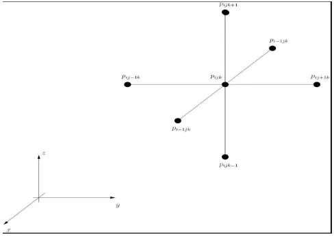
whereAis a matrix which reflects the coefficients in Equation 4.1. The vector variablexrepresents the unknown pressures (one unknown per grid cell) andb is a constant which is computed based on the pressures calculated at the previous time step. Equation 4.2 provides the solution to a pressure per grid cell. Figure 4.1 shows a numerical stencil for a 3-D block:
xijk=pijk i= 1. . . , Nx, j= 1, . . . , Ny, k= 1, . . . , Nz (4.2)
whereNxis the number of cells of the oil reservoir in thexdirection,Ny is the number of cells of the reservoir
in theydirection andNz is the number of cells of the reservoir in thez direction. From a programming model
point of view, and for the rest of the paper we will useA, x, and bas notations to represent the linear system of equations generated in a time step.
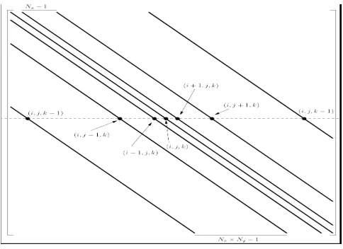
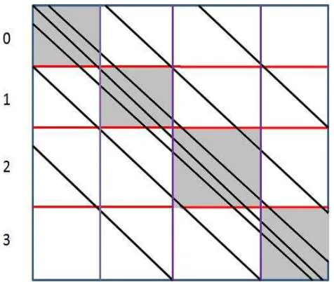
Figure 4.2 shows a computational mesh for a discretized 3-D oil reservoir of size N (N = NxNyNz),
which is the size of the generated matrix A. The mesh reveals the way the unknown vector is composed. By numbering the unknowns, the resulting linear system of equations following a discretization is represented by a heptadiagonal structured sparse matrix as shown in Figure 4.3.
Fig. 4.1: A numerical stencil for a 3-D oil reservoir block.
5. Programming Model.
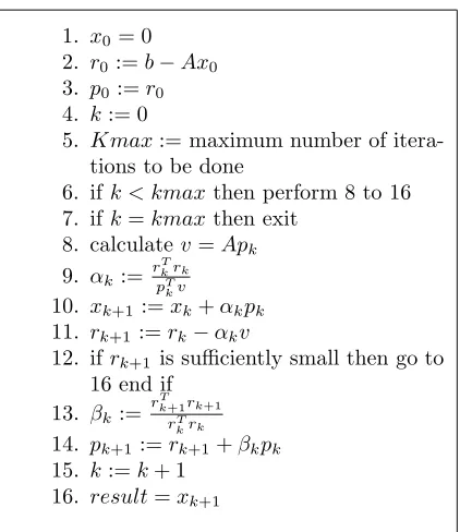
5.1. Sequential CG Algorithm. As shown in Figure 5.1, the CG method starts with a random initial guess of the solutionx0 (step 1). Then, it proceeds by generating vector sequences of iterates (i.e., successive
Fig. 4.2: Computational mesh for discretized 3-D oil reservoir.
Fig. 4.3: Heptadiagonal coefficient matrix formed from a discretized 3-D oil reservoir.
5.2. Parallel Computation Approach. An oil reservoir simulator along with its CG method solver can be parallelized in different ways. Time parallelism, data parallelism and functional parallelism are common approaches for parallelizing applications. In this work, we choose a mix of functional and data parallelism to parallelize the simulator. The simulator is intuitively divided into 2 functional parts: the simulator itself which includes the numerical discretized part and the CG method iterative solver for solving the numerical system of equations. The CG method is used at every time step. Every time step of the oil reservoir simulator produces a linear system of equations.
We chose the master-worker model [28] as an underlying mechanism of parallelization. The simulator itself is executed sequentially by the master processor. The master processor computes various coefficients and parameters and distributes the matrix relative to the resultant linear system of equations to the available processors who will start the parallel processing of finding a solution. The master processor gathers the output from the different processors involved in the computation which forms the global solution. In each iteration of the CG method, each computational component can be parallelized to compute part of the output values: αk,
xk+1, rk+1, βk, andpk+1. To achieve the load balancing the number of non-zero values is distributed equally
over the number of processors in a greedy-based approach.
1. x0= 0
2. r0:=b−Ax0
3. p0:=r0
4. k:= 0
5. Kmax:= maximum number of itera-tions to be done
6. ifk < kmaxthen perform 8 to 16 7. ifk=kmaxthen exit
8. calculate v=Apk
9. αk:= r T krk pT
kv
10. xk+1 :=xk+αkpk
11. rk+1 :=rk−αkv
12. ifrk+1 is sufficiently small then go to
16 end if 13. βk:=
rT k+1rk+1
rT krk
14. pk+1 :=rk+1+βkpk
15. k:=k+ 1 16. result=xk+1
Fig. 5.1: CG method sequential algorithm.
(SpMV) presented in step 8 of the flowchart, and 2) the scalar-vector and/or vector-vector operations presented in steps 9, 10, 11, 13, and 14 of the flowchart. However, CG method presents interdependency between its com-putational elements. In previous work [29], we defined a dependency graph among the different comcom-putational parts of the CG as shown in Figure 5.2. This dependency graph gives directions of data flow within one iteration within a processor and among the processors of the system. The graph shows values which are dependent on other values which are connected to and which are higher in the graph representation. For example, αk is
dependent onrk andpk.
Fig. 5.2: Dependency graph among the different computational elements of the CG method.
For storing the matrix, we use our indexing approach, where the matrix is stored in 2 arrays: a first array which holds the non-zero values and a second array which holds the coordinates of the value in the matrix.
total number of non-zeros in thosen rows are exactly equal to or just more than the calculated average load value. Once the load for a processor in terms of the non-zeros allocated to the processor is calculated, the master processor recalculates the new remaining zeros in the matrix by subtracting the number of non-zeros allocated to the processor from the existing value of the remaining non-non-zeros. Initially all the non-non-zeros in the matrixA are the remaining non-zeros. Then, the master processor calculates a new average load value (in terms of non-zeros) from the number of remaining non-zeros and the number of remaining processors. The master processor allocates the average number of non-zero elements to the next processor and repeats the same steps till all the non-zero values of the matrix A are allocated to the processors. Since we are using greedy approach for the load distribution purpose and the rows are considered as a unit (fraction of the rows are not given to any process), the method is semi-optimized. Appendix A shows the load balancing algorithm.
Given the interdependency nature of the CG method among its computational steps at each each iteration, the SpMV in step 8 should be distributed in a way to decrease communication cost [30]. We rely on a ring-based approach which allows communications and computations to overlap [11] for the SpMV part in each iteration of the CG. The algorithm works as follows. For the entire local SpMV, every processor needs the wholepvector. Every processor divides its local SpMV into N steps, where N is the number of processors involved in the computation. Initially, every processor has its own part of the vectorp. In each step, before starting the local SpMV, a processor sends its own part of the vectorp, in a non-blocking communication, to the left neighbor and simultaneously receive part of the vector p from right neighbor forming a ring of communication. The communication takes place in the form of a ring. Figure 5.3 illustrates the starting computational part in each processor. The local SpMV starts on the block number for which the processor has its own chunk of p. The local SpMV is performed using the non-zero elements of the respective blocks. Figure 5.4 shows an example of the computational steps of the processor of rank 0. Appendix B shows the algorithm of the ring-based approach applied to the matrix-vector multiplication step of the CG method.
Fig. 5.3: Initialization of Computing at every processor.
6. Evaluation of the Parallel Algorithm. In this section, we evaluate the performance of the ring-based parallel oil-phase reservoir simulator in our experimental environment. We compare the performance of our approach to PETSc-based parallel oil reservoir simulator.
Fig. 5.4: The different computational steps for computing the local SpMV in each processor.
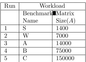
Table 6.1: Experimental Runs
Run Workload
Benchmark Name
Matrix Size(A)
1 S 1400
2 W 7000
3 A 14000
4 B 75000
5 C 150000
6.2. Experiments. The experiments use matrices of different dimensions to assess the performance of the parallel oil reservoir simulator within one step on a single Intel parallel machine and on a grid of Intel parallel machines. The matrix sizes used are as per NAS CG parallel benchmark [26], as shown in Table 6.1. The parallel oil reservoir simulator is measured by horizontally scaling the number of cores up to 128 cores, and vertically scaling the simulation size. The speedup of the parallel parallel oil reservoir versus its sequential execution is measured. We implemented 2 versions of the parallel oil reservoir simulator, one which uses our ring-based approach, and one which uses the PETSc approach in parallelization.
In our experiments, one core acts as a master which distributes the tasks to the other cores that we call workers. The master core runs the simulation, updates and distributes the coefficients; i.e. the matrix, to the workers cores. Thegettimeofday function is used to compute the elapsed time of the parallel oil reservoir simulator on the master in a single time step. In the sequential execution case, thegettimeofday function is used as well to compute the overall run time. In all our experiments, each experiment was run 100 times and the average was computed. The speedup is then measured.
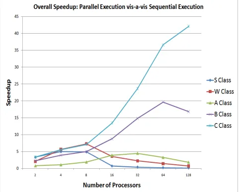
algorithm, which is 42 times faster than the sequential execution of the simulation using 128 processors . It also shows that our parallel implementation scales well with increasing number of processors and large matrix sizes. For instance class C matrix size scales well with increasing number of processors. This is explained by a good overlap between computation and communication for large matrix sizes thanks to a higher number of non-zeros which is allocated to each processor compared to smaller matrix sizes. While our PETSc-based implementation indicates a good speedup of 42.7, as shown in Figure 6.2 for class B matrix size, the speedup performance does not scale with increasing number of processors. The PETSc-based approach has lower scalability compared to our approach with increasing matrix size and increasing number of processors. This is due to the PETSc using asynchronous all-to-all broadcast of the vectorpwhile a local matrix-vector multiplication is taking place. Consequently, the size and the number of vectors exchanged between the processors increase with increasing matrix size and increasing number of processors.
For smaller matrix sizes (classesSandW), our parallelization approach does not scale beyond 8 cores. This is because some processors receive little or no data and therefore the actual computing time can be much shorter than the time spent in communicating the vectorpto other processors; i.e., the processors spend the time waiting for the vectorp to arrive than computing. Therefore, more time is spent in communicating than computing and consequently the overall execution time of the application will become longer in case the computation is divided further over a larger number of processors. The PETSc-based approach has better performance than our approach for small matrix sizes and small number of processors, where the communication time spent communicating the vectorpbetween the processors is overlapped with the local computing on each processor. Implementing a ring-based required more design efforts for the code for communicating the vectorpthan implementing using PETSc approach. Using PETSc, the code calls high level methods and the parallel im-plementation is done by the underlying library, while in a ring-based approach, the dispatch of the vector p to the next neighbor and the reception of the vectorpfrom the previous neighbor have to be done before the matrix-vector multiplication within each processor as shown in Appendix B.
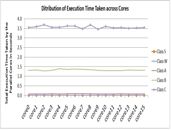
The greedy approach we use for distributing data ensures load balancing as shown in Figure 6.3. However, Figure 6.3 shows slight discrepancies in load among the processors. This is due to the fact that we do not allow for a partial distribution of a matrix row to the processors. Consequently, some processors may be allocated more non-zero values than others.
Fig. 6.1: Overall speedup of a parallel 3-D oil-phase reservoir simulator using our approach vis-a-vis its sequential execution.
Fig. 6.2: Overall speedup of a parallel 3-D oil-phase reservoir simulator using PETSc vis-a-vis its sequential execution.
Fig. 6.3: Distribution of execution time taken across the parallel cores.
then be conducted similar to the one performed for our work published in IEEE Transactions on parallel and distributed systems [32].
8. Acknowledgements. The author would like thank the UAE University for supporting this work, which was funded following a national funding competition organized by the UAE National Research Foundation. She would also like to thank Professor Jamal Abou-Kassem from Petroleum Engineering of the UAE University for his help and availability on many useful discussions on oil reservoir simulator. Special thanks to Professor Eyad Abed, the Dean of the Faculty of Information Technology of the UAE University for his inputs and feedback on the paper. Also, thanks to the anonymous reviewers for their feedbacks which have contributed to the paper.
Appendix A. Load Balancing Algorithm.
loadBalance( ){
//nnz is the number of non-zero values in the matrix
//nnzLeft is the number of non-zeros left out of the cumulative distributions int i=0,j=0,k=0;
//The starting row index of the matrix part and the number of rows to be allocated to a process int *procStartRow, *procCalcRowCount;
//stores number of non zeroes in each row int *rowDataCount;
//The number of non-zeros allocated to a processor int *nnzProc;
//Average load (number of non-zeros) to be distributed to each worker avgLoad = nnz/size;
//Loop over the number of available processors for(i=0; i≤numberOfProcessors-1; i++){
//The beginning row index of the next process is equal to the previous process row index // added to the load allocated to the previous processes
processStartRow[i] = processStartRow[i-1] + procCalcRowCount[i-1] //Compute the actual load to be allocated to the process
for (j=0; j≤N-1, j++){
k = 1;
nnzProc[i]= nnzProc[i]+rowDataCount[k]; k = k+1;
procCalcRowCount[i]=k;
nnzProc[i]= nnzProc[i]+rowDataCount[k]; if (nnzProc[i]≥avgLoad)
break;
}
nnzLeft=nnzLeft-nnzProc[i];
int remainingProcessors = numberOfProcessors-1; avgLoad = nnzLeft/remainingProcessors;
} }
REFERENCES
[1] Abou-Kassem, J.H., Farouq Ali, S.M., and Islam, M.R., 2006, ”Petroleum Reservoir Simulation: A Basic Approach”, Gulf Publishing Company, Houston, TX, USA, 480 pp.
[2] J. Aarnes et al, ”Towards Reservoir Simulation on Geological Grid Models”, 9th European Conference on the Mathematics of Oil Recovery, Cannes, France, September 2004.
[3] Dogru, Ali h., ”From Mega-Cell to Giga-Cell Reservoir Simulation”, Saudi Aramco Journal of Technology, Spring 2008. [4] M.R. Hestenes and E. Stiefel, ”Methods of conjugate gradients for solving linear systems”, J. Research of the National Bureau
Appendix B. Ring-Based Distribution Algorithm.
parallelMultiplyBlocks(double *vecResult, double **AM atrix,double *p, int *nnzLocalBlock){
//List of parameters of the function parllelMultiplyBlocks: // vecResult stores the result of the local SpMV by the processor //AM atrix: Matrix A, stored in a 2D array to represent blocks
//nnzLocalBlocksis the number of local blocks in a local matrix to a processor //neighbourBack,neighbourN extare ranks of neighbours:
// back is the one to send to ahead and next is the one from whom to receive
// pChunkNumber is the id of the processor which uses the current part of P (the chunk from where the MVM will start for a processor
// pChunkNumberNext is the ID for processor from whom to receive chunk of P
int neighbourBack,neighbourNext, pChunkNumber, pChunkNumberNext;
pChunkNumber = processorNumber; // we shall start from blockid = processorNumber.
pChunkNumberNext = (processorNumber + 1) % numberOfProcessors; // we will recveive from next // neighbour
for(int h = 0;h≤numberOfProcessors-1;h++){// h loops over blocks if( h = numberOfProcessors-1 ){
//Asynchronous send of the part of the vectorpthat the processor has updated it to the back neighbor asynchronousSend( &p[pChunkNumber], neighbourBack);
//Asynchronous received of the part of the vectorpfrom the next neighbor asynchronousReceive( &p[pChunkNumber], neighbourNext);
}
//local matrix-vector multiplication on the current block for(int i = 0;i≤nnzLocalBlock[pChunkNumber]-1;i++){
vectorResult=AMatrix*p;
}
//wait to receive the chunk of the vectorpfrom the neighbor if( h = numberOfProcessors -1){
Wait(p);
}
pChunkNumber = pChunkNumberNext;
pChunkNumberNext = (pChunkNumberNext+1) % numberOfProcessors;
} }
[5] Jonathon Richard Shewchuk, ”An Introduction to the Conjugate Gradient Method Without the Agonizing Pain”, School of Computer Science, Carnegie Mellon University, Edition 1 1/4.
[6] Dianne P. O’Leary, ”Parallel Implementation of the Block Conjugate Gradient Algorithm”, Parallel Computing, Vol. 5, pp. 127 - 139, 1987.
[7] Dianne P. O’Leary, ”The Block Conjugate Gradient Algorithm and Related Methods”, Linear Algebra and its Applications, Vol. 29, pp. 293 - 322, 1980.
[8] J. M. Gratien, T. Guignon, J. F. Magras, P. Q. Quandalle, and O. R. Ricois, ”Scalability and Load Balancing Problems in Parallel Oil Reservoir Simulation”, 10th European Conference on the Mathematics of Oil Recovery, September 2006. [9] Cao, H., Tchelepi, H. A., Wallis, J. R., and Yardumian, H., 2005, ”Parallel Scalable Unstructured CPR-Type Linear Solver for
Reservoir Simulation,” paper SPE 96809 presented at the 2005 SPE Annual Technical Conference and Exhibition, Dallas, Texas, USA, Oct. 9 - 12, 2005.
[10] Jesper Larsen, Lars Frellesen, John Jansson, Flemming If, Cliff Addison, Andy Sunderland and Tim Oliver, ”Parallel Oil reservoir Simulation”, Applied Parallel Computing Computations in Physics, Chemistry and Engineering Science Lecture Notes in Computer Science, 1996, Volume 1041/1996, 371-379.
[11] Mark Hoemmen, ”Communication-Avoiding Krylov Subspace Mehthods”, PhD Disseration, Spring 2010, http://www.cs.berkeley.edu/ mhoemmen/pubs/thesis.pdf
[12] Portable, Extensible Toolkit for Scientific Computation, http://www.mcs.anl.gov/petsc/index.html
[13] The Center for Petroleum and Geosystems Engineering, University of Texas at Austin,”Reservoir Simulation Joint Industry Project”, http://www.cpge.utexas.edu/rsjip/
[15] Lois Curfman Mcinnes, and Barry F. Smith, ”PETSC 2.0: A Case Study of using MPI to Develop Numerical Software Libraries”, Proceeding of the Euro-Par’99 parallel processing: 5th International Euro-Par Conference, 1999.
[16] Lu, P., Shaw, J.S., Eccles, T.K., Mishev, I.D., Usadi, A.K., Beckner, B.L., ”Adaptive Parallel Reservoir Simulation,” paper IPTC 12199 presented at the International Petroleum Technology Conference, December 2008.
[17] Khashan, S.A., and Ogbe, D.O., and and Jiang, T.M,, 2002, ”Development and Optimization of Parallel Code for Large-Scale Petroleum Reservoir Simulation,” J. Can. Petrol. Techno., vol. 41, no. 4, 33-37.
[18] Atan, S., Kazemi, H., and Caldwell, D.H., 2006, ”Efficient Parallel Computing Using Multiscale Multimesh Reservoir Simu-lation,” paper SPE 103101presented at the 2006 SPE Annual Technical Conference and Exhibition held in San Antonio, Texas, U.S.A., 24-27 September.
[19] Kevin B. Theobald, Gagan Agrawal, Rishi Kumar, Gerd Heber, Guang R. Gao, Paul Stodghill, and Keshav Pingali, ”Landing CG on EARTH: A Case Study of Fine-Grained Multithreading on an Evolutionary Path”, Proceedings of the ACM/IEEE conference on Supercomputing, pp. 4 - 4, 2000
[20] Fei Chen, Kevin B. Theobald, and Guang R. Gao, ”Implementing Parallel Conjugate Gradient on the EARTH Multithreaded Architecture”, Sixth IEEE International Conference on Cluster Computing, pp. 459 - 469, 2004.
[21] Piero Lanucara, and Sergio Rovida, ”Conjugate Gradients Algorithms: An MPI-OpenMP Implementation on Distributed Shared Memory Systems”, First European Workshop on OpenMP, 1999.
[22] P. Kloos, P. Blaise, and F. Mathey, ”Open MP and MPI Programming with a CG Algorithm”, Proceedings of the European Workshop on OpenMP, 2000.
[23] Marty R. Field, ”Optimizing a Parallel Conjugate Gradient Solver”, SIAM Journal on Scientific Computing, Vol. 19, issue 1, pp. 27 - 37, 1998.
[24] Lewis and Van de Geijn, ”Distributed memory matrix-vector multiplication and conjugate gradient algorithms”’, in Proc. Supercomputing’93, Portland, Oregon, pp. 484-492.
[25] John G. Lewis, David G. Payne, ”Matrix-vector multiplication and conjugate gradient algorithms on distributed memory computers”, in Proc. Scalable High Performance Computing Conference, 1994, pp. 542-550.
[26] D. Bailey, E. Barszcz, J. Barton, D. Browning, R. Carter, L. Dagum, R. Fatoohi, S. Fineberg, P. Frederickson, T. Lasinski, R. Schreiber, H. Simon, V. Venkatakrishnan and S. Weeratunga, ”The NAS Parallel Benchmarks”, RNR Technical Report RNR-94-007, March 1994.
[27] John R. Fanchi, ”Principles of Applied Reservoir Simulation”, ISBN 13: 978-0-7506-7933-6, Elsevier, 2006. [28] Ian Foster, Designing and Building Parallel Programs, Addison- Wesley (ISBN 9780201575941), 1995.
[29] Leila Ismail, ”Communication Issues in Parallel Conjugate Gradient Method using a Star-Based Network”. 2010 International Conference on Computer Applications and Industrial Electronics (ICCAIE 2010),December 2010.
[30] Leila Ismail, k. Shuaib, ”Empirical Study for Communication Cost of Parallel Conjugate Gradient on a Star-Based Network”, ams, pp.498-503, In Proceedings of The 2010 Fourth Asia International Conference on Mathematical/Analytical Modeling and Computer Simulation, 2010, May 2010.
[31] William Gropp, Steven Huss-Lederman, Andrew Lumsdaine, Ewing Lusk, Bill Nitzberg, William Saphir and Marc Snir, ”MPI: The Complete Reference”, Vol. 2, ISBN-10:0-262-57123-4, ISBN-13:978-0-262-57123-4.
[32] Leila Ismail, Driss Guerchi, ”Performance Evaluation of Convolution on the Cell Broadband Engine Processor,” IEEE Trans-actions on Parallel and Distributed Systems, vol. 22, no. 2, pp. 337-351, Feb. 2011, doi:10.1109/TPDS.2010.70.
Edited by: Dana Petcu and Daniela Zaharie
Received: March 1, 2012