M E T H O D O L O G Y
Open Access
Dynamic interaction network inference
from longitudinal microbiome data
Jose Lugo-Martinez
1†, Daniel Ruiz-Perez
2†, Giri Narasimhan
2,3*and Ziv Bar-Joseph
1*Abstract
Background: Several studies have focused on the microbiota living in environmental niches including human body sites. In many of these studies, researchers collect longitudinal data with the goal of understanding not only just the composition of the microbiome but also the interactions between the different taxa. However, analysis of such data is challenging and very few methods have been developed to reconstruct dynamic models from time series microbiome data.
Results: Here, we present a computational pipeline that enables the integration of data across individuals for the reconstruction of such models. Our pipeline starts by aligning the data collected for all individuals. The aligned profiles are then used to learn a dynamic Bayesian network which represents causal relationships between taxa and clinical variables. Testing our methods on three longitudinal microbiome data sets we show that our pipeline improve upon prior methods developed for this task. We also discuss the biological insights provided by the models which include several known and novel interactions. The extended CGBayesNets package is freely available under the MIT
Open Source license agreement. The source code and documentation can be downloaded fromhttps://github.com/
jlugomar/longitudinal_microbiome_analysis_public.
Conclusions: We propose a computational pipeline for analyzing longitudinal microbiome data. Our results provide evidence that microbiome alignments coupled with dynamic Bayesian networks improve predictive performance over previous methods and enhance our ability to infer biological relationships within the microbiome and between taxa and clinical factors.
Keywords: Dynamic interaction network inference, Longitudinal microbiome analysis, Microbial composition prediction, Dynamic Bayesian networks, Temporal alignment
Background
Multiple efforts have attempted to study the microbiota living in environmental niches including human body sites. These microbial communities can play beneficial as well as harmful roles in their hosts and environments. For instance, microbes living in the human gut perform numerous vital functions for homeostasis ranging from harvesting essential nutrients to regulating and maintain-ing the immune system. Alternatively, a compositional imbalance known as dysbiosis can lead to a wide range
*Correspondence:[email protected];[email protected];[email protected]
†Jose Lugo-Martinez and Daniel Ruiz-Perez contributed equally to this work.
1Computational Biology Department, School of Computer Science, Carnegie Mellon University, 5000 Forbes Avenue, Pittsburgh 15213, Pennsylvania, USA 2Bioinformatics Research Group (BioRG), Florida International University, 11200 SW 8th Street, Miami 33199, Florida, USA
Full list of author information is available at the end of the article
of human diseases [1], and is linked to environmental problems such as harmful algal blooms [2].
While many studies profile several different types of microbial taxa, it is not easy in most cases to uncover the complex interactions within the microbiome and between taxa and clinical factors (e.g., gender, age, ethnicity). Microbiomes are inherently dynamic, thus, in order to fully reconstruct these interactions, we need to obtain and analyze longitudinal data [3]. Examples include char-acterizing temporal variation of the gut microbial com-munities from pre-term infants during the first weeks of life, and understanding responses of the vaginal micro-biota to biological events such as menses. Even when such longitudinal data is collected, the ability to extract an accurate set of interactions from the data is still a major challenge.
To address this challenge, we need computational time-series tools that can handle data sets that may exhibit missing or noisy data and non-uniform sampling. Furthermore, a critical issue which naturally arises when dealing with longitudinal biological data is that of tem-poral rate variations. Given longitudinal samples from different individuals (for example, gut microbiome), we cannot expect that the rates in which interactions take place is exactly the same between these individuals. Issues including age, gender, external exposure, etc. may lead to faster or slower rates of change between individuals. Thus, to analyze longitudinal data across individuals, we need to first align the microbial data. Using the aligned profiles, we can next employ other methods to construct a model for the process being studied.
Most current approaches for analyzing longitudinal microbiome data focus on changes in outcomes over time [4, 5]. The main drawback of this approach is that indi-vidual microbiome entities are treated as independent outcomes, hence, potential relationships between these entities are ignored. An alternative approach involves the use of dynamical systems such as the general-ized Lotka-Volterra (gLV) models [6–10]. While gLV and other dynamical systems can help in studying the stability of temporal bacterial communities, they are not well-suited for temporally sparse and non-uniform high-dimensional microbiome time series data (e.g., lim-ited frequency and number of samples), as well as noisy data [3, 10]. Additionally, most of these meth-ods eliminate any taxa whose relative abundance profile exhibits a zero entry (i.e., not present in a measur-able amount at one or more of the measured time points. Finally, probabilistic graphical models (e.g., hidden Markov models, Kalman filters, and dynamic Bayesian networks) are machine learning tools which can effec-tively model dynamic processes, as well as discover causal interactions [11].
In this work, we first adapt statistical spline estimation and dynamic warping techniques for aligning time-series microbial data so that they can be integrated across individuals. We use the aligned data to learn a Dynamic Bayesian Network (DBN), where nodes represent micro-bial taxa, clinical conditions, or demographic factors and edges represent causal relationships between these enti-ties. We evaluate our model by using multiple data sets comprised of the microbiota living in niches in the human body including the gastrointestinal tract, the urogenital tract, and the oral cavity. We show that models for these systems can accurately predict changes in taxa and that they greatly improve upon models constructed by prior methods. Finally, we characterize the biological relation-ships in the reconstructed microbial communities and discuss known and novel interactions discovered by these models.
Methods Data sets
We collected multiple public longitudinal microbiome data sets for testing our method. Additional file1: Table S1 summarizes each longitudinal microbiome data set used in this study, including the complete list of clinical features available.
Infant gut microbiome This data set was collected by La Rosa et al. [5]. They sequenced gut microbiomse from 58 pre-term infants in neonatal intensive care unit (NICU). The data was collected during the first 12 weeks of life (until discharged from NICU or deceased) sampled every day or two on average. Following analysis, 29 micro-bial taxa were reported across the 922 total infant gut microbiome measurements. In addition to the taxa infor-mation, this data set includes clinical and demographic information for example, gestational age at birth, post-conceptional age when sample was obtained, mode of delivery (C-section or vaginal), antibiotic use (percentage of days of life on antibiotic), and more (see Additional file1: Table S1 for complete list of clinical features avail-able).
Vaginal microbiome The vaginal microbiota data set was collected by Gajer et al. [4]. They studied 32 reproductive-age healthy women over a 16-week period. This longitudinal data set is comprised of 937 self-collected vaginal swabs and vaginal smears sampled two times a week. Analysis identified 330 bacterial taxa in the samples. The data also contains clinical and demo-graphic attributes on the non-pregnant women such as Nugent score [12], menses duration, tampon usage, vagi-nal douching, sexual activity, race, and age. To test the alignment methods, we further sub-divided the microbial composition profiles of each subject by menstrual periods. This resulted in 119 time-series samples, an average of 3– 4 menstrual cycles per woman. Additional file2: Figure S1a shows four sub-samples derived from an individual sample over the 16-week period along with corresponding menses information.
samples during gestation from Caucasian women in the control group to reduce potential confounding factors. This restricted set contains 374 temporal samples from 18 pregnant women.
Temporal alignment
As mentioned in the “Background” section, a challenge when comparing time series obtained from different indi-viduals is the fact that while the overall process studied in these individuals may be similar, theratesof change may differ based on several factors (age, gender, other diseases, etc.). Thus, prior to modeling the relationships between the different taxa we first align the data sets between indi-viduals by warping the time scale of each sample into the scale of another representative sample referred to as the reference. The goal of an alignment algorithm is to determine, for each individuali, a transformation func-tionτi(t) which takes as an input a reference timetand outputs the corresponding time for individual i. Using this function, we can compare corresponding values for all individuals sampled for the equivalent time point. This approach effectively sets the stage for accurate discovery of trends and patterns, hence, further disentangling the dynamic and temporal relationships between entities in the microbiome.
There are several possible options for selecting trans-formation functionτi. Most methods used to date rely on polynomial functions [14,15]. Prior work on the analysis of gene expression data indicated that given the relatively small number of time points for each individual simpler functions tend to outperform more complicated ones [16]. Therefore, we used a first-degree polynomial: τi(t) =
(t−b)
a as the alignment function for tackling the temporal alignment problem, whereaandbare the parameters of the function.
Data pre-processing
Since alignment relies on continuous (polynomial) func-tions while the data is sampled at discrete intervals, the first step is to represent the sample data using contin-uous curves as shown by the transition from Fig. 1a to Fig. 1b. Following prior work [16], we use B-splines for fitting continuous curves to microbial composition time-series data, thus, enabling principled estimation of unob-served time points and interpolation at uniform inter-vals. To avoid overfitting, we removed any sample that had less than nine measured time points. The resulting pre-processed data is comprised of 48 individual sam-ples of the infant gut, 116 sub-samsam-ples of the vaginal microbiota, and 15 pregnant women samples of the oral microbiome. We next estimated a cubic B-spline from the observed abundance profile for all taxa in remaining samples usingsplrepandBSplinefrom the Python func-tionscipy.interpolate. In particular,splrepis used to find
the B-spline representation (i.e., vector of knots, B-spline coefficients, and degree of the spline) of the observed abundance profile for each taxa, whereasBSplineis used to evaluate the value of the smoothing polynomial and its derivatives. Additional file3: Figure S2 shows the original and cubic spline of a representative microbial taxa from a randomly selected individual sample across each data set.
Aligning microbial taxon
To discuss the alignment algorithm, we first assume that a reference sample, to which all other samples would be aligned, is available. In the next section, we discuss how to choose such reference.
Formally, letsjr(t)be the spline curve for microbial taxaj at timet∈[tmin,tmax] in the reference time-series sample
r, wheretminandtmaxdenote the starting and ending time points ofsjr, respectively. Similarly, letsji(t)be the spline for individualiin the set of samples to be warped for taxa
jat timet∈tmin , tmax . Next, analogously to Bar-Joseph et al. [14], the alignment error for microbial taxajbetween
sjrandsjiis defined as
ej(r,i)= β
α
sji(τi(t))−sjr(t)
2
dt
β−α ,
where α = max{tmin,τi−1(tmin)} and β = min
tmax,τi−1
tmax correspond to the starting and ending time points of the alignment interval. Observe that by smoothing the curves, it is possible to estimate the values at any intermediate time point in the alignment inter-val [α,β]. Finally, we define the microbiome alignment error for a microbial taxon of interestSbetween individual samplesrandias follows
EM(r,i)=
j∈S
ej(r,i).
Given a referencerand microbial taxonS, the alignment algorithm task is to find parameters aandb that mini-mizeEMfor each individual sampleiin the data set subject to the constraints:a > 0,α < β and (t(β−α)
max−tmin) ≥ .
a
b
c
d
e
f
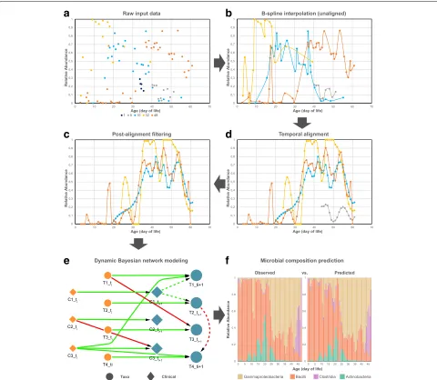
Fig. 1Schematic diagram illustrating the whole computational pipeline proposed in this work. Figure shows microbial taxaGammaproteobacteria
at each step in the pipeline from a set of five representative individual samples (subjects 1, 5, 10, 32, and 48) of the gut data set.aInput is raw relative abundance values for each sample measured at (potentially) non-uniform intervals even within the same subject.bCubic B-spline curve for each individual sample. Sample corresponding to subject 1 (dark blue) contains less than pre-defined threshold for measured time points, thus, removed from further analysis. The remaining smoothed curves enable principled estimation of unobserved time points and interpolation at uniform intervals.cTemporal alignment of each individual sample against a selected reference sample (subject 48 shown in orange).d
Post-alignment filtering of samples with alignment error higher than a pre-defined threshold. Sample corresponding to subject 5 (grey) discarded.e
Learning a dynamic Bayesian network (DBN) structure and parameters. Let nodes (T1,T2,T3,T4) represent microbial taxa and (C1,C2,C3) represent
clinical factors shown as circles and diamonds, respectively. Figure shows two consecutive time slicestiandti+1, where dotted lines connect nodes from the same time slice referred to asintra edges, and solid lines connect nodes between time slices referred to asinter edges. Biological
relationships are inferred from edge parameters in the learned DBN which can be positive (green) or negative (red).fOriginal and predicted relative abundance across four gut taxa for subject 48 at sampling rate of 1 day. Performance is evaluated by average mean absolute error (MAE) between original and predicted abundance values (MAE=0.011)
Selecting a reference sample
Finding an optimal reference that jointly minimizes the error for all samples (EM) is akin to solving a multiple alignment problem. Optimal solutions for such problems still require a runtime that is exponential in the num-ber of samples [14] and so a heuristic approach was used
sample pairs(r,i)without a temporal alignment because overlap constraint is not met. Additionally, we filtered out any microbial taxaj ∈ S for which the mean abundance in eithersjrorsjiwas less than 0.1%, or had zero variance over the originally sampled time points. Lastly, an optimal reference for each data set is determined by generating all possible pairwise alignments between samples. To select the best referencer∗, we employed the following criteria: (1) at least 90% of the individual samples are aligned to
r∗, and (2) the alignment errorEMis minimized. We note that if no candidate reference meets these criteria, a com-monly used heuristic for selectingr∗picks the sample with the longest interval or highest number of measured time points.
Abnormal or noisy samples filtering As a post-processing step, we implemented a simple procedure which takes as input the resulting individual-wise align-ments to identify and filter out abnormal and noisy samples. Given an aligned microbiome data set, we (1) computed the mean μ and standard deviation δ of the alignment errorEMacross all aligned individual samples, and (2) removed all samples from an individual where
EM > μ+(2×δ). Figure1d shows the filtered set for the aligned taxa in the previous step (Fig.1c). This analysis can both help to identify outliers and to improve the ability to accurately reconstruct models for interactions between taxa as shown in “Results” section.
Taxon selection from alignment As previously described, the microbiome alignment error EM for a pairwise alignment is restricted to the set of microbial taxaS that contributed to the alignment. However, this set of microbes can vary for different pairwise alignments even with the same reference. Therefore, we focused on the subset of taxa that contributed to at least half of the pairwise alignments for the selected reference. Additional file4: Table S2 lists alignment information for each data set such as reference sample, number of aligned samples, and selected taxa.
Alignment simulation experiments Since temporal alignment using splines does not guarantee convergence to a global minimum [14], we performed simulation stud-ies to investigate the susceptibility to the non-uniqueness and local optima of the splines-based heuristic approach described at the beginning of this section. In particu-lar, we first used the originally measured time points and observed abundance profile from three taxa of a represen-tative individual sample in the gut data set as the reference sample. We then simulated 10 different individual sam-ples as follows: for each individual sample, we manually warped the time points with randomly selected parame-tersa(scaling) andb(translation) such thata∈(0, 4] and
b∈[ 0, 50]. We next added distinct percentage of Gaussian noise selected from {0, 5, 10, 15, 20, 25} to the warped time points. To further test the robustness of splines, we also added Gaussian noise to the observed abun-dance profile of each taxa. Finally, we conducted three types of simulation experiments: (1) simulated noise-free warped time points for each individual sample but with noisy abundance profile, (2) simulated noise-free abun-dance profile but with noisy warped time points, and (3) noisy simulated warped time points with noisy abundance profiles.
From each simulation experiment, we aligned all simu-lated individual samples to the reference sample. We then computed and reported the mean absolute error (MAE) between the observed alignment parameters (i.e., aand
b), as well as alignment errorEMon the aligned simulated data.
Dynamic Bayesian network models
Bayesian networks(BNs) are a type of probabilistic graph-ical model consisting of a directed acyclic graph. In a BN model, the nodes correspond to random variables, and the directed edges correspond to potential conditional depen-dencies between them. The absence of an edge connect-ing two variables indicates independence or conditional independence between them. Conditional independence allows for a compact, factorized representation of the joint probability distribution [17].
Dynamic Bayesian Networks (DBNs) are BNs better
suited for modeling relationships over temporal data. Instead of building different models across time steps, DBNs allow for a “generic slice” that shows transitions from a previous time point to the next time point, thus representing a generic temporal transition that can occur at any time during the computation. The incorporation of conditional dependence and independence is similar to that in BNs. DBNs have been widely used to model longitudinal data across many scientific domains, includ-ing speech [18, 19], biological [11, 20,21], or economic sequences [22,23].
More formally, a DBN is a directed acyclic graph where, at eachtime slice(or time instance), nodes correspond to random variables of interest (e.g., taxa, post-conceptional age, or Nugent score) and directed edges correspond to their conditional dependencies in the graph. These time slices are not modeled separately. Instead, a DBN con-tains edges connecting time slices known as inter edges
Model construction
Using the aligned time series for the abundance of taxa, we next attempted to learn graphical models that provide information about the dependence of the abundance of taxa on the abundance of other taxa and clinical or demo-graphic variables. Here, we use a “two-stage” DBN model in which only two slices are modeled and learned at a time. Throughout this paper, we will refer to the previ-ous and current time points as ti andti+1, respectively. Fig. 1e illustrates a skeleton of the general structure of a two-stage DBN in the context of a longitudinal micro-biome study. In this example, for each time slice, the nodes correspond to random variables of observed quantities for different microbial taxa (T1,T2,T3,T4) or clinical factors (C1,C2,C3) shown as circles and diamonds, respectively. These variables can be connected by intra edges (dotted lines) or inter edges (solid lines). In this DBN model, the abundance of a particular microbe in the current time slice is determined by parameters from both intra and inter edges, thus, modeling the complex interactions and dynamics between the entities in the microbial community. Typically, analysis using DBNs is divided into two com-ponents: learning the network structure and parameters and inference on the network. The former can be fur-ther sub-divided into (i) structure learning which involves inferring from data the causal connections between nodes (i.e., learning the intra and inter edges) while avoiding overfitting the model, and (ii) parameter learning which involves learning the parameters of each intra and inter edge in a specific network structure. There are only a lim-ited number of open software packages that support both learning and inference with DBNs [24,25] in the presence of discrete and continuous variables. Here, we used the freely available CGBayesNets package [11, 24] for learn-ing the network structure and performlearn-ing inference for Conditional Gaussian Bayesian models [26]. While useful, CGBayesNets does not support several aspects of DBN learning including the use of intra edges, searching for a parent candidate set in the absence of prior information and more. We have thus extended the structure learn-ing capabilities of CGBayesNets to include intra edges while learning network structures and implemented well-known network scoring functions for penalizing mod-els based on the number of parameters such as Akaike Information Criterion (AIC) and Bayesian Information Criterion (BIC) [27].
Learning DBN model parameters Letdenote the set of parameters for the DBN andGdenote a specific net-work structure over discrete and continuous variables in the microbiome study. In a similar manner to McGeachie et al. [11], we can decompose the joint distribution as
P()F( |)=
x∈
p
x|PaG(x)
y∈ f
y|PaG(y)
wherePdenotes a set of conditional probability distribu-tions over discrete variables,F denotes a set of linear Gaussian conditional densities over continuous variables , andPaG(X)denotes the set of parents for variableXin
G. Since we are dealing with both continuous and discrete nodes in the DBN, in our method, continuous variables (i.e., microbial taxa compositions) are modeled using a Gaussian with the mean set based on a regression model over the set of continuous parents as follows
f(y|u1,· · ·,uk)∼N
⎛
⎝λ0+k
i=1
λi×ui,σ2
⎞ ⎠
where u1,· · ·,uk are continuous parents of y; λ0 is the intercept; λ1,· · ·,λk are the corresponding regression coefficients for u1,· · ·,uk; andσ2 is the standard devi-ation. We point out that if y has discrete parents then we need to compute coefficientsL = {λi}ki=0 and stan-dard deviation σ2 for each discrete parents configura-tion. For example, the conditional linear Gaussian den-sity function for variable T4_ti+1 in Fig. 1e denoted as
fT4_ti+1|T4_ti,C3_ti,T2_ti+1 is modeled by
Nλ0+λ1×T4_ti+λ2×C3_ti+λ3×T2_ti+1,σ
2 ,
whereλ1,λ2,λ3, andσ2are the DBN model parameters. In general, given a longitudinal data set D and known structure G, we can directly infer the parameters by maximizing the likelihood of the data given our regression model.
Learning DBN structure Learning the DBN structure can be expressed as finding the optimal structure and parameters
max
,GP(D|,G)P(,G)=P(D,|G)P(G),
where P(D|,G)is the likelihood of the data given the model. Intuitively, the likelihood increases as the number of valid parents PaG(·) increases, thus, making it chal-lenging to infer the most accurate model for data setD. Therefore, the goal is to effectively search over possible structures while using a function that penalizes overly complicated structures and protects from overfitting.
Here, we maximize P(D,|G) for a given structure
not available or difficult to obtain. Next, in order to maxi-mize the full log-likelihood term we implemented a greedy hill-climbing algorithm. We initialize the structure by first connecting each taxa node at the previous time point (for example,T1_tiin Fig.1e) to the corresponding taxa node at
the next time point (T1_ti+1 in Fig.1e). We call this setting
thebaselinemodel since it ignores dependencies between taxa’s and only tries to infer taxa levels based on its lev-els in the previous time points. Next, we added nodes as parents of a specific node via intra or inter edges depend-ing on which valid edge (i.e., no cycles) leads to the largest increase of the log-likelihood function beyond the global penalty incurred by adding the parameters as measured by the BIC1score approximation
BIC(G,D)=logP(D|,G)−d
2logN,
whered= ||is the number of DBN model parameters in
G, andNis the number of time points inD. Additionally, we imposed an upper bound limit on the maximum num-ber of possible parents (maxParents ∈ {1, 3, 5}) for each bacterial nodeX(i.e.,|PaG(X)| ≤maxParents).
Inferring biological relationships
Microbial ecosystems are complex, often displaying a stunning diversity and a wide variety of relationships between community members. These biological relation-ships can be broadly divided into two categories:beneficial
(including mutualism, commensalism, and obligate) or
harmful (including competition, amensalism, and para-sitism). Although the longitudinal data sets considered in this study do not provide enough information to further sub-categorize each biological relationship (e.g., mutual-ism vs. commensalmutual-ism), we use the learned DBN model from each microbiome data set and inspect each interac-tion as a means for inferring simple to increasingly com-plex relationships. For example, consider variableT4_ti in
Fig.1e. Given thattiandti+1represent the previous time point and the current time point (respectively), the pos-sible inference in this case is as follows: edges fromT4_ti
andC3_ti (inter edges) and fromT2_ti+1 (intra edge)
sug-gest the existence of a temporal relationship in which the abundance of taxaT4at a previous time instant and abun-dance of taxaT2 at the current time instant, as well as conditionC3from the previous time instant impact the abundance ofT4at the current time. We previously stated that f(T4_ti+1|T4_ti,C3_ti,T2_ti+1) is modeled byN(λ0+
λ1 × T4_ti + λ2 × C3_ti + λ3 × T2_ti+1,σ2). Therefore,
inspecting the regression coefficients λ1,λ2,λ3 immedi-ately suggests whether the impact is positive or negative. In this example, the regression coefficientsλ1,λ2are pos-itive (λ1,λ2>0) while coefficientλ3is negative (λ3<0), thus, variables T4_ti and C3_ti exhibit positive
relation-ships with microbial taxaT4_ti+1shown as green edges in
Fig.1e, whereas taxaT2_ti exhibits a negative interaction
with T4_ti+1 shown as a red edge (Fig. 1e). This simple
analytic approach enables us to annotate each biological relationship with directional information.
Network visualization
All the bootstrap networks2 shown are visualized using
Cytoscape[31] version 3.6.0, using Attribute Circle Layout with Organic Edge Router. An in-house script is used to generate a custom style XML file for each network, encod-ing multiple properties of the underlyencod-ing graph. Among these properties, the regression coefficients correspond-ing to edge thickness were normalized as follows: let y
be a microbial taxa node with continuous taxa parents
u1,· · ·,ukmodeled by
f(y|u1,· · ·,uk)∼N
⎛
⎝λ0+k
i=1
λi×ui,σ2
⎞ ⎠
whereλ1,· · ·,λk are the corresponding regression coef-ficients for u1,· · ·,uk as previously described in this section. The normalized regression coefficients λNi ki=1 are defined as
λN i =
λi× ¯ui
k
j=1λj× ¯uj ,
where u¯i is the mean abundance of taxa ui across all samples.
Results
Figure 1 presents a schematic diagram illustrating the whole computational pipeline we developed for aligning and learning DBNs for microbiome and clinical data. We start by estimating a cubic spline from the observed abun-dance profile of each taxa (Fig.1b). Next, we determine an alignment which allows us to directly compare temporal data across individuals (Fig.1c), as well as filter out abnor-mal and noisy samples (Fig.1d). Finally, we use the aligned data to learn causal dynamic models that provide infor-mation about interactions between taxa, their impact, and the impact of clinical variables on taxa levels over time (Fig.1e–f ).
Temporal alignments
Below, we discuss in detail the improved accuracy of the learned dynamic models due to use of temporal alignments. However, even before using them for our models, we wanted to verify our splines-based heuristic alignment approach, as well as test whether the alignment results agree with biological knowledge.
Simulation experiments To investigate whether our splines-based greedy alignment approach is able to identify good solutions, we performed several simula-tion experiments (described in “Methods” secsimula-tion). In summary, we simulated data for 10 individual samples and aligned them against a reference sample. We next computed the alignment accuracy (MAE) between the observed and expected alignment parameters (i.e.,aand
b), and alignment errorEMon the simulated data. These results are shown in Additional file5: Figure S3, where the average error for alignment parameteraranges between 0.030 − 0.035 at 5% noise up to 0.24 − 0.35 at 25% noise across all simulation experiments. Alternatively, the average error for alignment parameterbranges between 0.25−0.30 at 5% noise up to 4.5−6.2 at 25% noise across all three experiments. Finally, the alignment error EM is at most 7% at 25% noise which indicates large agreement between the aligned samples. Overall, these simulation results provide evidence that the proposed greedy search method is able to find good alignments, thus, supporting our prior assumptions as well as the use of B-splines.
Infant gut alignments capture gestational age at birth To test whether the alignment results agree with bio-logical knowledge, we used the infant gut data. Infant gut microbiota goes through a patterned shift in dom-inance between three bacterial populations (Bacilli to
GammaproteobacteriatoClostridia) in the weeks imme-diately following birth. La Rosa et al. [5] reported that the rate of change is dependent on maturation of the infant highlighting the importance of post-conceptional age as opposed to day of life when analyzing bac-terial composition dynamics in pre-term infants. We found that our alignment method is able to capture this rate of change without explicitly using gestational or post-conceptional age.
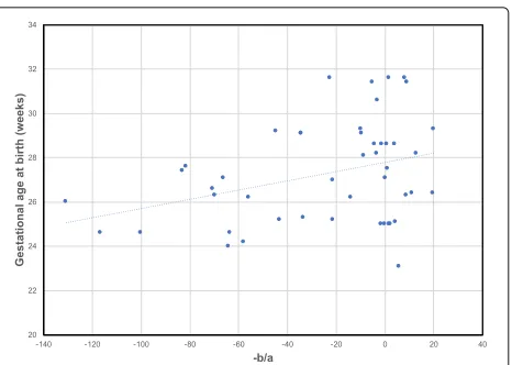
Figure 2 shows the relationship between alignment parameters a and b (from the transformation function τi(t)= (t−ab)described in “Methods” section) and the ges-tational age at birth for each infant in the gut microbiome data set. Each aligned infant sample is represented by a blue circle where thex-axis shows −ab andy-axis shows the gestational age at birth. As can be seen, the alignment parameters are reasonably well correlated with gestational age at birth (Pearson’s correlation coefficient = 0.35)
Fig. 2Relationship between alignment parameters and gestational
age at birth. Figure shows the relationship between alignment parametersaandband gestational age at birth (measured in weeks) for the aligned infant gut microbiome data set. Each blue dot represent an aligned infant sampleiwherex-axis shows−b
a from transformation functionτi(t)= (t−ab)andy-axis shows the gestational age at birth of infanti. Pearson correlation coefficient = 0.35
indicating that this method can indeed be used to infer differences in rates between individuals.
Resulting dynamic Bayesian network models
We next applied the full pipeline to learn DBNs from the three microbiome data sets under study. In particular, we use longitudinal data sets from three human microbiome niches: infant gut, vaginal, and oral cavity as described in “Methods” section. In this section, we highlight the over-all characteristics of the learned DBN for each aligned and filtered microbiome data set (Fig.3and Additional file6: Figure S4a). By contrast, we also show the learned DBN for each unaligned and filtered microbiome data set in Addi-tional file6: Figure S4b and Additional file7: Figure S5. In all these figures, the nodes represent taxa and clinical (or demographic) variables and the directed edges represent temporal relationships between them. Several triangles were also observed in the networks. In some of the trian-gles, directed edges to a given node were linked from both time slices of another variable. We will refer to these as
directed triangles.
a
b
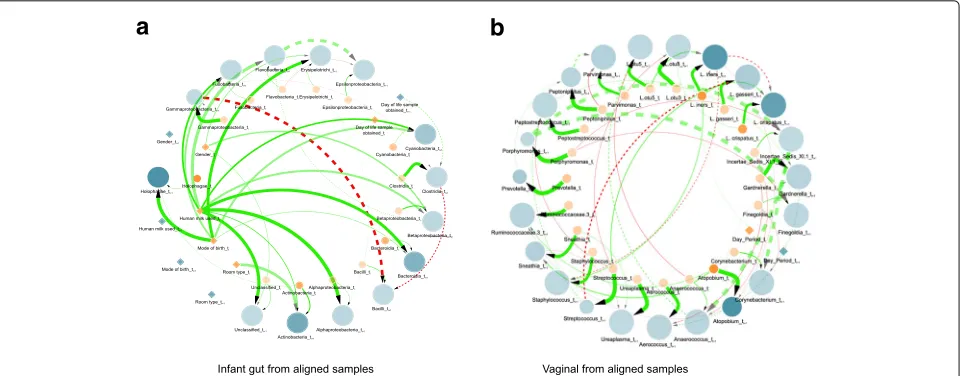
Fig. 3Learned dynamic Bayesian network for infant gut and vaginal microbiomes derived from aligned samples. Figure shows two consecutive
time slicesti(orange) andti+1(blue), where nodes are either microbial taxa (circles) or clinical/demographic factors (diamonds). Nodes size is proportional to in-degree whereas taxa nodes transparency indicates mean abundance. Additionally, dotted lines denoteintra edges(i.e., directed links between nodes in same time slice) whereas solid lines denoteinter edges(i.e., directed links between nodes in different time slices). Edge color indicates positive (green) or negative (red) temporal influence and edge transparency indicates strength of bootstrap support. Edge thickness indicates statistical influence of regression coefficient as described in network visualization.aLearned DBN for the aligned infant gut microbiome data at a sampling rate of 3 days and maxParents = 3.bLearned DBN for the aligned vaginal microbiome data at a sampling rate of 3 days and maxParents = 3
out of 14) have reached the maximum number of parents allowed (i.e.,maxParents = 3). Additionally, the major-ity of these temporal relationships are between microbial taxa. In particular, the model includes several interactions between the key colonizers of the premature infant gut:
Bacilli, Clostridia, and Gammaproteobacteria. Further-more, the only negative interactions learned by the model comprise these microbes which are directly involved in the progression of the infant gut microbiota. Also, the nodes for gestational age at birth and post-conceptional age at birth are not shown because they are isolated from the rest of the network, without any single edge. Overall, these trends strongly suggest that the DBN is capturing biologically relevant interactions between taxa.
Vaginal As with the gut microbiome data set, we learned a DBN model for the vaginal microbiome data at a sampling rate of 3 days and maxParents = 3 (Fig.3b). The resulting DBN is comprised of 24 nodes per time instance (23 taxa and 1 clinical) and 58 edges (40 inter edges and 18 intra edges). Additionally, 12 directed triangles involving taxa nodes were observed. In pre-liminary analyses, additional clinical and demographic attributes (e.g., Nugent category, race, and age group) resulted in networks with these variables connected to all taxa nodes, thus, removed from further analysis. Specif-ically, we estimated the degree of overfitting of these variables by learning and testing DBN models with and without them. This resulted in the DBN shown in Fig.3b which exhibited lowest generalization error. In this case,
the maximum number of potential edges between bacte-rial nodes is 24×maxParents = 72; however, only 16 out of 24 taxa nodes reached the threshold on the maximum number of parents. Among all the 58 edges, only 1 inter-actionDay_Period_ti+1toL. iners_ti+1involves a clinical node whereas the remaining 57 edges (including 15 nega-tive interactions) captured temporal relationships among microbial taxa. This mixture of positive and negative interactions between taxa provides evidence of the DBNs ability to capture the complex relationships and temporal dynamics of the vaginal microbiota.
Oral cavity We learned a DBN with the longitudinal tooth/gum microbiome data set with a sampling rate of 7 days and maxParents = 3. Additional file6: Figure S4a shows the learned DBN which contains 20 nodes for each time slice (19 taxa and 1 clinical) and 52 edges (33 inter edges and 19 intra edges) out of 57 possible edges. In addition, 2 directed triangles were observed involv-ing taxa nodes. Here, the DBN model includes multiple positive and negative interactions among early colonizers (e.g.,VeillonellaandH. parainfluenzae) and late coloniz-ers (e.g.,Porphyromonas) of the oral microbiota which are supported by previous experimental studies [32].
Comparisons to prior methods
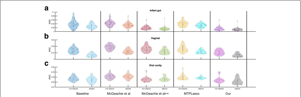
in the literature [11, 33], we used a per-subject cross-validation with the goal of predicting microbial taxon abundances using the learned models. In each iteration, the longitudinal microbial abundance profile of a single subject was selected as the test set, and the remaining profiles were used for building the network and learning model parameters. Next, starting from the second time point, we used the learned model to predict an abundance value for every taxa in the test set at each time point using the previous and current time points. Predicted values were normalized to represent relative abundance of each taxa across the microbial community of interest. Finally, we measured the average predictive accuracy by comput-ing the MAE for the selected taxon in the network. We repeated this process (learning the models and predict-ing based on them) for several different samplpredict-ing rates, which ranged from 1 up to 28 days depending on the data set. The original and predicted microbial abundance pro-files can be compared as shown in Fig. 1f. The average MAE for predictions on the three data sets are summa-rized in Additional file 8: Table S3. Furthermore, Fig. 4 and Additional file9: Figure S6 show violin and bar plots of the MAE distributions for ten different methods on each data set, respectively. Along with two of our DBNs (one with and one without alignments), four methods with and four without alignments were compared. These are further described below.
First, we compared the DBN strategy to a naive (base-line) approach. This baseline approach makes the trivial prediction that the abundance value for each taxa A at any given point is exactly equal to the abundance mea-sured at the previous time point. Given that meamea-sured abundances are continuous variables, this turns out to be an extremely competitive method and performs bet-ter than most prior methods for the data sets we tested
on. Next, we compared our DBNs to three other meth-ods suggested for modeling interactions among taxa: (a) McGeachie et al. [11] developed a different DBN model where network learning is estimated from the BDeu scor-ing metric [24] (instead of MLE), (b) McGeachie et al.++ an in-house implementation that extends McGeachie et al.’s method to allow for intra edges during structure learning, and (c) MTPLasso [33] that models time-series microbial data using a gLV model. In all cases, we used the default parameters as provided in the original publications.
As can be seen by Table S3 and Figure S6, our method outperforms the baseline and previous methods for the infant gut data. It also performs favorably when com-pared to baseline on the other two data sets. Temporal alignments improved the predictive performance over unaligned samples across gut and vaginal microbiomes by about 1–4 percentage points. In particular, a two-tailed t test indicates significant (denoted by *) perfor-mance improvements for most sampling rates (infant gut:
pvalue = 0.043* for 1 day,pvalue = 0.034* for 3 days,
pvalue = 0.109 for 5 days, andpvalue < 1.00E-05* for 7 days; vaginal: p value < 1.00E-06* for 1 day,
pvalue < 1.00E-05* for 3 days,pvalue = 5.50E-05* for 5 days,pvalue = 3.10E-03* for 7 days, andpvalue
= 0.097 for 14 days). On the other hand, alignments did not show significant predictive performance improve-ments on the oral data set and is consistent with previous analysis on the same data set [13]. Surprisingly, the simple baseline approach outperforms all previously published methods: McGeachie et al. [11] and MTPLasso [33] across the three data sets. Finally, Fig. 4 shows violin plots of the MAE results for each data set across a sampling rate that most closely resembles the originally measured time points.
a
b
c
Fig. 4Comparison of average predictive accuracy between methods on the filtered data sets. Figure shows violin plots of the MAE distributions of
Anomaly detection using alignment
When analyzing large cohorts of microbiome data, it is important to implement a strategy to remove outliers as these can affect our ability to generalize from the collected data. As discussed in “Methods” section, we can use our alignment errorEM score to identify such subjects and remove them prior to modeling. In the context of the gut data set, this resulted in the identification of two infant samples: subjects 5 and 55 (highlighted in red within Additional file10: Figure S7a) which are likely processing errors, contaminated samples, or just natural anomalies. Sample 55 has been previously identified as a likely abrup-tion event by McGeachie et al. [11] using a different approach. Similarly, Additional file10: Figure S7b shows the distribution of alignment errors EM for the vaginal microbiome data. In this case, we remove 6 sub-samples from 4 different women (highlighted in red). We note that there were no outliers identified in the oral cavity microbiome data set. When learning DBNs following the filtering we obtain even better models. Additional file11: Figure S8 compares the average MAE results of our pro-posed DBN model between the unfiltered and filtered samples for the gut and vaginal data sets. As can be seen, a large performance improvement is observed for the gut data while a slight improvement is observed for the vagi-nal data when removing the outliers. These results suggest that even though the method uses less data to learn the models, the models that it does learn are more accurate.
Discussion
The power of temporal alignments
We developed a pipeline for the analysis of longitudi-nal microbiome data and applied it to three data sets profiling different human body parts. To evaluate the reconstructed networks we used them to predict changes in taxa abundance over time. Interestingly, ours is the first method to improve upon a naive baseline (Additional file 9: Figure S6). While this does not fully validate the accuracy of the models, it does mean that the additional interactions determined by our method contribute to the ability to infer future changes and so at least some are likely true.
As part of our pipeline, we perform temporal align-ment. While ground truth for alignments is usually hard to determine, in one of the data sets we analyzed we could compare the alignment results to external information to test its usefulness. In the context of the infant gut data, it has been shown that using day of life as the independent variable hinders the identification of associations between bacterial composition and day of sampling. Therefore, previous work have re-analyzed the premature gut micro-biota with post-conceptional age, uncovering biologically relevant relationships [5]. By using alignment we were able to correct for this difference without the need to rely on
the external age information. In addition to the results presented in Fig.2, the learned DBN in Fig.3a does not show any relationships to post-conceptional age or gesta-tional age at birth indicating that our alignment was able to successfully compensate for. By contrast, the learned DBN from unaligned samples in Additional file7: Figure S5a shows relationships to post-conceptional age. While for this data such correction could have been made using post-conceptional age, in other cases the reason for the rate change may not be obvious and without alignment it would be hard to account for such hidden effects.
Uncovering biological relationships
We next discuss in more detail the learned DBN models.
Infant gut As mentioned in “Results” section, the only negative relationships identified supports the known col-onization order, that is, a shift in dominance fromBacilli
toGammaproteobacteriatoClostridia) [5], as the infant goes through the first several weeks of life. These edges show incoming negative relationships to Bacilli from
Gammaproteobacteria and Clostridia. In particular, an increase in the abundance of the parents is associated with a decrease in the abundance of the child. The negative edge from Gammaproteobacteriato Clostridia
agrees with previous findings where Clostridia’s abun-dance is found to increase at a gradual rate until it peaks at post-conceptional age between 33 and 36 weeks whereas Gammaproteobacteriadecreases as infants age [5, 11]. It is important to note that this negative edge from Gammaproteobacteria to Clostridia is not found in the learned DBN from unaligned samples (Additional file7: Figure S5a). This relationship is also confirmed by the edges fromDay of lifetoGammaproteobacteriaand
Clostridia(Fig.3b). Moreover, the DBN model indicates a relationship between breastfeeding andActinobacteria,
Bacteroidia, andAlphaproteobacteria. These bacteria are known to be present in breast milk which is known to heavily influence and shape the infant gut microbiome [34].
Vaginal It has been established that microbial compo-sition can change dramatically during the menses cycle and later return to a ‘stable’ state before the next men-strual period [35,36]. Previous studies have identified a subset of individuals in this data set as exhibiting a micro-bial composition dominated byL. crispatuswith a notable increase of L. iners around the start of each menstrual period [4,35] (Additional file2: Figure S1a). These inter-actions were also captured by the learned DBN model in the form of a directed triangle involvingL. crispatusand
from another group were characterized as dominated by
L. gassericoupled with shifts toStreptococcusduring men-struation [4]. These relationships were also captured by the DBN. Furthermore, whileL. inershas a lower protec-tive value than the otherLactobacillus[37], the negative edge betweenL. inersandAtopobiumsuggests a relation-ship related to environment protection. Also, the positive edge fromAtopobiumtoGardnerellais supported by the synergy observed between these two taxa in bacterial vagi-nosis [38]. Although many of these microbial relationships are also observed in the learned DBN from unaligned sub-samples, there are some biological relationships which cannot be found within the DBN derived without align-ments. However, given our limited understanding of the interactions within the vaginal microbiome, we cannot determine whether or not these previously unseen inter-actions are biologically relevant. Finally, it is worth high-lighting that the shifts and composition of the vaginal microbiome vary considerably between each women [4,36].
Oral For oral microbiomes, severalStreptococcusspecies, includingS. oralis,S. mitis,S. gordonii, andS. sanguisare well known as early colonizers lying close to the tooth pellicle [32]. While our learned DBNs (Additional file6: Figure S4) cannot identify specific species, it suggests interactions between some species of Streptococcusand other later colonizers in the oral microbiome such as Por-phyromonas and Prevotella. The learned DBN derived from aligned tooth/gum samples also provided novel pre-dictions, for example, taxa Granulicatella is interacting with Veilonella. Furthermore, there are other microbial relationships uniquely observed on each DBN which are also potentially interesting.
Triangles in DBNs
An interesting aspect shared by all of the DBNs dis-cussed above is the fact that they contain triangles or feed-forward loops. In particular, many of these directed triangles are created from nodes representing both time slices of another variable, but with different signs (one positive and the other negative). For example, microbial taxaL. crispatusdisplays a directed triangle with another taxaL. inersin the vaginal DBN (Fig.3b). In this triangle, positive edges fromL. iners_ti interact withL. iners_ti+1 andL. crispatus_ti+1whereas a negative edge connectsL.
iners_ti+1toL. crispatus_ti+1.
The triangles in the DBNs represent a relationship where the abundance of a child node cannot be solely determined from the abundance of a parent at one time slice. Instead, information from both the previous and the current time slices is needed. This can be interpreted as implying that the child node is associated with thechange
of the abundance values of the parents rather than with the absolute values which each node represents.
Limitation and future work
While our pipeline of alignment followed by DBN learn-ing successfully reconstructed models for the data sets we looked at, it is important to understand the limi-tation of the approach. First, given the complexity of aligning a large number of individuals, our alignment method is based on a greedy algorithm, thus, it is not guaranteed to obtain the optimal result. Even if the alignment procedure is successful, the DBN may not be able to reflect the correct interactions between taxa. Issues related to sampling rates can impact the accu-racy of the DBN (missing important intermediate inter-actions) while on the other hand if not enough data is available the model can overfit and predict non-existent interactions.
Given these limitations, we would attempt to improve the alignment method and its guarantees in future work. We are also interested in studying the abil-ity of our procedure to integrate additional molecular longitudinal information including gene expression and metabolomics data which some studies are now col-lecting in addition to the taxa abundance data [39]. We believe that our approach for integrating informa-tion across individual in order to learn dynamic mod-els would be useful for several ongoing and future studies.
Conclusions
In this paper, we propose a novel approach to the anal-ysis of longitudinal microbiome data sets using dynamic Bayesian networks with the goal of eliciting temporal rela-tionships between various taxonomic entities and other clinical factors describing the microbiome. The novelty of our approach lies in the use of temporal alignments to normalize the differences in pace of biological processes inherent within different subjects. Additionally, the align-ment algorithm can be used to filter out abruption events or noisy samples. Our results show that microbiome alignments improve predictive performance over previ-ous methods and enhance our ability to infer known and potentially novel biological and environmental relation-ships between the various entities of a microbiome and the other clinical and demographic factors that describe the microbiome.
Endnotes
1We also computed AIC score (i.e., AIC(G,D) = logP(D|,G)−d) but it was consistently outperformed by BIC score.
2For each data set, we ran 500 bootstrap realizations
Additional files
Additional file 1:Table S1.Summary of longitudinal microbiome data sets. For each data set, we show the total number of individualsni, number of time series samplesns, number of microbial taxa reportednt, original sampling rate, and list of clinical attributes available. (PDF 57 kb) Additional file 2:Figure S1.Representative vaginal microbiome sample for subject 28 over the 16-week period.aRelative abundance profile of six vaginal taxa for subject 48 over 16 weeks annotated with menses information. The vertical black lines correspond to the division of sub-samples based on menstrual periods (i.e., 4 sub-samples). Note the interpolated shift in dominance during menses betweenL. crispatusandL. iners.b| Temporal alignment between the sub-samples from subject 28 time-series data for taxaL. crispatususing the first menstrual period sub-sample as reference (shown in orange). Figure also shows abundance profile ofL. crispatusfor each sub-sample before (left) and after (right) alignment. (PDF 431 kb)
Additional file 3:Figure S2.Original and cubic spline of the abundance profile of a representative microbial taxa for each data set. Figure shows the original abundance values vs. the cubic B-spline curve for a representative taxa profile from a randomly selected individual sample across each data set.aBacillifrom the infant gut microbiome.bL. inersfrom the vaginal microbiome.cPrevotellafrom the oral cavity microbiome. (PDF 39 kb) Additional file 4:Table S2.Summary of alignment information. For each data set, we show reference sample, number of aligned samplesnr, and selected taxa. (PDF 61 kb)
Additional file 5:Figure S3.Temporal alignment accuracy on simulated data. Figure shows MAE alongside standard deviation for alignment parametersaandb, as well as alignment errorEMusing our heuristic alignment approach as a function of percentage of Gaussian noise.a Alignment performance on simulation experiment 1.bAlignment performance on simulation experiment 2.cAlignment performance on simulation experiment 3. (PDF 33 kb)
Additional file 6:Figure S4.Learned dynamic Bayesian network of the oral microbiome derived from unaligned and aligned tooth/gum samples. Figure shows two consecutive time slicesti(orange) andti+1(blue), where
nodes are either microbial taxa (circles) or clinical factors (diamonds). Nodes size is proportional to in-degree whereas taxa nodes transparency indicates mean abundance. Additionally, dotted lines denoteintra edgeswhereas solid lines denoteinter edges. Edges color indicates positive (green) or negative (red) temporal influence, and edge transparency indicates strength of bootstrap value. Edge thickness indicates statistical influence of regression coefficient as described in network visualization.aLearned DBN for the aligned oral microbiome data at a sampling rate of 7 days and maxParents =3.bLearned DBN for the unaligned oral microbiome data at a sampling rate of 7 days and maxParents= 3. (PDF 55 kb)
Additional file 7:Figure S5.Learned dynamic Bayesian network for gut and vaginal microbiomes derived from unaligned samples. Figure shows two consecutive time slicesti(orange) andti+1(blue), where nodes are
either microbial taxa (circles) or clinical/demographic factors (diamonds). Nodes size is proportional to in-degree whereas taxa nodes transparency indicates mean abundance. Additionally, dotted lines denoteintra edges
(i.e., directed links between nodes in same time slice) whereas solid lines denoteinter edges(i.e., directed links between nodes in different time slices). Edge color indicates positive (green) or negative (red) temporal influence, and edge transparency indicates strength of bootstrap support. Edge thickness indicates statistical influence of regression coefficient as described in network visualization.aLearned DBN for the unaligned infant gut microbiome data at a sampling rate of 3 days and maxParents=3.b Learned DBN for the unaligned vaginal microbiome data at a sampling rate of 3 days and maxParents =3. (PDF 56 kb)
Additional file 8:Table S3.Summary of average predictive accuracy and standard deviation between methods on the filtered data sets. For each data set, we list the average MAE and standard deviation (presented as percentage) of our proposed DBN models against a baseline method and previously published approaches across different sampling rates. Additionally, each method is run on the non-aligned and aligned data sets.
The highest predictive accuracy for each sampling rate is shown in boldface. (PDF 60 kb)
Additional file 9:Figure S6.Comparison of average predictive accuracy and standard deviation between methods on the filtered data sets. Figure shows the average MAE and standard deviation of our proposed DBN models against a baseline method and previously published approaches as a function of sampling rates. Additionally, each method is run on the unaligned and aligned data sets.aPerformance results for infant gut microbiome data.bPerformance results for vaginal microbiome data.c Performance results for oral cavity microbiome data. (PDF 51 kb) Additional file 10:Figure S7.Distribution of microbiome alignment errorEMfor infant gut and vaginal data sets.aEMscores for 47 infant gut samples aligned against a common reference gut sample.bEMscores for 112 vaginal microbiome sub-samples aligned against an optimal reference sub-sample. In both panels, the scores highlighted in red represent samples withEMat least two standard deviations away from the mean of the distribution of microbiome alignment errors, thus, identified as outliers and removed. (PDF 21 kb)
Additional file 11:Figure S8.Effect of outliers on average predictive accuracy from aligned data sets. Figure shows the average MAE for our proposed DBN model and baseline method as a function of sampling rates before (labeled asunfiltered) and after (labeled asfiltered) removal of outliers.aPerformance results for infant gut microbiome data.b Performance results for vaginal microbiome data. (PDF 30 kb)
Abbreviations
AIC: Akaike information criterion; BDeu: Bayesian Dirichlet equivalent sample-size uniform; BIC: Bayesian information criterion; DBN: Dynamic Bayesian network; gLV: Generalized Lotka-Volterra; MLE: Maximum likelihood estimation; MAE: Mean absolute error; NICU: Neonatal intensive care unit
Acknowledgements
The authors would like to thank Jun Ding for his assistance in implementing the temporal alignment algorithm.
Funding
This work was partially supported by McDonnell Foundation program on Studying Complex Systems (awarded to ZB-J), National Science Foundation (award number DBI-1356505 to ZB-J), National Institute of Health (award number 1R15AI128714-01 to GN), Department of Defense (contract number W911NF-16-1-0494 to GN), and National Institute of Justice (award number 2017-NE-BX-0001 to GN).
Availability of data and materials
All code and longitudinal microbiome data sets can be downloaded from https://github.com/jlugomar/longitudinal_microbiome_analysis_public. All data sets analyzed in this work are derived from the following published articles [and their supplementary information files]: infant gut [5], vaginal [4], and oral cavity [13].
Authors’ contributions
GN and ZB-J conceived the experiments. JL-M, GN, and ZB-J designed the experiments. JL-M and DR-P performed the experiments. DR-P visualized the dynamic Bayesian networks. JL-M, DR-P, GN, and ZB-J analyzed the data. All authors contributed in writing the manuscript, All authors read and approved the final manuscript.
Ethics approval and consent to participate Not applicable.
Consent for publication Not applicable.
Competing interests
The authors declare that they have no competing interests.
Publisher’s Note
Author details
1Computational Biology Department, School of Computer Science, Carnegie
Mellon University, 5000 Forbes Avenue, Pittsburgh 15213, Pennsylvania, USA.
2Bioinformatics Research Group (BioRG), Florida International University, 11200
SW 8th Street, Miami 33199, Florida, USA.3Biomolecular Sciences Institute,
Florida International University, Miami 33199, Florida, USA.
Received: 15 September 2018 Accepted: 11 March 2019
References
1. Cho I, Blaser MJ. The human microbiome: at the interface of health and disease. Nat Rev Genet. 2012;13:260–70.
2. Anderson D. HABs in a changing world: a perspective on harmful algal blooms, their impacts, and research and management in a dynamic era of climactic and environmental change. Harmful Algae. 2012;10:3–17. 3. Gerber GK. The dynamic microbiome. FEBS Lett. 2014;588(22):4131–139. 4. Gajer P, Brotman RM, Bai G, Sakamoto J, Schütte UME, Zhong X, Koenig SSK,
Fu L, Ma ZS, Zhou X, Abdo Z, Forney LJ, Ravel J. Temporal dynamics of the human vaginal microbiota. Sci Transl Med. 2012;4(132):132–52. 5. La Rosa PS, Warner BB, Zhou Y, Weinstock GM, Sodergren E, Hall-Moore CM,
Stevens HJ, Bennett WE, Shaikh N, Linneman LA, Hoffmann JA, Hamvas A, Deych E, Shands BA, Shannon WD, Tarr PI. Patterned progression of bacterial populations in the premature infant gut. Proc Natl Acad Sci. 2014;111(34):12522–7.
6. Chung M, Krueger J, Pop M. Identification of microbiota dynamics using robust parameter estimation methods. Math Biosci. 2017;294:71–84. 7. Marino S, Baxter NT, Huffnagle GB, Petrosino JF, Schloss PD.
Mathematical modeling of primary succession of murine intestinal microbiota. Proc Natl Acad Sci. 2014;111(1):439–44.
8. Stein RR, Bucci V, Toussaint NC, Buffie CG, Rätsch G, Pamer EG, Sander C, Xavier JB. Ecological modeling from time-series inference: Insight into dynamics and stability of intestinal microbiota. PLoS Comput Biol. 2013;9(12):1–11.
9. Trosvik P, Stenseth NC, Rudi K. Characterizing mixed microbial population dynamics using time-series analysis. ISME J. 2008;2:707–15. 10. Gibson TE, Gerber GK. Robust and scalable models of microbiome
dynamics. In: Proceedings of the 35th International Conference on Machine Learning, PMLR Vol. 80. 2018. p. 1763–1772.
11. McGeachie MJ, Sordillo JE, Gibson T, Weinstock GM, Liu YY, Gold DR, Weiss ST, Litonjua A. Longitudinal prediction of the infant gut microbiome with dynamic bayesian networks. Sci Rep. 201620359. 12. Nugent RP, Krohn MA, Hillier SL. Reliability of diagnosing bacterial
vaginosis is improved by a standardized method of gram stain interpretation. J Clin Microbiol. 1991;29(2):297–301. 13. DiGiulio DB, Callahan BJ, McMurdie PJ, Costello EK, Lyell DJ,
Robaczewska A, Sun CL, Goltsman DSA, Wong RJ, Shaw G, Stevenson DK, Holmes SP, Relman DA. Temporal and spatial variation of the human microbiota during pregnancy. Proc Natl Acad Sci. 2015;112(35):11060–5. 14. Bar-Joseph Z, Gerber GK, Gifford DK, Jaakkola TS, Simon I. Continuous
representations of time-series gene expression data. J Comput Biol. 2003;10(3–4):341–56.
15. Smith AA, Vollrath A, Bradfield CA, Craven M. Clustered alignments of gene-expression time series data. Bioinformatics. 2009;25(12):119–27. 16. Bar-Joseph Z, Gitter A, Simon I. Studying and modelling dynamic
biological processes using time-series gene expression data. Nat Rev Genet. 2012;13:552–64.
17. Russell SJ, Norvig P. Artificial intelligence: a modern approach, 2nd edn. Upper Saddle River: Prentice Hall Press; 2003.
18. Nefian AV, Liang L, Pi X, Liu X, Murphy K. Dynamic bayesian networks for audio-visual speech recognition. EURASIP J Adv Signal Proc. 2002;11: 1274–88.
19. Zweig G. Speech recognition with dynamic bayesian networks. PhD thesis. 1998.
20. de Luis Balaguer MA, Fisher AP, Clark NM, Fernandez-Espinosa MG, Möller BK, Weijers D, Lohmann JU, Williams C, Lorenzo O, Sozzani R. Predicting gene regulatory networks by combining spatial and temporal gene expression data in arabidopsis root stem cells. Proc Natl Acad Sci. 2017;114(36):7632–640.
21. Halloran JT, Bilmes JA, Noble WS. Dynamic bayesian network for accurate detection of peptides from tandem mass spectra. J Proteome Res. 2016;15(8):2749–759.
22. Robinson JW, Hartemink AJ. Learning non-stationary dynamic bayesian networks. J Mach Learn Res. 2010;11:3647–680.
23. Weber P, Medina-Oliva G, Simon C, Iung B. Overview on bayesian networks applications for dependability, risk analysis and maintenance areas. Eng Appl Artif Intell. 2012;25(4):671–82.
24. McGeachie MJ, Chang HH, Weiss ST. CGBayesNets: Conditional gaussian bayesian network learning and inference with mixed discrete and continuous data. PLoS Comput Biol. 2014;10(6):1–7.
25. Wilczy `nski B, Dojer N. BNFinder: exact and efficient method for learning bayesian networks. Bioinformatics. 2009;25(2):286–7.
26. Lauritzen SL, Wermuth N. Graphical models for associations between variables, some of which are qualitative and some quantitative. Ann Statist. 1989;17(1):31–57.
27. Penny WD. Comparing dynamic causal models using AIC, BIC and free energy. NeuroImage. 2012;59(1):319–30.
28. Silander T, Kontkanen P, Myllymäki P. On sensitivity of the map bayesian network structure to the equivalent sample size parameter. In: Proc. 23rd Conference on Uncertainty in Artificial Intelligence. UAI ’07. Arlington: AUAI Press; 2007. p. 360–7.
29. Steck H. Learning the bayesian network structure: Dirichlet prior vs data. In: Proc. 24th Conference on Uncertainty in Artificial Intelligence. UAI ’08. Arlington: AUAI Press; 2008. p. 511–8.
30. O’Hagan A, Forster JJ. Kendall’s Advanced Theory of Statistics, Vol. 2B: Bayesian Inference, 2nd edn. London: Edward Arnold Press; 2004. 31. Shannon P, Markiel A, Ozier O, Baliga NS, Wang JT, Ramage D, Amin N,
Schwikowski B, Ideker T. Cytoscape: a software environment for integrated models of biomolecular interaction networks. Genome Res. 2003;13(11):2498–504.
32. Kolenbrander PE, Andersen RN, Blehert DS, Egland PG, Foster JS, Palmer RJ. Communication among oral bacteria. Microbiol Mol Biol Rev. 2002;66(3):486–505.
33. Lo C, Marculescu R. Inferring microbial interactions from metagenomic time-series using prior biological knowledge. In: Proc. 8th ACM Conference on Bioinformatics, Computational Biology, and Health Informatics. ACM-BCB ’17. Arlington: AUAI Press; 2017. p. 168–77. 34. Jost T, Lacroix C, Braegger C, Chassard C. Assessment of bacterial
diversity in breast milk using culture-dependent and
culture-independent approaches. Br J Nutr. 2013;110(7):1253–62. 35. Hickey RJ, Abdo Z, Zhou X, Nemeth K, Hansmann M, Osborn TW,
Wang F, Forney LJ. Effects of tampons and menses on the composition and diversity of vaginal microbial communities over time. BJOG. 2013;120(6):695–706.
36. Ravel J, Gajer P, Abdo Z, Schneider GM, Koenig SSK, McCulle SL, Karlebach S, Gorle R, Russell J, Tacket CO, et al. Vaginal microbiome of reproductive-age women. Proc Natl Acad Sci. 2011;108(Suppl 1): 4680–687.
37. Petrova MI, Reid G, Vaneechoutte M, Lebeer S. Lactobacillus iners: friend or foe? Trends Microbiol. 2017;25(3):182–91.
38. Hardy L, Jespers V, Abdellati S, De Baetselier I, Mwambarangwe L, Musengamana V, van de Wijgert J, Vaneechoutte M, Crucitti T. A fruitful alliance: the synergy between atopobium vaginae and gardnerella vaginalis in bacterial vaginosis-associated biofilm. Sex Transm Infect. 2016;92(7):487–91.