1Ministry of Education Key Laboratory for Earth System Modeling, Center for Earth System Science (CESS), Tsinghua University, Beijing, China
2Department of Computer Science and Technology, Tsinghua University, Beijing, China 3Joint Center for Global Change Studies (JCGCS), Beijing, China
4State Key Laboratory of Numerical Modelling for Atmospheric Sciences and Geophysical Fluid Dynamics (LASG), Institute of Atmospheric Physics, Chinese Academy of Sciences, Beijing, China
Correspondence to:Li Liu ([email protected]) and Guangwen Yang ([email protected]) Received: 22 September 2015 – Published in Geosci. Model Dev. Discuss.: 20 October 2015
Revised: 10 May 2016 – Accepted: 24 May 2016 – Published: 9 June 2016
Abstract.Data transfer means transferring data fields from a sender to a receiver. It is a fundamental and frequently used operation of a coupler. Most versions of state-of-the-art cou-plers currently use an implementation based on the point-to-point (P2P) communication of the message passing inter-face (MPI) (referred to as “P2P implementation” hereafter). In this paper, we reveal the drawbacks of the P2P implemen-tation when the parallel decompositions of the sender and the receiver are different, including low communication band-width due to small message size, variable and high number of MPI messages, as well as network contention. To over-come these drawbacks, we propose a butterfly implemen-tation for data transfer. Although the butterfly implementa-tion outperforms the P2P implementaimplementa-tion in many cases, it degrades the performance when the sender and the receiver have similar parallel decompositions or when the number of processes used for running models is small. To ensure data transfer with optimal performance, we design and implement an adaptive data transfer library that combines the advantages of both butterfly implementation and P2P implementation. As the adaptive data transfer library automatically uses the best implementation for data transfer, it outperforms the P2P implementation in many cases while it does not decrease the performance in any cases. Now, the adaptive data transfer li-brary is open to the public and has been imported into the C-Coupler1 coupler for performance improvement of data transfer. We believe that other couplers can also benefit from this.
1 Introduction
Climate system models (CSMs) and Earth system models (ESMs) are fundamental tools for simulating, predicting, and projecting climate. A CSM or an ESM generally integrates several component models, such as an atmosphere model, a land surface model, an ocean model, and a sea-ice model, into a coupled system to simulate the behaviours of the cli-mate system, including the interactions between components of the climate system. More and more coupled models have sprung up in the world. For example, the number of coupled model configurations in the Coupled Model Intercomparison Project (CMIP) has increased from less than 30 (used for CMIP3) to more than 50 (used for CMIP5).
a Cray XT3 (Dennis, 2007); the Community Atmosphere Model (CAM; Morrison and Gettelman, 2008; Neale et al., 2010, 2012) with a spectral element dynamical core (CAM-SE) at 0.25◦horizontal resolution can scale to 86 000 proces-sor cores on a Cray XT5 (Dennis et al., 2012).
A coupler is an important component in a coupled sys-tem. It links component models together to construct a pled model, and controls the integration of the whole cou-pled model (Valcke et al., 2012). A number of couplers are now available, e.g. the Model Coupling Toolkit (MCT; Ja-cob et al., 2005), the Ocean–Atmosphere–Sea Ice–Soil (OA-SIS) coupler (Redler et al., 2010; Valcke, 2013; Valcke et al., 2015), the Earth system modelling framework (ESMF; Hill et al., 2004), the CPL6 coupler (Craig et al., 2005), the CPL7 coupler (Craig et al., 2012), the flexible modelling system (FMS) coupler (Balaji et al., 2006), the bespoke framework generator (BFG; Ford et al., 2006; Armstrong et al., 2009), and the community coupler version 1 (C-Coupler1; Liu et al., 2014).
A coupler generally has much smaller overhead than the component models in current coupled systems. However, it is potentially a time-consuming component in future coupled models. This is because more and more component mod-els (such as the land-ice model, chemistry model and bio-geochemical model) will be coupled into a coupled model, and the coupling frequency between component models will be higher and higher. Data transfer is a fundamental and frequently used operation in a coupler. It is responsible for transferring data fields between the processes of two compo-nent models and for rearranging data fields among processes of the same component model for parallel data interpolation. A coupler may become a bottleneck for efficient paral-lelization of future coupled models. The most obvious reason is that the current implementation of data transfer in a state-of-the-art coupler may be not efficient enough. For example, due to the low efficiency of data transfer, the coupling from a component model with a horizontal grid (576×384 grid points) to another component model with a different hori-zontal grid (3600×2400 grid points) can only scale to about 500 processor cores when using the CPL7 coupler (Craig et al., 2012). Therefore, it is highly desirable to improve the parallel data transfer of couplers.
In this study, we first propose a butterfly implementation of data transfer. Since the point-to-point (P2P) communication of the message passing interface (MPI) (referred to as “P2P implementation” hereafter) and the butterfly implementation can outperform each other in different cases (Sect. 5), we next develop an adaptive data transfer library that includes both implementations and can adaptively implement the bet-ter one for data transfer. Performance evaluation demon-strates that such a library significantly outperforms the P2P implementations in most cases and does not degrade the per-formance in any case. This library has been imported into the C-Coupler1 with a slight code modification. We believe that other couplers can also benefit from it.
0 0.0005 0.001 0.0015 0.002 0.0025 0.003 0.0035 0.004
6 12 24 48 96 192
T
im
e (
s)
Number of processes per model
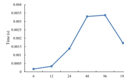
Figure 1.Average execution time of the P2P implementation when transferring 14 2-D fields from CLM3 to GAMIL2. In each test, the atmosphere model GAMIL2 and the land surface model CLM3 have the same number of processes; they do not share the same computing nodes. The horizontal grid of the 14 2-D fields contains 7680 (128×60) grid points.
The remainder of this paper is organized as follows. We briefly introduce the implementation of data transfer in ex-isting couplers in Sect. 2. Details of the butterfly implemen-tation and the adaptive data transfer library are presented in Sects. 3 and 4, respectively. The performances of data trans-fer implementations are evaluated in Sect. 5. Conclusions are given in Sect. 6.
2 Data transfer implementations in existing couplers 2.1 P2P implementation
Almost all state-of-the-art couplers use a similar implemen-tation for data transfer. To achieve parallel data transfer, MCT first generates a communication router (known as the data mapping between processes) according to the parallel decompositions (the distribution of grid points among the processes) of the sender and the receiver, and then uses the P2P communication of the MPI to transfer the data. A data field will be transferred from a process of the sender to a process of the receiver, only when the two processes have common grid points, i.e. “P2P implementation” for short.
Since MCT has already been imported into OASIS3– MCT, the CPL6 coupler, and the CPL7 coupler, these cou-plers also use the P2P implementation for data transfer. Al-though the other couplers, such as ESMF, OASIS4, the FMS coupler, and C-Coupler1, do not directly import MCT, they also use the P2P implementation for data transfer.
2.2 Performance bottlenecks of the P2P implementation
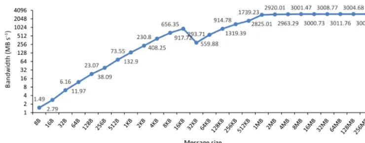
Figure 2.Variation of bandwidth (yaxis) of an MPI P2P communication with respect to the message size (xaxis). The results are generated from our benchmark. In the benchmark, one process sends messages with different sizes to the other process. The two processes of the P2P communication run on two different computing nodes of Tansuo100.
Atmospheric Model of IAP LASG-Version 2)–CLM3 (Com-munity Land Model version 3), which includes GAMIL2 (Li et al., 2013), i.e. an atmosphere model and CLM3 (Oleson et al., 2004; Dickinson et al., 2006), i.e. a land surface model. GAMIL2 and CLM3 share the same horizontal grid of 7680 (128×60) grid points, but have different parallel decompo-sitions: GAMIL2 uses a regular two-dimensional (2-D) allel decomposition, while CLM3 uses an irregular 2-D par-allel decomposition where the grid points are assigned to the processes in a round-robin fashion.
In this benchmark, there is only the data transfer with the P2P implementation between the sender and the receiver with the same horizontal grid as GAMIL2–CLM3. The par-allel decomposition of the sender is derived from CLM3, and the parallel decomposition of the receiver is derived from GAMIL2. A high-performance computer called Tansuo100 at Tsinghua University, China, is used for the performance tests. It has 700 computing nodes, each of which contains two six-core Intel Xeon X5670 CPUs and 32 GB main mem-ory. All computing nodes are connected by a high-speed In-finiBand network with peak communication bandwidth of 5 GB s−1.
To evaluate the parallel performance of the P2P implemen-tation, 14 2-D coupling fields are transferred between the sender and the receiver. In each test, the sender and the re-ceiver use the same number of processes. Since there are 12 processor cores on each computing node, the number of pro-cesses is set to be an integral multiple of 12. The sender and the receiver are located on different computing nodes and the communication of the P2P implementation must go through the InfiniBand network.
Figure 1 demonstrates that the poor parallel scalability of the P2P implementation can be obtained when the parallel decompositions of the sender and receiver are different. It is well known that the communication performance heavily de-pends on message size. As shown in Fig. 2, the P2P commu-nication bandwidth achieved generally increases with
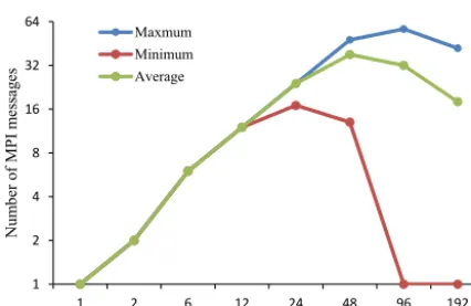
mes-sage size. So when the mesmes-sage size is small (for example, smaller than 4 KB), the communication bandwidth achieved is very low. The message size in the P2P implementation decreases when the number of model processes increases (Fig. 3), indicating that the communication bandwidth be-comes lower when increasing the number of processes. The performance of data transfer also heavily depends on the number of MPI messages. As shown in Fig. 4, the variation of average number of MPI messages in the P2P implemen-tation is consistent with the variation of the execution time in Fig. 1: both increase with the number of processes from 6 to 48, and go down with the number of processes from 96 to 192. A lower execution time of the P2P implementation will be obtained if more processes are used (the maximum num-ber of processes in both Figs. 1 and 4 is limited to 192 be-cause GAMIL2–CLM3 will not be further accelerated when using more processes) since the average number of MPI mes-sages will further go down.
To further reveal possible reasons for the poor parallel scalability, we evaluate the ideal performance and actual performance in Fig. 5. The ideal performance is much bet-ter than the actual performance, and the ratio between the ideal performance and the actual performance significantly increases when increasing the number of processes. The sig-nificant gap between the ideal performance and the actual performance is due to the network contention. For example, when multiple P2P communications share the same sender process or receiver process, they must wait in order.
3 Butterfly implementation for better performance of data transfer
draw-398.13
110.36
14.44
4.48
1.53
0.66 0.55 0.33 0.0625 0.125 0.25 0.5 1 2 4 8 16 32 64 128 256 512
1 2 6 12 24 48 96 192
Me ss ag e siz e (K B )
Number of processes per model Maximum
Average
Figure 3. Variation of message size of the P2P implementation (yaxis) in GAMIL2–CLM3 with respect to the number of processes per model (xaxis). The experimental set-up is similar to that shown in Fig. 1.
1 2 4 8 16 32 64
1 2 6 12 24 48 96 192
N um be r o f MP I m es sa g es
Number of processes per model
Maxmum Minimum Average
Figure 4.Variation of the number of MPI messages of one process (yaxis) using the P2P implementation in GAMIL2–CLM3 with re-spect to the number of processes per model (xaxis). The experi-mental set-up is similar to that shown in Fig. 1.
backs, a prospective solution is to organize the transfer of data using a better algorithm, e.g. the butterfly algorithm (Fig. 6), which has already been studied in computing sci-ences (Chong and Brewer, 1994; Foster, 1995; Heckbert , 1995; Hemmert and Underwood, 2005; Kim et al., 2007; Jan et al., 2013; Petagon and Werapun, 2016). With respect to hardware, the traditional butterfly algorithm and its trans-formation have been used to design networks (Chong and Brewer, 1994; Kim et al., 2007); with respect to software, the butterfly algorithm has been used to improve the parallel al-gorithms with all-to-all communications (Foster, 1995), e.g. fast Fourier transform (FFT; Heckbert, 1995; Hemmert and Underwood, 2005), matrix transposition (Petagon and Wera-pun, 2016), and sorting (Jan et al., 2013).
Unfortunately, the classical butterfly algorithm cannot be used as it is to improve data transfer, because it requires that one process communicates with every other process, that the
0.03 0.06 0.13 0.25 0.50 1.00 2.00 4.00
6 12 24 48 96 192
B an d w id th ( G B s )
Number of processes per model
Ideal Actual
–1
Figure 5.Ideal and actual bandwidths of the P2P implementation (yaxis) in GAMIL2–CLM3 when gradually increasing the number of processes per model (xaxis). The experimental set-up is similar to that shown in Fig. 1. The ideal bandwidth is calculated from the message size and the MPI bandwidth measured in Fig. 2; and the actual bandwidth is calculated from Fig. 1.
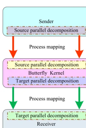
communication load among processes is balanced, and that the number of processes must be a power of 2. In practice, data transfer for model coupling has different characteristics: one process needs to communicate with a part of other pro-cesses, the communication load among processes is always unbalanced, and the number of processes cannot be restricted to a power of 2. Therefore, we propose here a new implemen-tation of data transfer involving an additional butterfly kernel to transfer data from the sender with the source parallel de-composition to the receiver with the target parallel decom-position. As the number of processes of the butterfly kernel must be a power of 2, while the number of processes of the sender or the receiver are not necessarily, the butterfly kernel has its own source and target parallel decompositions, and process mappings are required from the sender onto the but-terfly kernel and from the butbut-terfly kernel onto the receiver (see Fig. 7). Next, we present the butterfly kernel and the process mappings.
3.1 Butterfly kernel
The first question for the butterfly kernel is how to decide its number of processes. Any process of the sender or receiver can be used as a process for the butterfly kernel. Given that the total number of unique processes of the sender and re-ceiver isNT, the number of processes of the butterfly kernel (NB)can be any power of 2, which is no larger thanNT. We propose to select the maximum number in order to maximize utilization of resources. We prefer to pick out unique pro-cesses first from the sender, and then from the receiver if the sender does not have enough processes.
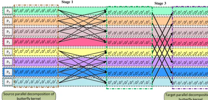
Figure 6.An example of the butterfly kernel with eight processes. Each coloured row stands for one process (P0–P7). There are multiple
stages (each column of arrows represents a stage (stage 1 to stage 3)) in the butterfly kernel. Each arrow stands for an MPI P2P communication from one process to another.Dji means the data are originally in processPiaccording to the source parallel decomposition and is finally in processPjaccording to the target parallel decomposition.
Figure 7.The butterfly implementation, which is composed of three parts: the butterfly kernel, process mapping from the sender to the butterfly kernel, and process mapping from the butterfly kernel to the receiver.
butterfly kernel. In a stage, all processes are divided into a number of pairs and the two processes of a pair use MPI P2P communication to exchange data. After each stage, the num-ber of butterfly kernel processes that may have the data that will finally belong to any one process on the target parallel decomposition will become a half. Figure 6 is an example for further illustration, where Dij means the data are originally in processPi according to the source parallel decomposition
and are finally in processPj according to the target parallel
decomposition. Before the first stage, all processes (P0–P7)
may have the data ofP0on the target parallel decomposition. After the first stage, only four processes (P0,P2,P4, andP6) may have that data; and after the second stage, only two pro-cesses (P0andP4)may have it.
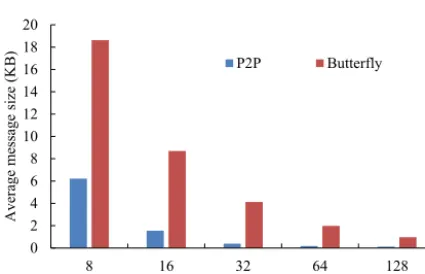
To reveal the advantages and disadvantages of the two implementations, we measure the characteristics of the two implementations based on the benchmark introduced in Sect. 2.2. The results show that the total amount of data transferred by the butterfly implementation is larger than that transferred by the P2P implementation (Fig. 8), which is the major disadvantage of the butterfly implementation. Mean-while, compared with the P2P implementation, the butterfly implementation can have the following advantages:
1. bigger message size for better communication band-width (Fig. 9);
2. balanced and smaller number of MPI processes among processes (Fig. 10);
3. ordered communications among processes and fewer communications operated concurrently (Fig. 10), which can dramatically reduce network contention.
3.2 Process mapping
0 20 40 60 80 100 120 140 160 180 200 220
8 16 32 64 128
T o ta l am o u n t o f d at a tr an sf er re d ( K B )
Number of processes per model
P2P Butterfly
Figure 8.Total amount of data transferred by P2P implementation and butterfly implementation (y axis) in GAMIL2–CLM3, when varying the number of processes per model (x axis). The experi-mental set-up is similar to that shown in Fig. 1.
0 2 4 6 8 10 12 14 16 18 20
8 16 32 64 128
Aver ag e m ess age si ze (KB )
Number of processes per model
P2P Butterfly
Figure 9.Average message size transferred by P2P implementation and butterfly implementation (y axis) in GAMIL2–CLM3, when varying the number of processes per model (x axis). The experi-mental set-up is similar to that shown in Fig. 1.
In other words, there is no multiple-to-multiple process map-ping between the butterfly kernel and the receiver. Similarly, there is no multiple-to-multiple process mapping between the sender and the butterfly kernel.
Processes of the sender or the receiver may be unbalanced in terms of the data size transferred, which may result in un-balanced communications among processes of the butterfly kernel. As mentioned in Sect. 3.1, at each stage of the butter-fly kernel, all processes are divided into a number of pairs, each of which is involved in P2P communications. To im-prove the balance of communications among the processes in the butterfly kernel, one solution is to try to make the pro-cess pairs at each stage more balanced in terms of the data size of P2P communications, so we propose to reorder the processes of the sender or the receiver according to data size. At the first stage, we pick out the process with the largest data size and the process with the smallest data size from the remaining processes that have not been paired, to generate a process group. For the next stage, the outputs of two pro-cess groups from the previous stage are paired into bigger
1 2 4 8 16 32 64
8 16 32 64 128
N um b er of M PI m ess age s
Number of processes per model Maximum of P2P Average of P2P Minimum P2P Maximum of butterfly Average of butterfly Minimum of butterfly
Figure 10.Maximum number of MPI messages, average number of MPI messages and minimum MPI messages in P2P implementation and butterfly implementation (yaxis), when varying the number of processes per model (xaxis) in GAMIL2–CLM3. The experimental set-up is similar to that shown in Fig. 1.
process groups in a similar way. After finishing the iterative pairing throughout all stages, all processes of the sender or the receiver are reordered.
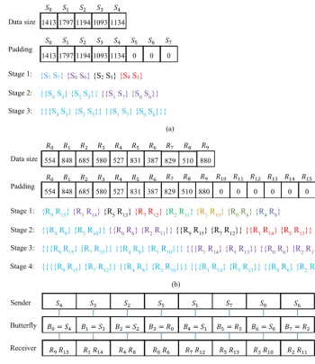
The iterative pairing also requires the number of processes to be a power of 2. Given that the number of processes of the sender (or receiver) isNCand the number of processes of the butterfly kernel isNB, we first pad empty processes (whose data size is zero) before the iterative pairing to make the num-ber of processes of the sender (or receiver) be a power of 2 (donatedNP), which is no smaller thanNB. Therefore, the reorderedNPprocesses after the iterative pairing can be di-vided intoNB groups, each of which containsNP/NB pro-cesses with consecutive reordered indexes and maps onto a unique process of the butterfly kernel.
Figure 11 shows an example of the process mapping, where the sender has 5 processes (S0–S4 in Fig. 11a), the receiver has 10 processes (R0–R9in Fig. 11b), and the but-terfly kernel uses 8 processes (B0–B7in Fig. 11c). At first, empty processes are padded to the sender (S5–S7in Fig. 11a) and the receiver (R10–R15 in Fig. 11b). Next, the itera-tive pairing is conducted for the sender and the receiver. The iterative pairing has three stages for the sender. At the first stage, the eight processes of the sender are divided into four groups {S1, S7}, {S0, S6}, {S2, S5}, and {S4, S3}
(Fig. 11a), according to the data size corresponding to each process. These four process groups are divided into two bigger groups {{S4, S3},{S2, S5}} and {{S1, S7},{S0, S6}} at the second stage (Fig. 11a). Finally, one process group
Figure 11.An example of process mappings, given that the sender has 5 processes (S0–S4), the receiver has 10 processes (R0–R9)(there is
no common process between the sender and receiver), and the butterfly kernel contains 8 processes (B0–B7). Panels(a)and(b)show how to
iteratively pair processes of the sender and receiver, respectively. There are multiple stages in the iterative pairing of processes of the sender and receiver. In each stage, the processes in the same colour are grouped into one process pair. Panel(c)shows how to map the reordered processes of the sender and receiver onto the processes of the butterfly kernel.
(Fig. 11c). Similarly, the iterative pairing has four stages for the receiver, and the 16 processes of the receiver are re-ordered asR9,R15,R7,R12,R4,R8,R3,R10,R1,R14,R5,
R13,R0,R6,R2, andR11, with pairs of these being mapped onto 1 process of the butterfly kernel (Fig. 11c).
4 Adaptive data transfer library
Now, we have two kinds of implementations (the P2P imple-mentation and the butterfly impleimple-mentation) for data transfer. Although the butterfly implementation can effectively im-prove the performance of data transfer in many cases (ex-amples are given in Sect. 5), it has some drawbacks: (1) it
generally has a larger total amount of data transferred than the P2P implementation; (2) its number of stages is log2N
(whereNis the number of processes for the butterfly kernel) (Foster, 1995), which may be bigger than the average number of MPI messages in the P2P implementation in some cases (for example, when the sender and the receiver use the simi-lar parallel decompositions). Therefore, it is possible that the P2P implementation outperforms the butterfly implementa-tion in some cases. To achieve optimal performance for data transfer, we propose an adaptive data transfer library that can take the advantages of the two implementations in all cases.
Figure 12.An example of the adaptive data transfer library with eight processes, where stage 2 of the butterfly implementation is skipped and replaced by P2P communication of three MPI messages per process.
one MPI message per process. Inspired by this fact, we try to design an adaptive approach that can combine the butterfly and P2P implementations, where some stages in the butterfly implementation are skipped and replaced by P2P communi-cation of more MPI messages per process. When all stages of the butterfly implementation are skipped, the adaptive data transfer library completely switches to the original P2P im-plementation. That is to say, the adaptive data transfer can adaptively choose the optimal implementation from the P2P implementation and the butterfly implementation. Figure 12 shows an example of the adaptive data transfer library with eight processes, where stage 2 of the butterfly implementa-tion is skipped and replaced by P2P communicaimplementa-tion of three MPI messages per process.
The most significant challenge of such an adaptive ap-proach is to determine which stage(s) of the butterfly imple-mentation should be skipped. The first attempt was to design a cost model that can accurately predict the performance of data transfer in various implementations. We eventually gave up this approach as it was almost impossible to accurately predict the performance of the communications on a high-performance computer, especially when a lot of users share the computer to run various applications. Performance profil-ing, which means directly measuring the performance of data transfer, is more practical to determine an appropriate imple-mentation, because the simulation of Earth system modelling always takes a long time to run. Figure 13 shows our flow chart of how the adaptive data transfer library determines an appropriate implementation. It consists of an initialization segment and a profiling segment. The initialization segment generates the process mappings and a candidate implementa-tion that is a butterfly implementaimplementa-tion with no skipped stages. The profiling segment iterates through each stage of the but-terfly implementation to determine whether the current stage should be skipped or kept. In an iteration, the profiling seg-ment first generates a temporary impleseg-mentation based on the
candidate implementation where the current stage is skipped, and then runs the temporary implementation to get the time the data transfer takes. When the temporary implementation is more efficient than the candidate implementation, the cur-rent stage is skipped and the temporary implementation re-places the candidate implementation. When the profiling seg-ment finishes, the appropriate impleseg-mentation is set to be the candidate implementation. To reduce the overhead in-troduced by the adaptive data transfer library, the profiling segment truly transfers the data for model coupling. In other words, before obtaining an optimal implementation, the data is transferred by the profiling segment.
5 Performance evaluation
In this section, we empirically evaluate the adaptive data transfer library, through comparing it to the P2P imple-mentation and the butterfly impleimple-mentation. Both toy mod-els and realistic modmod-els (GAMIL2–CLM3 and CESM – Community Earth System Model) are used for the perfor-mance evaluation. GAMIL2–CLM3 has been introduced in Sect. 2.2. CESM (Hurrell et al., 2013) is a state-of-the-art ESM developed by the National Center for Atmospheric Re-search (NCAR). All the experiments are run on the high-performance computer Tansuo100.
Next, we will evaluate the overhead of initialization, the performance of transferring data fields between two toy mod-els and between different realistic component modmod-els, and the performance of rearranging data fields within a compo-nent model for parallel interpolation.
5.1 Overhead of initialization
increas-Figure 13.A flow chart for determining an appropriate implemen-tation of the adaptive data transfer library.
ing the number of processes. The initialization overhead of the butterfly implementation is a little higher than that of the P2P implementation, while the initialization overhead of the adaptive data transfer library is 2–3-fold higher than that of the P2P implementation, because the adaptive data trans-fer library uses extra time on the performance profiling (see Sect. 4). Considering that one data transfer instance should only be initialized at the beginning and executed many times in a coupled model, we can conclude that the initialization overhead of the adaptive data transfer library is reasonable, especially when the simulation is executed for a very long time.
5.2 Performance of data transfer between toy models
The factors that can impact the performance of a data transfer implementation generally include the number of MPI mes-sages, the size of the data to be transferred (also referred to as the number of fields in this evaluation) and the number of processes used. In this subsection, we evaluate the impact of each factor on the performance of data transfer for different implementations. We first build two toy models that both use the same logically rectangular grid of 192×480 grid points. Coupling fields are transferred between the two toy models. For any test, the two toy models use the same number of pro-cesses. Next, we evaluate the performance of data transfer through varying one factor while fixing the other two factors.
Figure 14.Initialization time (yaxis) of one data transfer between two toy models using a rectangular grid (of 192×96 grid points) when varying the number of processes per model (xaxis). There are 10 2-D coupling fields transferred from the source toy model to the target toy model. In each test, all processes of the sender in the P2P implementation have the same number of MPI messages. If the number of processes per model is less than 24, the number of MPI messages per sender process in the P2P implementation is equal to the number of processes per model; otherwise, the number of MPI messages per sender process in the P2P implementation is 24. The parallel decompositions of the sender and the receiver for a given average number of MPI messages are generated by Algorithm 1.
0 0.002 0.004 0.006 0.008 0.01 0.012 0.014
1 3 6 12 24 48 90
T
im
e
(s
)
Number of MPI messages per sender process in the P2P implementation Adaptive
P2P Butterfly
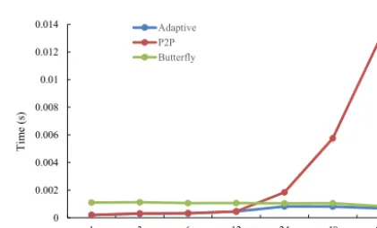
Figure 15.Average execution time (yaxis) of one data transfer be-tween two toy models with the same rectangular grid (of 192×480 grid points) when varying the number of MPI messages per sender process in the P2P implementation (xaxis). Each toy model is run with 1024 processes. There are 10 2-D coupling fields transferred from the source toy model to the target toy model.
implemen-21 1
Algorithm 1. Generating the parallel decompositions of the sender and the receiver according to an average number of MPI messages of the sender in the P2P implementation.
Input Number of processes of the sender: M Number of processes of the receiver: N Number of points in the grid: Grid_pnts
Average number of MPI messages per process of the sender in the P2P implementation: Avg_send_msgs, Avg_send_msgs ≤ N
The flag that specifies whether the number of MPI messages among processes are the same: Is_balanced
Output Parallel decomposition of the sender Parallel decomposition of the receiver
1 Determine the parallel decomposition of the sender
Considering that the numbers of grid points are always balanced among the processes of a model, assign around Grid_pnts/M grid points to each process of the sender.
2 Determine the number of MPI messages of each process of the sender
2.1 If the flag Is_balanced is set to true, set the number of MPI messages of each process of the sender to be Avg_send_msgs;
2.2 Otherwise, randomly determine the number of MPI messages of each process of the sender 2.2.1 Initialize the number of MPI messages of each process of the sender to be 1
2.2.2 Randomly select a process of the sender whose number of MPI messages does not exceed N and Grid_pnts/M, and then increase its number of MPI messages by 1, until the average number of MPI messages of all processes of the sender reaches Avg_send_msgs.
3 Determine the grid points of each MPI message
For each process of the sender, assign the corresponding grid points to all MPI messages of this process (a grid point belongs to only one MPI message)
3.1 If the flag Is_balanced is set to true, assign the grid points to all MPI messages evenly. 3.2 Otherwise, assign the grid points to each MPI message randomly
3.2.1 Assign one grid point to each MPI message
3.2.2 For each of remaining grid points, randomly select an MPI message for it
4 Determine the parallel decomposition of the receiver through assigning the grid points in each MPI message to a process of the receiver
For each process of the sender, assign the grid points in each MPI message of it to a distinct receiver process: to make the numbers of grid points balance among the processes of the receiver in the final parallel decomposition, an MPI message with bigger number of grid points will be assigned to a receiver process with smaller total number of grid points that have been assigned to it.
2
tations when increasing the number of MPI messages per sender process in the P2P implementation from 1 to 90. The P2P implementation can outperform the butterfly imple-mentation when the number of MPI messages is small (e.g. smaller than 12 in Fig. 15), while the butterfly implementa-tion can outperform the P2P implementaimplementa-tion when the num-ber of MPI messages is big (e.g. bigger than 12 in Fig. 15). The adaptive data transfer library can adaptively choose the optimal implementation from the P2P implementation and the butterfly implementation and, moreover, it improves the performance based on the butterfly implementation when the number of MPI messages is big, since some butterfly stages of the butterfly implementation are skipped. When the
num-ber of MPI messages is 90, the adaptive data transfer library can achieve a 19.2-fold performance speed-up compared to the P2P implementation.
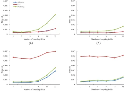
im-Figure 16.Average execution time (yaxis) of one data transfer between two toy models with the same rectangular grid (of 192×480 grid points) when varying the number of coupling fields transferred (xaxis). There are four simulation tests for the evaluation. In simulation(a), each toy model is run with 256 processes, and the number of MPI messages per sender process in the P2P implementation is 12. In simu-lation(b), each toy model is run with 1024 processes, and the number of MPI messages per sender process is in the P2P implementation 12. In simulation(c), each toy model is run with 256 processes, and the number of MPI messages per sender process in the P2P implemen-tation is 48. In simulation(d), each toy model is run with 1024 processes, and the number of MPI messages per sender process in the P2P implementation is 48.
plementation, especially when the number of 2-D coupling fields gets bigger. When the number of MPI messages per sender process in the P2P implementation is big (Fig. 16c, d), the butterfly implementation significantly outperforms the P2P implementation; however, the advantage of the butter-fly implementation decreases when increasing the number of coupling fields. The results also demonstrate that the adap-tive data transfer library can adapadap-tively choose the optimal implementation from the P2P implementation and the butter-fly implementation, and can further improve the performance based on the butterfly implementation.
In the third experiment, we fix the number of MPI mes-sages per sender process in the P2P implementation to be 24 and the number of coupling fields transferred to be 10, and vary the number of processes used. Figure 17 shows the ex-ecution time of one data transfer with different implementa-tions when varying the number of processes. The P2P imple-mentation outperforms the butterfly impleimple-mentation when a small number of processes are used (e.g. smaller than 256 in Fig. 17), while the butterfly implementation outperforms the
P2P implementation when a large number of processes are used (e.g. larger than 256 in Fig. 17). Similar to the above two experiments, the adaptive data transfer library can adap-tively choose the optimal implementation from the P2P im-plementation and the butterfly imim-plementation.
0 0.0005 0.001 0.0015 0.002 0.0025 0.003 0.0035
192 256 384 512 768 1024
T
im
e (
s)
Number of processes per model
Adaptive P2P Butterfly
Figure 17. Average execution time (y axis) of one data trans-fer between two toy models with the same rectangular grid (of 192×480 grid points) when varying the number of processes per model (xaxis). There are 10 2-D coupling fields transferred from the source toy model to the target toy model. In each test, the num-ber of MPI messages per sender process in the P2P implementation is 24.
0 0.001 0.002 0.003 0.004 0.005 0.006 0.007
64 96 128 192 256 384 512 768 1024
T
im
e (
s)
Number of processes per model Adaptive
P2P Butterfly
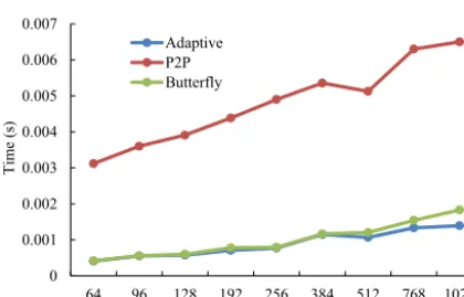
Figure 18.Average execution time (yaxis) of one data transfer be-tween two toy models. In this evaluation, each process (running on a unique processor core) of the toy models has 96 grid points, while different processes have a different number of MPI messages and different message sizes in the P2P implementation. The number of coupling fields transferred is set to 20.
(from 64 to 1024), the butterfly implementation significantly outperforms the P2P implementation. So the adaptive data transfer library adaptively chooses the butterfly implemen-tation, and further slightly outperforms the butterfly imple-mentation when each model uses more than 512 processes because some butterfly stages are skipped.
5.3 Performance of data transfer between realistic models
In this subsection, we evaluate the performance using two realistic models: GAMIL2–CLM3 (horizontal resolution of 2.8◦×2.8◦) and CESM (resolution of 1.9x2.5_gx1v6).
0 0.0005 0.001 0.0015 0.002 0.0025
6 12 24 48 96 192
T
im
e (
s)
Number of processes per model Adaptive P2P Butterfly
Figure 19.Average execution time (y axis) of one data transfer between the land surface model CLM4 and the coupler CPL7 in CESM when varying the number of processes per model (xaxis): 32 coupling fields on the CLM horizontal grid (the grid size is 144×96=13 824) are transferred from the land surface model CLM4 to the coupler CPL7. The performance results of the P2P im-plementation are obtained through running the adaptive data trans-fer library forcing it to completely switch to the original P2P imple-mentation.
For CESM, we use the data transfer between the coupler CPL7 (Craig et al., 2012) and the land surface model CLM4 (Oleson et al., 2004), where 32 2-D coupling fields on the CLM4 horizontal grid (the grid size is 144×96=13 824) are transferred. Figure 19 shows the performance of one data transfer of different implementations when increasing the number of processes of both CPL7 and CLM4 from 6 to 192. When the number of processes is small (e.g. smaller than 24 in Fig. 19), the butterfly implementation is much poorer than the P2P implementation. In this case, the adap-tive data transfer library chooses the P2P implementation as the optimal implementation. However, when the number of processes gets bigger (e.g. larger than 24 in Fig. 19), the butterfly implementation outperforms the P2P implementa-tion. In this case, the adaptive data transfer library, based on the butterfly implementation, skips some stages, outperform-ing the butterfly implementation. Figure 19 also shows that the butterfly implementation and the adaptive transfer library seem to converge when increasing the number of processes per model. When each model uses 192 processes, the adap-tive data transfer library is 4.01 times faster than the P2P implementation.
adap-Figure 20.Average execution time (yaxis) of one data transfer be-tween the atmosphere model GAMIL2 and the land surface model CLM3 in GAMIL2–CLM3 when varying the number of processes per model (xaxis): 14 coupling fields on the GAMIL2 horizontal grid (the grid size is 128×60=7680) are transferred from the land surface model CLM3 to the atmosphere model GAMIL2.
tive data transfer library achieves an 11.68-fold performance speed-up when the number of processes is 96, but achieves a much lower speed-up (only 3.48-fold) when the number of processes is 192. This is because the average number of MPI messages per process in the P2P implementation re-duces from 32 to 18 when the number of process increases from 96 to 192.
5.4 Performance of data rearrangement for interpolation
Besides data transfer between different component models, there is another kind of data transfer in model coupling that rearranges data inside a model for parallel interpolation of fields between different grids. Here, we use the data rear-rangement for the parallel interpolation from the atmosphere grid (whose grid size is 144×96=13 824) to the ocean grid (whose grid size is 320×384=122 880) in the coupled model CESM for further evaluation. As shown on Fig. 21, the P2P implementation significantly outperforms the butter-fly implementation. This is because the parallel decomposi-tions before and after data rearrangement are always similar, which leads to small number of MPI messages. For example, the average number of MPI messages in the P2P implemen-tation corresponding to Fig. 21 is only 6.49 when the model uses 96 processes. In this case, the P2P implementation is chosen as the optimal implementation of the data transfer li-brary, so the data transfer library does not provide real benefit compared to the P2P implementation.
5.5 Performance improvement for a coupled model
With the performance improvement of data transfer, we ex-pect that the adaptive data transfer library will improve the performance of coupled models. For this evaluation, we first
Figure 21.Average execution time (yaxis) of one data rearrange-ment for the parallel interpolation from the atmosphere grid (the grid size is 144×96=13 824) to the ocean grid (the grid size is 320×384=122 880) in CESM when varying the number of pro-cesses per model (xaxis).
0.9 0.92 0.94 0.96 0.98 1 1.02 1.04 1.06 1.08 1.1
6 8 12 16 24 32 48 64 96 128
Sp
eedup
Number of processes per model Speedup achieved by the adaptive data transfer library
Speedup achieved by the butterfly implementation
Figure 22. Performance improvement with respect to the whole model time for the coupled model GAMIL2–CLM3 achieved by the butterfly implementation and the adaptive data transfer library, using the P2P implementation as the baseline.
imported the adaptive data transfer library into C-Coupler1, used it in the coupled model GAMIL2–CLM3, and measured performance results. As shown in Fig. 22, the adaptive data transfer library achieves higher speed-up with respect to the whole model time (when the P2P implementation is used as the baseline) for GAMIL2–CLM3 when using more than 16 processes. When each component model uses 128 pro-cesses, the butterfly implementation achieves ∼4.6 % per-formance improvement, and the adaptive data transfer library achieves∼6.9 % performance improvement. Therefore, the data transfer library can improve the performance of data transfer, and then improve the performance of the whole cou-pled model.
6 Conclusions
imple-mentation currently used in most state-of-the-art couplers for data transfer is inefficient when the parallel decompo-sitions of the sender and the receiver are different, and fur-ther revealed the corresponding performance bottlenecks. We showed that the butterfly implementation can outperform the P2P implementation in many cases but degrades the perfor-mance in some cases, for example when a small number of processes are used to run models or when the parallel decom-positions of the sender and receiver are similar. We therefore designed and implemented an adaptive data transfer library that automatically chooses an optimal implementation be-tween the P2P implementation and the butterfly implemen-tation and also further improves the performance based on the butterfly implementation through skipping some butter-fly stages. Compared to the P2P implementation, the adap-tive data transfer library can improve the performance of data transfer when the parallel decompositions of the sender and the receiver are different.
The initialization overhead for the adaptive data transfer library could become expensive when using a large number of processes. In the future version, the adaptive data transfer will allow users to record the results of performance profiling offline to save the time used for performance profiling in the next run of the same coupled model.
Code availability
The source code of the adaptive data transfer library version 1.0 is available at https://github.com/zhang-cheng09/Data_ transfer_lib.
Acknowledgements. This work is supported in part by the
Natural Science Foundation of China (no. 41275098), the Na-tional Grand Fundamental Research 973 Program of China (no. 2013CB956603), and the Tsinghua University Initiative Scientific Research Program (no. 20131089356).
Edited by: S. Valcke
References
Armstrong, C. W., Ford, R. W., and Riley, G. D.: Coupling inte-grated Earth System Model components with BFG2, Concur-rency and Computation: Practice and Experience, 21, 767–791, doi:10.1002/cpe.1348, 2009.
Balaji, V., Anderson, J., Held, I., Winton, M., Durachta, J., Maly-shev, S., and Stouffer, R. J.: The Exchange Grid: a mechanism for data exchange between Earth system components on indepen-dent grids, in: Parallel Computational Fluid Dynamics 2005 The-ory and Applications, 179–186, doi:10.1016/B978-044452206-1/50021-5, 2006.
Chong, F. T. and Brewer, E. A.: Packaging and multiplexing of hierarchical scalable expanders, Parallel Computer Routing and Communication, Springer Berlin Heidelberg, 200–214, 1994.
Craig, A. P., Jacob, R., Kauffman, B., Bettge, T., Larson, J., Ong, E., Ding, C., and He, Y.: CPL6: the New Extensible, High Per-formance Parallel Coupler for the Community Climate System Model, Int. J. High Perform. C., 19, 309–327, 2005.
Craig, A. P., Vertenstein, M., and Jacob, R.: A new flex-ible coupler for Earth system modelling developed for CCSM4 and CESM1, Int. J. High Perform. C., 26, 31–42, doi:10.1177/1094342011428141, 2012.
Dennis, J. M.: Inverse space-filling curve partitioning of a global ocean model, in: IEEE International Parallel & Distributed Pro-cessing Symposium, Long Beach, CA, 2007.
Dennis, J. M. and Tufo, H. M.: Scaling climate simulation appli-cations on the IBM Blue Gene/L system, IBM J. Res. Dev., 52, 117–126, doi:10.1147/rd.521.0117, 2008.
Dennis, J. M., Edwards, J., Evans, K. J., Guba, O., Lauritzen, P. H., Mirin, A. A., St-Cyr, A., Taylor, M. A., and Worley, P. H.: CAM-SE: a scalable spectral element dynamical core for the Commu-nity Atmosphere Model, Int. J. High Perform. C., 26, 74–89, doi:10.1177/1094342011428142, 2012.
Dickinson, R. E., Oleson, K. W., Bonan, G., Hoffman, F., Thornton, P., Vertenstein, M., Yang, Z.-L., and Zeng, X.: The Community Land surface model and its climate statistics as a component of the Community Climate System Model, J. Climate, 19, 2302– 2324, 2006.
Ford, R. W., Riley, G. D., Bane, M. K., Armstrong, C. W., and Free-man, T. L.: GCF: a general coupling framework, Concurr. Comp. Pract. E., 18, 163–181, 2006.
Foster, I.: Designing and building parallel programs: concepts and tools for parallel software engineering, Addison-Wesley, 1995. Heckbert P.: Fourier Transforms and the Fast Fourier Transform
(FFT) Algorithm, Comp. Graph., 2, 15–463, 1995.
Hemmert, K. S. and Underwood, K. D.: An analysis of the double-precision floating-point FFT on FPGAs, Field-Programmable Custom Computing Machines, 2005, FCCM 2005, 13th Annual IEEE Symposium on IEEE, 171–180, 2005.
Hill, C., DeLuca, C., Balaji, V., Suarez, M., and da Silva, A.: The Architecture of the Earth System Modelling Framework, Com-put. Sci. Eng., 6, 18–28, 2004.
Hurrell, J. W., Holland, M. M., Gent, P. R., Ghan, S., Kay, J. E., Kushner, P. J., Lamarque, J.-F., Large, W. G., Lawrence, D., Lindsay, K., Lipscomb, W. H., Long, M. C., Mahowald, N., Marsh, D. R., Neale, R. B., Rasch, P., Vavrus, S., Vertenstein, M., Bader, D., Collins, W. D., Hack, J. J., Kiehl, J., and Mar-shall, S.: The Community Earth System Model: a framework for collaborative research, B. Am. Meteorol. Soc., 94, 1339–1360, 2013.
Hunke, E. C. and Lipscomb W. H.: CICE: the Los Alamos Sea Ice Model Documentation and Software User’s Manual 4.0, Techni-cal Report LA-CC-06-012, Los Alamos National Laboratory, T-3 Fluid Dynamics Group, 2008.
Hunke, E. C., Lipscomb, W. H., Turner, A. K., Jeffery, N., and Elliott, S.: CICE: the Los Alamos Sea Ice Model Documenta-tion and Software User’s Manual Version 5.0, LA-CC-06-012, Los Alamos National Laboratory, Los Alamos NM, 87545, 115, 2013.
doi:10.1007/s00376-013-2157-5, 2013.
Liu, L., Yang, G., Wang, B., Zhang, C., Li, R., Zhang, Z., Ji, Y., and Wang, L.: C-Coupler1: a Chinese community coupler for Earth system modeling, Geosci. Model Dev., 7, 2281–2302, doi:10.5194/gmd-7-2281-2014, 2014.
Morrison, H. and Gettelman, A.: A new two-moment bulk strati-form cloud microphysics scheme in the Community Atmosphere Model, version 3 (CAM3). Part I: Description and numerical tests, J. Climate, 21, 3642–3659, doi:10.1175/2008JCLI2105.1, 2008.
Neale, R. B., Richter, J. H., Conley, A. J., Park, S., Lauritzen, P. H., Gettelman, A., Williamson, D. L., Rasch, P. J., Vavrus, S. J., Taylor, M. A., Collins, W. D., Zhang, M., and Lin, S.: Descrip-tion of the NCAR Community Atmosphere Model (CAM 4.0), National Center for Atmospheric Research Ncar Koha Opencat, TN-485+STR, 222 pp., 2010.
Neale, R. B., Chen, C. C., Gettelman, A., Lauritzen, P. H., Park, S., Williamson, D. L., Conley, A. J., Garcia, R., Kinnison, D., Lamarque, J. F., Marsh, D., Mills, M., Smith, A. K., Tilmes, S., Vitt, F., Morrison, H., Cameron-Smith, P., Collins, W. D., Iacono, M. J., Easter, R. C., Ghan, S. J., Liu, X., Rasch, P. J., and Tay-lor, M. A.: Description of the NCAR Community Atmosphere Model (CAM 5.0), National Center for Atmospheric Research Ncar Koha Opencat, TN-486+STR, 289 pp., 2012.
Smith, R., Jones, P., Briegleb, B., Bryan, F., Danabasoglu, G., Den-nis, J., Dukowicz, J., Eden, C., Fox-Kemper, B., Gent, P., Hecht, M., Jayne, S., Jochum, M., Large, W., Lindsay, K., Maltrud, M., Norton, N., Peacock, S., Vertenstein, M., and Yeager, S.: The Par-allel Ocean Program (POP) reference manual ocean component of the Community Climate System Model (CCSM) and Commu-nity Earth System Model (CESM), Los Alamos National Lab-oratory, LAUR-10-01853, available at: http://www.cesm.ucar. edu/models/cesm1.1/pop2/doc/sci/POPRefManual.pdf (last ac-cess: 15 October 2015), 141 pp., 2010.
Valcke, S., Balaji, V., Craig, A., DeLuca, C., Dunlap, R., Ford, R. W., Jacob, R., Larson, J., O’Kuinghttons, R., Riley, G. D., and Vertenstein, M.: Coupling technologies for Earth System Mod-elling, Geosci. Model Dev., 5, 1589–1596, doi:10.5194/gmd-5-1589-2012, 2012.
Valcke, S.: The OASIS3 coupler: a European climate mod-elling community software, Geosci. Model Dev., 6, 373–388, doi:10.5194/gmd-6-373-2013, 2013.