https://doi.org/10.5194/essd-9-881-2017 © Author(s) 2017. This work is distributed under the Creative Commons Attribution 3.0 License.
Cloud property datasets retrieved from AVHRR,
MODIS, AATSR and MERIS in the framework
of the Cloud_cci project
Martin Stengel1, Stefan Stapelberg1, Oliver Sus1, Cornelia Schlundt1, Caroline Poulsen2, Gareth Thomas2, Matthew Christensen2, Cintia Carbajal Henken3, Rene Preusker3, Jürgen Fischer3,
Abhay Devasthale4, Ulrika Willén4, Karl-Göran Karlsson4, Gregory R. McGarragh5, Simon Proud5, Adam C. Povey6, Roy G. Grainger6, Jan Fokke Meirink7, Artem Feofilov8, Ralf Bennartz9,10,
Jedrzej S. Bojanowski11, and Rainer Hollmann1
1Deutscher Wetterdienst, Frankfurter Str. 135, 63067 Offenbach, Germany 2Rutherford Appleton Laboratory, Didcot, Oxfordshire, UK
3Institute for Space Sciences, Freie Universität Berlin, Carl-Heinrich-Becker-Weg 6–10, 12165 Berlin, Germany
4Swedish Meteorological and Hydrological Institute (SMHI), Norrköping, Sweden
5Department of Physics, University of Oxford, Clarendon Laboratory, Parks Road, Oxford OX1 3PU, UK 6National Centre for Earth Observation, University of Oxford, Oxford, OX1 3PU, UK
7Royal Netherlands Meteorological Institute (KNMI), De Bilt, the Netherlands 8Laboratoire de météorologie dynamique (LMD), Paris, France
9University of Wisconsin, Madison, Wisconsin, USA 10Vanderbilt University, Nashville, Tennessee, USA
11MeteoSwiss, Zurich, Switzerland
Correspondence to:Martin Stengel ([email protected])
Received: 6 June 2017 – Discussion started: 20 June 2017
Revised: 26 September 2017 – Accepted: 5 October 2017 – Published: 23 November 2017
Abstract. New cloud property datasets based on measurements from the passive imaging satellite sensors
AVHRR, MODIS, ATSR2, AATSR and MERIS are presented. Two retrieval systems were developed that in-clude components for cloud detection and cloud typing followed by cloud property retrievals based on the optimal estimation (OE) technique. The OE-based retrievals are applied to simultaneously retrieve cloud-top pressure, cloud particle effective radius and cloud optical thickness using measurements at visible, near-infrared and thermal infrared wavelengths, which ensures spectral consistency. The retrieved cloud properties are fur-ther processed to derive cloud-top height, cloud-top temperature, cloud liquid water path, cloud ice water path and spectral cloud albedo. The Cloud_cci products are pixel-based retrievals, daily composites of those on a global equal-angle latitude–longitude grid, and monthly cloud properties such as averages, standard deviations and histograms, also on a global grid. All products include rigorous propagation of the retrieval and sampling uncertainties. Grouping the orbital properties of the sensor families, six datasets have been defined, which are
named AVHRR-AM, AVHRR-PM, MODIS-Terra, MODIS-Aqua, ATSR2-AATSR and MERIS+AATSR, each
uncertainty propagation through all processing levels can be considered as new features of the Cloud_cci datasets compared to existing datasets. In addition, the consistency among the individual datasets allows for a potential combination of them as well as facilitates studies on the impact of temporal sampling and spatial resolution on cloud climatologies.
For each dataset a digital object identifier has been issued:
Cloud_cci AVHRR-AM: https://doi.org/10.5676/DWD/ESA_Cloud_cci/AVHRR-AM/V002 Cloud_cci AVHRR-PM: https://doi.org/10.5676/DWD/ESA_Cloud_cci/AVHRR-PM/V002 Cloud_cci MODIS-Terra: https://doi.org/10.5676/DWD/ESA_Cloud_cci/MODIS-Terra/V002 Cloud_cci MODIS-Aqua: https://doi.org/10.5676/DWD/ESA_Cloud_cci/MODIS-Aqua/V002 Cloud_cci ATSR2-AATSR: https://doi.org/10.5676/DWD/ESA_Cloud_cci/ATSR2-AATSR/V002 Cloud_cci MERIS+AATSR: https://doi.org/10.5676/DWD/ESA_Cloud_cci/MERIS+AATSR/V002
1 Introduction
Satellite-based datasets of geophysical variables are crucial for climate research as they represent observations of the Earth’s climate system, which can be used for both the analy-sis of the climate and its variability as well as guidance for at-mospheric model developments. These datasets evolve peri-odically by mainly two activities: (1) extending and improv-ing the underlyimprov-ing radiance record by addimprov-ing new satellite recordings and applying new inter-calibration to the entire record, and (2) the development and application of more ad-vanced retrieval systems and the utilization of additional or more frequent auxiliary data which often undergo regular up-dates themselves.
In the last few decades, activities to process and reprocess global, high-quality cloud property datasets based on long-term satellite measurement records have been undertaken with increased effort. The backbone of most of the multi-decadal climate datasets of cloud properties has been the National Oceanic and Atmospheric Administration (NOAA) Polar Operational Environmental Satellites (POES) series. The Advanced Very High Resolution Radiometer (AVHRR) has been on board the NOAA satellites since the end of the 1970s (i.e. NOAA-5 and beyond). AVHRR is a passive imaging sensor, where the source of measured radiation is not emitted by the instrument. Instead, the upwards reflected solar and emitted thermal radiation is measured at the top of the atmosphere (TOA). This is done in abutting pixels that assemble a seamless image. With its four to six spec-tral channels, AVHRR allows the retrieval of key cloud prop-erties. AVHRR has been a significant contributor to many global cloud climatologies, e.g. the International Satellite Cloud Climatology Project (ISCCP; Schiffer and Rossow, 1983; Rossow and Schiffer, 1999), the Pathfinder extended dataset (PATMOS-x; Heidinger et al., 2014) and the Cli-mate Monitoring Satellite Application Facility’s (CM SAF) cloud, albedo and radiation dataset (CLARA-A1/A2; Karls-son et al., 2013, 2016).
Since the 1990s the National Aeronautics and Space Ad-ministration (NASA) and the European Space Agency (ESA)
have launched research satellite missions, e.g. Terra, Aqua, the European Remote Sensing Satellite (ERS-1/2) and the Environmental Satellite (Envisat), that carry AVHRR her-itage sensors. These are the Moderate Resolution Imaging Spectroradiometer (MODIS), the Along-Track Scanning Ra-diometers (ATSR-1/2) and the Advanced Along-Track Scan-ning Radiometer (AATSR), which provide an increased num-ber of spectral channels as well as higher spatial resolution (≤1 km footprint size) than AVHRR. The cloud datasets de-rived from these measurement records cover more than one decade and are thus becoming useful for climate studies. Ex-amples of related cloud property datasets are the Global Re-trieval of ATSR cloud Parameters and Evaluation (GRAPE; Sayer et al., 2011) for ATSR/AATSR, the NASA MODIS Collection 5 (Platnick et al., 2003; King et al., 2003) and Collection 6 (Baum et al., 2012; Platnick et al., 2015, 2017; Marchant et al., 2016). The MODIS and ATSR/AATSR sen-sors include the spectral channels of AVHRR but have ad-ditional ones in the visible, near-infrared and, in the case of MODIS, also in the thermal infrared. However, even when restricted to the AVHRR heritage channels, their increased spatial resolution as well as their contribution to increasing the observation frequency motivates their consideration in climate research, in particular in conjunction with AVHRR.
Most of the aforementioned cloud property datasets have improved over the years and have now reached quality lev-els that facilitate qualitative and quantitative assessments of clouds in the Earth’s climate system (e.g. Norris et al., 2016; Sun et al., 2015; Enriquez-Alonso et al., 2015; Carro-Calvo et al., 2016; Terai et al., 2016), including studies to un-derstand cloud processes and the evaluation of atmospheric models. However, there is still potential for advancing such datasets.
mea-surements are radiatively consistent with those mainly based on thermal infrared measurements. This is known as spectral consistency and is important to ensure that subsequent simu-lations of TOA radiances using these retrieved cloud prop-erties match the measured radiances in all spectral bands. The same can be inferred for TOA broad-band fluxes pro-duced using the retrieved parameters. Spectral consistency is not maintained in existing cloud retrievals (e.g. Ham et al., 2009) despite being of particular importance to, for example, studies investigating the impact of cloud properties and their change on TOA broadband fluxes and latent heating rates.
The ESA Cloud_cci project covers the cloud component within ESA’s Climate Change Initiative (Hollmann et al., 2013). The overarching aim of the ESA Cloud_cci project has been the generation of state-of-the-art cloud property datasets based on European and non-European satellite mis-sions including the investigation of their synergistic capabil-ities. This was achieved by
– characterizing and advancing measurement records of passive sensors of ESA and non-ESA satellite missions (Karlsson and Johansson, 2014);
– developing physical retrieval systems for cloud proper-ties with spectral consistency over all utilized spectral bands (see above for definition of spectral consistency and see Sect. 2.1 for the set of the spectral bands that have been utilized for each sensor considered);
– generating multi-decadal global cloud datasets, based on both single sensors and on a synergistic use of mul-tiple sensors, including uncertainty estimates which are propagated through all processing levels.
The retrieval systems presented in this paper are based on the optimal estimation (OE) technique (e.g. Rodgers, 2000) and are used to derive a set of cloud variables simultaneously using the visible, near-infrared and thermal infrared measure-ments. The retrieval systems were used to generate cloud property datasets spanning the entire available measurement record from 1982 until 2014. In the first phase of Cloud_cci project, prototype versions of the datasets (version 1.0) were generated. In this paper, version 2.0 of the Cloud_cci datasets is introduced by presenting a concise overview of the most important technical and scientific aspects. Section 2 gives an overview of the Cloud_cci datasets. This includes a descrip-tion of the underlying measurement records, the retrieval sys-tems used, the cloud variables produced at different process-ing levels, and the propagation of the Level-2 uncertainties. In Sect. 3 selected examples of the datasets are shown and discussed, and Sect. 4 reports the most important validation results. Section 6 summarizes the paper.
2 Composition of the Cloud_cci datasets
The following satellites and sensors were used in Cloud_cci:
– AVHRR on board the NOAA POES satellites (NOAA-7, -9, -11, -12, -14, -15, -16, -1(NOAA-7, -18, -19) and on board the European Organisation for the Exploitation of Mete-orological Satellites (EUMETSAT) MeteMete-orological op-erational satellite Metop-A;
– MODIS on board NASA’s Aqua and Terra satellites;
– ATSR-2 and AATSR on board ESA’s research satellites ERS-2 and Envisat;
– the Medium Resolution Imaging Spectrometer
(MERIS), also on board Envisat.
Considering imaging and orbital characteristics of the sen-sors processed, six datasets were compiled as given in Ta-ble . For all datasets digital object identifiers (DOIs) have been established (also given in Table ). Figure 1 reports the local Equator-crossing times of all sensors considered.
2.1 The measurement records used
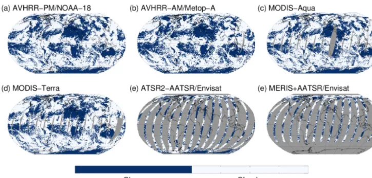
Measurements from the passive imaging sensors AVHRR, MODIS, ATSR2, AATSR and MERIS sensors were used to produce the Cloud_cci datasets. Each sensor has different imaging characteristics, such as differences in swath width, which leads to varying observation frequency for any given position on Earth. All sensors operate in a sun-synchronous polar orbit. Each individual orbit has an ascending and de-scending part, which roughly corresponds to either daytime or night-time conditions, which are thus also referred to as daytime and night-time node. For the MERIS+AATSR dataset, the night-time observations are ignored. Individual AVHRR and MODIS sensors cover the globe nearly twice a day with the daytime and night-time nodes of their orbits. Due to their narrow swath width, ATSR2 and AATSR need 3 days to cover the full globe with daytime and night-time ob-servations (Fig. 2). With respect to the local Equator-crossing time of the daytime node, the AVHRR-carrying satellites were separated into AM (a.m. – ante meridiem, before noon) and PM (p.m. – post meridiem, after noon). In the following sections further characteristics of the measurement data that form the basis of the Cloud_cci datasets are summarized.
2.1.1 AVHRR
Figure 1.Overview of all sensors processed in Cloud_cci and their duration as a function of the daytime Equator-crossing time (AM: ante meridiem, before noon; PM: post meridiem, after noon). Sensors belonging to the same dataset are shown in the same colour.
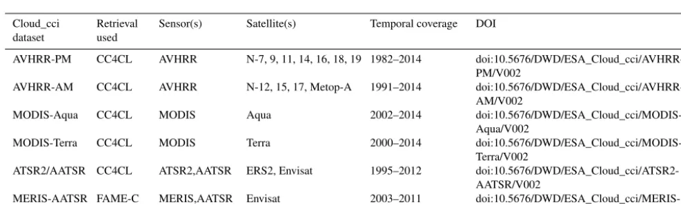
Table 1.List of Cloud_cci datasets together with the corresponding retrieval scheme, the sensor(s), satellite(s) used and the time period covered as well as the digital object identifiers (DOIs) issued.
Cloud_cci dataset
Retrieval used
Sensor(s) Satellite(s) Temporal coverage DOI
AVHRR-PM CC4CL AVHRR N-7, 9, 11, 14, 16, 18, 19 1982–2014 doi:10.5676/DWD/ESA_Cloud_cci/AVHRR-PM/V002
AVHRR-AM CC4CL AVHRR N-12, 15, 17, Metop-A 1991–2014 doi:10.5676/DWD/ESA_Cloud_cci/AVHRR-AM/V002
MODIS-Aqua CC4CL MODIS Aqua 2002–2014
doi:10.5676/DWD/ESA_Cloud_cci/MODIS-Aqua/V002
MODIS-Terra CC4CL MODIS Terra 2000–2014
doi:10.5676/DWD/ESA_Cloud_cci/MODIS-Terra/V002
ATSR2/AATSR CC4CL ATSR2,AATSR ERS2, Envisat 1995–2012 doi:10.5676/DWD/ESA_Cloud_cci/ATSR2-AATSR/V002
MERIS-AATSR FAME-C MERIS,AATSR Envisat 2003–2011
doi:10.5676/DWD/ESA_Cloud_cci/MERIS-AATSR/V002
AM: ante meridiem, before noon; PM: post meridiem, after noon; CC4CL: Community Cloud retrieval for CLimate; FAME-C: Freie Universität Berlin AATSR MERIS Cloud retrieval; N: NOAA.
width is 2399 km, which facilitates full global cover-age (daytime and night-time) twice daily. More infor-mation about the AVHRR sensor can for example be found at https://www.wmo-sat.info/oscar/instruments/view/ 62. The Cloud_cci AVHRR-AM and AVHRR-PM datasets are based on measurements from AVHRR/2 and AVHRR/3 on board prime polar-orbiting NOAA POES and Metop satellites, i.e. AVHRR-PM: NOAA-7, NOAA-9, NOAA-11, NOAA-14, NOAA-16, NOAA-18 and NOAA-19; AVHRR-AM: NOAA-12, NOAA-15, NOAA-17 and Metop-A. All measurements used are global area coverage (GAC) data with a footprint size of 1.1 km×4.4 km and a sampling dis-tance of 3.3 km along track and 5.5 km across track between the centres of the GAC footprints. GAC data are derived from the originally measured Local Area Coverage (LAC, foot-print size: 1.1 km×1.1 km) data by on-board averaging of four neighbouring LAC pixels every third scan line. Only the GAC record is available for AVHRR with global and nearly seamless temporal coverage since the early NOAA satellites.
The two visible channels and the 1.6 µm channel (if present) were intercalibrated using MODIS Collection 6 measure-ments (Heidinger et al., 2017; an update of Heidinger et al., 2010). For the IR channels no further calibration was per-formed beyond the on-board blackbody calibration.
2.1.2 MODIS
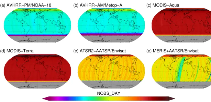
Level-Figure 2.Daily Level-3U cloud mask composites for 22 June 2008 demonstrating the spatial coverage of the daytime nodes of selected sensors within 24 h. See Table 3 for definition of Level-3U.
1b data of the Collection 6 release were obtained from NASA. The Collection 6 Level-1 data are expected to show several improvements over Collection 5 data due to im-proved calibration methodologies (see for example http:// mcst.gsfc.nasa.gov/calibration/collection_6_info). The foot-print size of the MODIS Level-1 data is 0.25 km×0.25 km to 1 km×1 km (depending on channel); here we used data at 1 km×1 km resolution for all channels.
2.1.3 ATSR2 and AATSR
The passive imaging sensors ATSR2 and AATSR have seven spectral channels in the solar, near-infrared and ther-mal infrared range with central wavelengths between 0.55 and 12 µm, of which five (the AVHRR heritage channels; ATSR2/AATSR channel numbers 2, 3, 5, 6, 7) were used. At nadir the ATSR2 and AATSR pixel resolution is ap-proximately 1 km×1 km with a swath width of 500 km. The sensor is designed to be self-calibrating. Two integrated thermally controlled blackbody targets are used for cali-bration of the thermal channels, while an opal visible cal-ibration target illuminated by sunlight is used for calibra-tion of visible and near-infrared channels. More informacalibra-tion about the ATSR-2 and AATSR sensors is available at https: //www.wmo-sat.info/oscar/instruments/view/56 and https:// www.wmo-sat.info/oscar/instruments/view/2. Version 3.1 of the ATSR2 and AATSR Level-1 data was used. The available ATSR2 Level-1 record covers 1995–2002, while the AATSR Level-1 record covers 2002–2012.
2.1.4 MERIS
MERIS is a passive imaging sensor whose measurements were synergistically combined with AATSR measurements in this study, making use of the fact that both sensors are
mounted on the same platform (Envisat) but have comple-mentary spectral characteristics. The pixels of both sensors were spatially matched. MERIS measurements outside the AATSR swath width (500 km, which is narrower than the MERIS swath width of 1150 km) were not used. The collocated synergy product has a swath width of 493 pixels. This is related to collocating the curved AATSR grid with the MERIS grid. More information on the matching procedure can be found in (Gómez-Chova et al., 2009). The spatial resolution of the MERIS reduced resolution mode is 1.2 km×1 km and thus very similar to AATSR. More infor-mation about the MERIS sensor is available at https://www. wmo-sat.info/oscar/instruments/view/277. MERIS Level-1 data of the third reprocessing has been used (https://earth. esa.int/documents/700255/707222/A879-NT-017-ACR_ v1.0.pdf/6fa86bec-9945-4e39-808e-3801f2e3962b). In addition to the above-mentioned AVHRR heritage channels of AATSR, MERIS channel 11 (spectrally located in the oxygen-A absorption band around 761 nm) and channel 10 (a nearby window channel located around 753 nm) were used. An empirical stray-light correction was applied to the reflectance of the MERIS oxygen-A absorption band channel (Lindstrot et al., 2010). For this correction, the spectral smile effect in the MERIS measurements (Bourg et al., 2008), which is the variation in the channel centre wavelength along the field of view, as well as the amount of stray light in the MERIS oxygen-A absorption band channel, was determined.
2.2 Retrieval systems
the Cloud_cci climate records. For datasets derived from AVHRR and from the AVHRR heritage channels of MODIS, ATSR-2 and AATSR, the Community Cloud retrieval for CLimate (CC4CL; Sus et al., 2017; McGarragh et al., 2017b) retrieval system was employed. For the MERIS+AATSR dataset, the Freie Universität Berlin AATSR MERIS Cloud (FAME-C; Carbajal Henken et al., 2014) retrieval sys-tem was employed. Common to both syssys-tems is the OE technique, which uses a Levenberg–Marquardt (Levenberg, 1944; Marquardt, 1963; Rodgers, 2000) non-linear inversion method to iteratively fit simulated TOA radiances to the mea-sured TOA radiances. The ability to include a prior knowl-edge of the retrieved quantities is built into the method. The OE technique supports comprehensive error propagation, al-lowing measurement error, forward model error (due to ap-proximations and assumptions, which are made in the mod-elling of TOA radiance) and uncertainties in a priori knowl-edge to be combined to give a rigorous estimate of the uncer-tainty on retrieved values on a pixel-by-pixel basis.
CC4CL and FAME-C were employed to primarily retrieve the following cloud properties: cloud mask (CMA), cloud phase (CPH), cloud optical thickness (COT), cloud effec-tive radius (CER) and cloud-top pressure (CTP). From these properties, cloud-top temperature (CTT), cloud-top height (CTH), liquid water path (LWP), ice water path (IWP) and cloud albedo (CLA) were also determined. A short descrip-tion of all cloud properties is given in Table 2. The next two subsections briefly summarize the main characteristics of CC4CL and FAME-C with in-depth details to be found in the references given therein.
2.2.1 CC4CL
The CC4CL retrieval system has three main components: cloud detection to retrieve CMA; cloud typing to retrieve CPH; and an OE retrieval of COT, CER and CTP. The three components are framed by a pre-processing (e.g. spatio-temporal mapping of all data fields and clear-sky radiative transfer simulations) and a post-processing (e.g. merging, consistency check, quality control). The cloud detection is performed by applying an artificial neural network (ANN) that uses the AVHRR heritage channel measurements, illu-mination, scan angles, and auxiliary data as input. The ANN was trained to mimic the COT of the Cloud-Aerosol Li-dar with Orthogonal Polarization (CALIOP; Winker et al., 2009), which is the main payload of the Cloud-Aerosol Lidar and Infrared Pathfinder Satellite Observations (CALIPSO) satellite. Cloudy pixels are identified where the ANN-estimated COT exceeds pdefined thresholds (with the re-maining pixels classified as clear), thus defining the CMA. Based on CALIOP data in the ANN training set, a cloud mask uncertainty is determined. The cloud typing is based on a threshold decision tree documented in (Pavolonis and Heidinger, 2004) and (Pavolonis et al., 2005). Various cloud types exist for either liquid or ice phase, which allows the
simplification to a binary CPH information. The central part of CC4CL is an OE estimation of COT, CER and CTP, which is based on earlier developments of the Oxford RAL retrieval of Aerosol and Cloud retrieval (ORAC; Poulsen et al., 2012; Watts et al., 1998) but has undergone major updates since then. As mentioned above, a cloud model is iteratively mod-ified to fit the simulated radiances to the measurements. For this, a fast forward radiative transfer model is included us-ing scalar reflectance, transmission and emission operators. These operators interact with (1) the direct beam solar source and/or the diffuse thermal source from above and (2) both direct and diffuse surface reflectance from a bidirectional re-flectance distribution function (BRDF) surface in the solar channels, as well as diffuse atmospheric and surface emission in the thermal channels from below. The operators are a func-tion of the state vector elements COT and CER, and solar and instrument geometry and compiled in look-up tables (LUTs) precalculated using the DIScrete Ordinates Radiative Trans-fer (DISORT; Stamnes et al., 1988) solver. The simulations were done separately for liquid and ice clouds. Liquid clouds are represented with a modified gamma distribution (Hansen and Travis, 1974) and ice cloud single-scattering properties are taken from (Baran et al., 2005).
Clear-sky transmittance and radiance profiles are com-puted using the Radiative Transfer for Television Infrared Observation Satellite Program (TIROS) Operational Verti-cal Sounder (TOVS) (RTTOV; Eyre, 1991; Saunders et al., 1999) model version 11.3 (Hocking et al., 2014). For each it-eration the above-cloud and below-cloud clear-sky transmit-tances and radiances are interpolated from the correspond-ing RTTOV profiles as a function of CTP. From the derived state vector variables, the properties CTT, CTH, CLA, LWP and IWP are inferred with LWP and IWP calculations being based on (Stephens, 1978) for all cloudy conditions. A full list of retrieved cloud variables is given in Table 2. The reader is referred to (Sus et al., 2017) and (McGarragh et al., 2017b) for more details on CC4CL. The CC4CL system was used for the generation of the Cloud_cci datasets AVHRR-PM, AVHRR-AM, MODIS-Aqua, MODIS-Terra and ATSR2-AATSR.
2.2.2 FAME-C
re-flectances were composed through radiative transfer simu-lations utilizing the Matrix Operator Model (MOMO; Fis-cher and Grassl, 1984; Fell and FisFis-cher, 2001). From the retrieved COT and CER, LWP and IWP are computed us-ing (Stephens, 1978) for liquid clouds and optically thick ice clouds. For optically thin ice clouds, the conversion of (Heymsfield et al., 2003) is applied. Using the retrieved CPH and COT, a cloud-top temperature retrieval is conducted us-ing the AATSR thermal infrared channels. Radiative transfer simulations for AATSR are done using RTTOV version 11.2. The CTT is further converted to CTH and CTP using collo-cated numerical weather prediction (NWP) profiles of pres-sure, temperature and height. These CTP values are provided as first guess to a second CTP retrieval based on MERIS measurements in an oxygen-A absorption band channel and a nearby window channel. The difference in sensitivity of both cloud height retrievals to different kinds of cloudy situations was analysed in (Carbajal Henken et al., 2015).
The full list of retrieved cloud properties using the FAME-C system largely overlaps with the FAME-CFAME-C4FAME-CL output and is thus also given in Table 2. The reader is referred to (Car-bajal Henken et al., 2014) for more details on the FAME-C. The FAME-C system was used for the generation of the Cloud_cci MERIS+AATSR dataset.
2.3 Product definitions
The full suite of Level-2 cloud properties derived from both retrieval systems is CMA, CPH, CTP, CTH, CTT, COT, CER, CWP, and CLA (at two wavelengths), where CWP represents either LWP in pixels with liquid clouds or IWP in pixels with ice clouds. Nearly all of these properties are accompanied by uncertainty measures that are direct outputs of OE (or derived from them). Exceptions are CC4CL CMA, for which the un-certainty is empirically estimated from validation work (Sus et al., 2017). Furthermore, CMA from FAME-C and CPH from both retrieval systems are not accompanied by uncer-tainty information yet. Besides Level-2, two additional pro-cessing levels exist: Level-3U and Level-3C, which are ex-plained in Sect. 2.4.
2.4 From pixel-based retrieval data (Level-2) to daily and monthly properties (Level-3)
Level-2 data were the input to the Level-3 processing and underwent a spatio-temporal sampling and averaging. Level-3U products are global composites, defined on a latitude– longitude grid at 0.05◦×0.05◦ resolution. Level-3U fields
hold Level-2 data which were sampled into the Level-3U grid within a 24 h time window. The most important aspects of this sampling procedure are as follows: (1) only that Level-2 pixel that has the lowest satellite zenith angle is kept in each Level-3U grid cell and (2) the actual footprint size of each pixel is considered (which depends on the sensor and scan angle), which can lead to more than one Level-3U grid
cell being filled by one single Level-2 pixel observations. The Level-3U composition was done for each day, keeping the ascending and descending nodes of the orbits in separate fields, which roughly corresponds to separating daytime and night-time observations. The Level-3U products also hold a variety of ancillary data information apart from the retrieved cloud properties. Taking advantage of the high spatial reso-lution of the MODIS sensor, additional Level-3U products were produced for MODIS for a 0.02◦×0.02◦grid covering the European area within 15◦W to 45◦E and 35 to 75◦N (not shown).
Level-3C products are defined on a latitude–longitude grid with 0.5◦×0.5◦ resolution and hold monthly summaries of the Level-2 data, such as averages and standard deviation. In addition, monthly histograms were composed for CTP, CTT, CER, COT, CWP, CLA, each separated into liquid and ice clouds, and for combinations of COT and CTP (joint cloud property histogram, JCH). Table 3 summarizes most impor-tant characteristics of all processing levels. The binning of the Level-3C histograms is given in Table 5. Table 4 reflects the available cloud properties for each processing level.
Due to differences in spatial resolution and swath width between the considered sensors, the spatio-temporal observa-tion frequency is very different. The effect of this on monthly scale is demonstrated in Fig. 3 by the number of daytime ob-servations per 0.5◦grid cell per month.
2.4.1 Propagating the uncertainties
Different metrics can be used to represent the uncertainty of monthly mean Level-3C products. A simple and often used metric is the standard deviationσSD(Eq. 1) calculated over the same set of retrieved pixels (xi) that is used for the calcu-lation of the mean (hxi):
σSD2 = 1 N
N
X
i=1
(xi− hxi)2, (1)
withNbeing the number of pixels.
The OE approach provides pixel-based retrieval uncertain-ties (σi) that are based on mathematically consistent propa-gation of the uncertainties of the input data (e.g. auxiliary data, measurement data, background errors) into the Level-2 product space (see for example McGarragh et al., Level-2017b, and Sus et al., 2017). For the Cloud_cci datasets, the Level-2 uncertainties were further propagated into Level-3C products by two measures: the mean of the pixel-based uncertainties (hσii, Eq. 2) and the mean of the squares of the pixel-based uncertainties (hσi2i, Eq. 3).
hσii = 1
N N
X
i=1
(σi) (2)
hσi2i = 1 N
N
X
i=1
Table 2.List of generated cloud properties. See Sect. 2.4 for more information on the processing levels Level-2, Level-3U and Level-3C.
Variable Abbreviation Definition
Cloud mask
Cloud fractional cover
CMA CFC
A binary cloud mask per pixel (Level-2, Level-3U)
Subsequently calculated monthly total cloud fractional cover (Level-3C); also separated into three vertical classes (high, mid-level, low clouds) following ISCCP classification of (Rossow and Schiffer, 1999).
Cloud phase Liquid cloud fraction
CPH The thermodynamic phase of the cloud (binary: liquid or ice; in Level-2, Level-3U) The monthly liquid cloud fraction (Level-3C) using the binary cloud phase information.
Cloud optical thickness COT The line integral of the absorption and the scattering coefficients along the vertical in cloudy pixels.
Cloud effective radius CER The projected-area-weighted mean radius of the cloud drop and crystal particles, re-spectively.
Cloud-top pressure Cloud-top height Cloud-top temperature
CTP CTH CTT
The air pressure at the top of the uppermost cloud layer – direct output of OE. Height of cloud top, inferred from CTP using ERA-Interim (Dee et al., 2011) profiles. Air temperature at the cloud top, inferred from CTP using ERA-Interim profiles.
Cloud water path (containing ice and liquid water path)
CWP (LWP, IWP)
The vertically integrated liquid/ice water content in a cloudy column; derived from CER and COT following (Stephens, 1978).
Joint cloud property histogram JCH A spatially resolved two-dimensional histogram of combinations of COT and CTP for each spatial grid cell (Level-3C only).
Spectral cloud albedo at 0.6 µm Spectral cloud albedo at 0.8 µm
CLA_vis006 CLA_vis008*
The black-sky albedo derived for channel 1 (0.67 µm) and 2 (0.87 µm∗), respectively (experimental product).
∗
For FAME-C, the cloud albedo is derived at 1.6 µm instead of 0.87 µm.
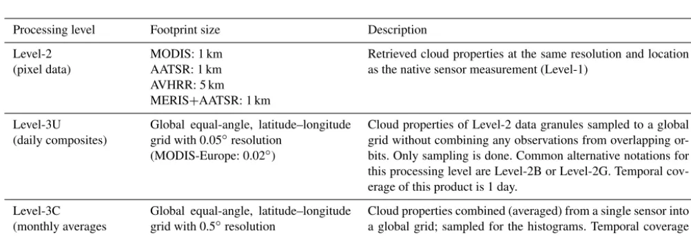
Table 3.Processing levels of Cloud_cci data products. The footprint refers to the area on the Earth’s surface that is covered by one sensor pixel at nadir view.
Processing level Footprint size Description
Level-2 (pixel data)
MODIS: 1 km AATSR: 1 km AVHRR: 5 km MERIS+AATSR: 1 km
Retrieved cloud properties at the same resolution and location as the native sensor measurement (Level-1)
Level-3U (daily composites)
Global equal-angle, latitude–longitude grid with 0.05◦resolution
(MODIS-Europe: 0.02◦)
Cloud properties of Level-2 data granules sampled to a global grid without combining any observations from overlapping or-bits. Only sampling is done. Common alternative notations for this processing level are Level-2B or Level-2G. Temporal cov-erage of this product is 1 day.
Level-3C (monthly averages and histograms)
Global equal-angle, latitude–longitude grid with 0.5◦resolution
Cloud properties combined (averaged) from a single sensor into a global grid; sampled for the histograms. Temporal coverage of this product is 1 month.
With these measures it is possible to include the OE-based Level-2 uncertainties when quantifying both the true, natural variability (σtrue) of the observed geophysical variable (Eq. 4) and the uncertainty of the calculated mean (σhxi, Eq. 5).
σtrue2 =σSD2 −(1−c)hσi2i (4)
σh2xi=
1
Nσ 2
true+chσii2+(1−c) 1
Nhσ 2
i i (5)
These equations assume a bias-free Gaussian distribution for both the Level-2 uncertainties and the retrieved variables. This assumption is inaccurate for many variables of the
pre-sented properties, which introduces some limitations to the presented approach. Hence, the propagated uncertainties are meant to be experimental for these dataset versions. Assum-ing Gaussian and bias-free distributions, the estimated natu-ral variability represents the standard deviation (thus the in-ner 68 % percentile) of the distribution around the true mean. Furthermore, the estimated uncertainty of the monthly mean represents the 68 % confidence interval around the calculated monthly mean.
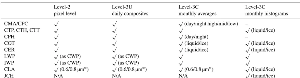
Table 4.Cloud_cci product portfolio, also featuring day/night and liquid/ice separation for some properties. All products listed exist for each dataset.
Level-2 pixel level
Level-3U daily composites
Level-3C monthly averages
Level-3C
monthly histograms
CMA/CFC √ √ √(day/night high/mid/low) –
CTP, CTH, CTT √ √ √ √(liquid/ice)
CPH √ √ √(day/night) –
COT √ √ √(liquid/ice) √(liquid/ice)
CER √ √ √(liquid/ice) √(liquid/ice)
LWP √(as CWP) √(as CWP) √ √
IWP √(as CWP) √(as CWP) √ √
CLA √(0.6/0.8 µm∗) √(0.6/0.8 µm∗) √(0.6/0.8 µm∗) √(liquid/ice)
JCH N/A N/A N/A √(liquid/ice)
∗For FAME-C, the cloud albedo is derived at 1.6 µm instead of 0.87 µm.
Table 5.Bin borders of Cloud_cci Level-3C histograms of cloud-top pressure (CTP), cloud-top temperature (CTT), cloud optical thickness (COT), cloud effective radius (CER), liquid and ice water path (CWP), cloud albedo (CLA), and joint cloud property histogram (JCH).
Cloud_cci variable Bin borders in Level-3C monthly histograms
CTP (hPa) 1, 90, 180, 245, 310, 375, 440, 500, 560, 620, 680, 740, 800, 875, 950, 1100 CTT (K) 200, 210, 220, 230, 235, 240, 245, 250, 255, 260, 265, 270, 280, 290, 300, 310, 350 COT 0, 0.3, 0.6, 1.3, 2.2, 3.6, 5.8, 9.4, 15, 23, 41, 60, 80, 99.99, 1000
CER (µm) 0, 3, 6, 9, 12, 15, 20, 25, 30, 40, 60, 80
CWP (g m−2) 0, 5, 10, 20, 35, 50, 75, 100, 150, 200, 300, 500, 1000, 2000, 100 000 CLA_vis006/008∗ 0, 0.1, 0.2, 0.3, 0.4, 0.5, 0.55, 0.6, 0.65, 0.7, 0.75, 0.8, 0.9, 1 JCH See COT and CTP bins
∗For FAME-C, the cloud albedo is derived at 1.6 µm instead of 0.87 µm.
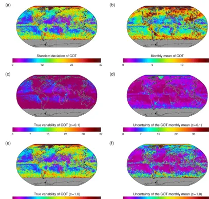
Level-3C products. The results are discussed using the ex-ample of COT from the AVHRR-PM dataset for June 2008. Figure 4 shows global maps of monthly mean COT and the corresponding monthly standard deviation (panels a and b) as calculated from the retrieved Level-2 values. The estimate of the true variability is shown along with the estimated certainty of the calculated mean (panels c and d) for an un-certainty correlation (c) of 0.1. Panels (e) and (f) show the results for an uncertainty correlation of 1.0. The exact corre-lation is not known and it is likely to have spatial and tem-poral variability. Due to this, two very different values have been chosen to illustrate the sensitivity. In this example, re-gions with high mean COT tend to be characterized by high spatio-temporal variability in the underlying data, which is apparent in the increased standard deviation. An exception is the northern part of the Atlantic and Pacific oceans, where the standard deviation is low while the mean COT is high. A noticeable feature is found in the stratocumulus regions, which are located in the eastern parts of the subtropical ocean regions. There, the COT is very stable and thus shows low standard deviations. Another very dominant feature is a band of rather high mean COT accompanied with high variability, in the storm track regions of the Southern Ocean.
Now, assuming a rather low uncertainty correlation of 0.1, the estimated true variability becomes very small (Fig. 4c).
This is due to the second term on the right side of Eq. (4), in which the mean of the squared retrieval uncertainties is not significantly reduced when using a correlation of 0.1. In other words, if the retrieval uncertainties are only slightly correlated, they contribute to a broadening of the observed COT distribution, causing only a minor systematic shift of the distribution. In this scenario, the retrieval uncertainties can explain a large portion of the observed standard devi-ation. In some regions the second term of Eq. (4) is even larger than the first term (the observed variance), which re-sults in negative values of the estimated natural variability. Such negative values are non-physical and indicate an im-proper correlation in corresponding regions. They have been set to 0 in the plots. The uncertainty of the mean is also rel-atively small for a correlation of 0.1 (Fig. 4d). This is due to all three terms of Eq. (5) becoming small: the third term because of the relatively largeN, the second term because of the low correlation and the first term because of the low estimated natural variability, additionally minimized by the division byN. In other words, having small systematic un-certainties (i.e. a low uncertainty correlation) leads to a low uncertainty of the mean, which is dominated by sampling un-certainties decreasing with increasingN.
Figure 3.Number of daytime observations (pixels) per 0.5◦grid cell for June 2008 and(a)AVHRR-PM/NOAA-18,(b) AVHRR-AM/Metop-A,(c)MODIS-Aqua,(d)MODIS-Terra,(e)AATSR and(f)MERIS+AATSR. For the sake of comparability only the daytime number is shown because no night-time observations are included in MERIS+AATSR. Grey-shaded areas indicate regions with no daylight and thus without daytime observations.
the right hand side of Eq. (4) vanishes in this case, leading to the estimated true variability being equal to the observed standard deviation. The uncertainty of the mean is also in-creased, which is in contrast to the previous scenario with low correlation. A correlation of 1.0 eliminates the third term of Eq. (5). The first term decreases with larger N, although the natural variability is now larger than the previous exam-ple, leaving the second term dominating the uncertainty on the mean, which is the arithmetical mean of the retrieval certainties. Since for cloud optical thickness the retrieval un-certainty is usually highest for clouds with high COTs, the uncertainty of the mean is highest in regions dominated by such clouds.
The Cloud_cci Level-3C products contain the individual uncertainty termsσSD,hσiiandhσi2ifor each variable in ad-dition to the mean. This allows posterior calculations ofσhxi
andσtruefor any given uncertainty correlation.
3 Product examples
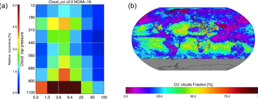
In this section most Cloud_cci products are discussed using the example of the AVHRR-PM dataset, i.e. (1) Level-3U data of NOAA-18/AVHRR for 22 June 2008 and (2) Level-3C data for the month of June 2008. Figure 5 shows CMA, CFC, CPH, liquid cloud fraction, COT and CER. Figure 6 shows CTP, LWP, IWP and CLA. In Fig. 7 the JCH is pre-sented in two ways: (1) shown as a global COT-CTP his-togram aggregated over all grid cells and (2) the relative fraction of a certain subset of clouds, in this case cumulus clouds according to the ISCCP definition given in (Rossow and Schiffer, 1999): clouds with CTP larger than 680 hPa and with COT lower than 3.6.
Figure 4.Monthly standard deviation(a)and monthly mean(b)for cloud optical thickness (COT). Panels(c)and(d)show the estimated natural variability and uncertainty of the mean(d)for a correlation of 0.1. Panels(e)and(f)are the same as panels(c)and(d)but for an uncertainty correlation of 1.0. All data are from AVHRR-PM in June 2008.
and should be applied precedent to any trend analysis. The impact of spectral deviation among the individual AVHRR sensors of a dataset is assumed to have a smaller impact com-pared to the satellite drift effect. For ATSR2-AATSR a small jump in the time series of some cloud properties is found at the sensor transition. This is primarily driven by differences in the dynamic range of the 3.7 µm channel. The channel sat-urates more often for ATSR-2. This is particularly evident for CFC, LWP and IWP.
Another feature in the AVHRR-PM CFC time series (Fig. 9) is worth mentioning. In 1982 (and onwards) and in 1991 (and onwards) positive anomalies are found which are related to the major eruptions of the El Chichón (Mex-ico) and Pinatubo (Philippines) volcanoes. A first analysis revealed that heavy aerosol loadings are sometimes detected as clouds. As this seems to be a general feature of CC4CL and FAME-C, cloud detection and cloud-top properties of all
datasets should be used with caution in heavy aerosol condi-tions.
4 Validation summary
Figure 5.Level-3U(a, c, e, g)and Level-3C(b, d, f, h) of cloud mask/fraction(a–b), cloud phase/liquid cloud fraction(c–d), optical thickness(e–f)and effective radius(g–h)for the AVHRR-PM dataset for June 2008. For the Level-3U examples, the ascending nodes of the orbits are shown, which roughly correspond to the daylight portions of the orbits of NOAA-18. COT, LWP, IWP and CLA are only retrieved during daytime conditions. Areas with no valid retrievals in this day/month are grey-shaded.
is expected that Cloud_cci CTHs are lower than those ob-served by CALIOP, in particular for clouds containing fuzzy (semi-transparent) cloud layers. To account for this, various metrics have been considered for the validation of Cloud_cci cloud properties, where the CALIOP properties have been adjusted with respect to the optical depth profile.
The CAL_LID_L2_05kmCLay-Prov product has been used, which was downloaded from ICARE Data and Ser-vice Center (http://www.icare.univ-lille1.fr). All collocations
ATSR2-Figure 6.As Fig. 5 but for cloud-top pressure(a–b), liquid water path(c–d), ice water path(e–f), and spectral cloud albedo at 0.6 µm(g–h)
for Level-3U(a, c, e, g)and Level-3C(b, d, f, h)products. Panels(c)and(e)both show the Level-3U cloud water path, which represents liquid water path in liquid cloud pixels and ice water path in ice cloud pixels.
AATSR and MERIS+AATSR datasets) and Terra deviate significantly from CALIPSO. Thus, for these satellites the collocation time window was extended to ±15 min. These collocations are, however, still limited to the very high lati-tudes around 70◦north and south and are thus occasionally affected by snow and ice as well as low solar-zenith-angle conditions.
In Table 6 the validation results for CMA are presented, i.e. the probabilities of correctly detecting cloudy and clear-sky scenes (Hit rate, PODcloudy, PODclear; see Appendix A
Figure 7.(a)Joint cloud property histogram, globally aggregated over all grid cells.(b)Global map of relative occurrence of cumulus clouds (according to ISCCP definition of Rossow and Schiffer, 1999 with CTP>680 hPa and COT<3.6) with respect to all clouds. Data shown are from AVHRR-PM in June 2008.
Table 6.Summary of cloud mask (CMA) validation results for Cloud_cci datasets when compared against CALIOP. Validation measures are the probabilities of detecting cloudy and clear scenes (Hit rate, PODliquid, PODice; see Appendix A for the definition of these terms) and bias. Also given is the number of collocated pixels. The scores are separated into two cloud optical thickness thresholds (COTthres) representing above which CALIOP COT the CALIOP pixel was classified cloudy.
Score AVHRR-AM AVHRR-PM MODIS-Terra∗ MODIS-Aqua ATSR2-AATSR∗ MERIS+AATSR∗
COD
le
v
=
0
.
0 Hit rate (%) 76.2 81.2 91.0 81.6 74.3 73.4
PODcloudy(%) 78.3 79.0 94.4 81.1 80.0 74.6
PODclear(%) 70.4 87.7 70.0 83.1 60.5 69.6
Bias (%) −8.1 −12.6 −1.1 −9.8 −2.6 −12.5
Number 42 119 16 675 575 19 118 16 494 437 94 039 23 098
COD
le
v
=
0
.
15 Hit rate (%) 78.3 84.9 89.4 83.5 75.0 75.6
PODcloudy(%) 84.4 87.5 96.5 88.7 86.2 80.3
PODclear(%) 67.6 80.5 51.7 75.0 58.4 66.4
Bias (%) 1.9 −0.5 4.8 2.3 8.5 −1.5
Number 42 119 16 675 575 19 118 16 494 437 94 039 23 098
∗Time window used for collocations was±15 min for ATSR2+AATSR, MERIS+AATSR and MODIS-Terra. For all others a±3 min window was used.
datasets, which can be explained by the higher frequency of cloudy scenes compared to clear-sky scenes. Removing opti-cally very thin clouds from the CALIOP data (i.e. classifying all clouds with optical thickness lower than 0.15 as clear sky in the CALIOP data) significantly improves the agreement of Cloud_cci data with CALIOP (lower part of Table 6). The hit rates are mostly increased (except for MODIS-Terra) and the biases are reduced (except MODIS-Terra and ATSR2-AATSR).
In Table 7 the validation results for CPH are presented, i.e. the probabilities of correctly detecting liquid and ice clouds (Hit rate, PODliquid, PODice; see Appendix A for the defi-nition of these terms), the bias and the number of consid-ered cloudy pixels. As for CMA, two validation set-ups have been used: in the first the CALIOP cloud phase from the uppermost reported cloud layer was used (upper part of
Ta-ble 7), while in the second set-up the CALIOP cloud phase was taken at that level in the cloud at which the top-down cloud optical depth is 0.15 or higher (CODlev=0.15; lower part of Table 7). For the first set-up, the probabilities of de-tecting the correct phase range from 72 to 78 %, with high-est values for AVHRR-PM and ATSR2-AATSR. All datasets
except MERIS+AATSR and ATSR2-AATSR show a clear
Figure 8.Time series of monthly mean cloud properties of Cloud_cci datasets, with thin lines being (from top to bottom) time series of monthly mean cloud fraction (CFC), liquid cloud fraction (CPH), cloud-top pressure (CTP), cloud optical thickness (COT), cloud effective radius (CER), liquid water path (LWP) and ice water path (IWP), overlaid with a running average (thick lines). Shown are those Cloud_cci datasets that are based on so-called morning satellites. The monthly means are calculated for 60◦S–60◦N (latitude-weighted). The time series shown have not been corrected for satellite drift or diurnal cycle.
the detection efficiency for liquid phase (PODliq) decreases only slightly. The biases change towards ice (reduced liquid bias or ice bias instead of liquid bias). The results show that the correct cloud phase determination for passive imager re-trieval is very sensitive to phase changes in the uppermost cloud layers (e.g. between the physical cloud top and 1 op-tical depth into the cloud). In addition to the CPH compar-isons presented, the scores were again calculated including only conditions for which no phase change occurred in the CALIOP data between the physical cloud top and 1 optical depth into the cloud (not shown). The agreement between
Cloud_cci datasets and CALIOP data further improves sig-nificantly. Hit rates increase by 2 to 10 %, mainly driven by a much better detection probability for ice clouds.
Figure 9.As Fig. 8 but for Cloud_cci datasets based on afternoon satellites. The time series shown have not been corrected for satellite drift or diurnal cycle.
picture of the actual cloud-top height retrieval, since the first guess of COT, CER and CTP in the Cloud_cci retrieval sys-tems is a function of the prior determined cloud phase. The comparisons were separated into liquid and ice cloud con-ditions and carried out twice using different top-down cloud optical depth levels (CODlev) at which the reference CTH was selected from CALIOP profiles. For liquid clouds the standard deviation between Cloud_cci datasets and CALIOP is around 1 km and the bias is generally below 0.2 km (ex-cept MERIS+AATSR with a bias of 0.79 km). These val-ues do not change significantly when selecting the refer-ence CALIOP CTH at CODlev=0.15 (bottom part of Ta-ble 8), which indicates that water clouds usually do not have small optical thicknesses. For ice clouds the agreement with
Table 7.Summary of cloud phase (CPH) validation results for Cloud_cci datasets when compared against CALIOP. Validation measures are probability of detection (POD) and bias of liquid cloud occurrence. Also given is the number of collocated pixels. The scores are separated into two cloud optical depth levels (CODlev) representing at which top-down COD into the cloud the reference CALIOP CPH was taken.
Score AVHRR-AM AVHRR-PM MODIS-Terra∗ MODIS-Aqua ATSR2-AATSR∗ MERIS+AATSR∗
COD
le
v
=
0
.
0 Hit rate (%) 72.0 77.1 74.4 73.7 77.6 72.3
PODliq(%) 71.3 78.0 88.1 82.7 67.7 67.3
PODice(%) 72.5 76.5 65.1 68.1 83.1 76.9
Bias (%) 6.4 5.9 15.9 13.0 −0.6 −3.5
Number 23 151 9 436 914 15 581 9 576 169 50 659 9210
COD
le
v
=
0
.
15 Hit rate (%) 76.0 80.6 80.7 79.6 77.8 73.8
PODliq(%) 70.8 74.0 85.7 79.6 64.6 64.2
PODice(%) 81.2 87.4 74.6 79.6 89.7 88.6
Bias (%) −5.1 −6.9 5.0 −0.27 −11.3 −17.3
Number 22 221 8 935 688 15 213 8 951 056 47 527 8770
∗Time window used for collocations was±15 min for ATSR2+AATSR, MERIS+AATSR and MODIS-Terra. For all others a±3 min window was used.
Table 8.Summary of cloud-top height (CTH) validation results for Cloud_cci datasets when compared against CALIOP. Validation measures are standard deviation (SD) and bias. Also given is the number of collocated pixels. All scores are separated into liquid and ice clouds (both Cloud_cci dataset and CALIOP had to agree on phase) and into two cloud optical depth levels (CODlev) representing at which top-down COD into the cloud the reference CALIOP CTH was taken.
Score AVHRR-AM AVHRR-PM MODIS-Terra∗ MODIS-Aqua ATSR2-AATSR∗ MERIS+AATSR∗
COD
le
v
=
0
.
0 SD
liq(km) 1.04 0.91 0.75 0.97 0.89 1.35
Biasliq(km) 0.17 −0.12 0.04 −0.09 0.11 0.79
Numberliq 6177 2 850 732 5552 4 041 688 12 149 2836
SDice(km) 2.66 2.84 1.91 2.79 2.33 1.90
Biasice(km) −2.66 −2.65 −2.65 −2.57 −2.59 −3.59
Numberice 10 468 4 417 179 6041 4 014 001 27 164 3614
COD
le
v
=
0
.
15 SDliq(km) 1.06 0.97 0.85 1.03 0.94 1.35
Biasliq(km) 0.14 −0.09 0.08 −0.06 0.13 0.82
Numberliq 7807 3 335 953 6688 3 596 738 14 508 3300
SDice(km) 2.56 2.59 1.73 2.51 2.04 1.79
Biasice(km) −1.96 −1.94 −2.21 −1.90 −1.95 −2.82
Numberice 9046 3 865 027 5521 3 524 716 22 455 3001
∗Time window used for collocations was±15 min for ATSR2+AATSR, MERIS+AATSR and MODIS-Terra. For all others a±3 min window was used.
measurement of the total liquid cloud condensate amount. Shortcomings of the MW data usually exist for scenes with low LWP and scenes with clouds that also contain large solid (ice) and liquid (rain) particles. Because of this and because of the different orbital characteristics of the MW-sensor carrying satellites our validation focused on Level-3C (i.e. monthly averages) in three stratocumulus regions for which ice cloud occurrence is very low. The regions are the oceanic area west of Africa at 10–20◦S, 0–10◦E (SAF hereafter), the oceanic area west of South America at 16–26◦S, 76–86◦W (SAM hereafter), and the oceanic area west of California at 20–30◦N, 120–130◦W (NAM hereafter). The (O’Dell et al., 2008) data have an accuracy of 15–30 % and contain monthly mean diurnal cycle prod-ucts, from which the 10:30 and 13:30 values were taken to match the Cloud_cci morning and afternoon sensors,
Con-Table 9.Summary of liquid water path (LWP) validation results for Cloud_cci datasets when compared against the passive, microwave-based (MW), monthly mean LWP data of (O’Dell et al., 2008) in the period 2003 to 2008. The validation was performed for three oceanic stratocumulus regions for which the frequency of ice cloud occurrence is very small: SAF, west of Africa (10–20◦S, 0–10◦E); SAM, west of South America (16–26◦S, 76–86◦W); NAM, west of California (20–30◦N, 120–130◦W) – see text for details. Reported are the mean LWP of the MW as well as the bias and standard deviation (SD) for each Cloud_cci dataset with respect to the MW (all values in g m−2). In addition, the values are given in relative terms in percent in brackets. The correlation coefficient (r) is also given.
Region Score AVHRR-AM AVHRR-PM MODIS-Terra MODIS-Aqua ATSR2-AATSR MERIS+AATSR
Mean∗ 60.1 46.2 60.1 46.2 60.1 60.1
NAM Bias −6.8 (−11 %) −6.7 (−14 %) −14.1 (−23 %) −1.8 (−3 %) 5.7 (9 %) 0.6 (1 %) SD 5.4 (8 %) 8.2 (17 %) 5.4 (8 %) 7.0 (15 %) 13.4 (22 %) 11.3 (18 %) r 0.88 0.66 0.88 0.75 0.80 0.72
Mean∗ 80.2 52.6 80.2 52.6 80.2 80.2
SAM Bias −1.2 (−1 %) −3.9 (−7 %) −8.5 (−10 %) 0.7 (1 %) 27.5 (34 %) 13.2 (16 %) SD 7.4 (9 %) 7.1 (13 %) 6.8 (8 %) 7.6 (14 %) 13.2 (16 %) 10.3 (12 %) r 0.88 0.93 0.90 0.93 0.83 0.72
Mean∗ 59.5 39.6 59.5 39.6 59.5 59.5
SAF Bias −7.6 (−12 %) −2.4 (-6 %) −11.9 (−19 %) 1.0 (2 %) 11.8 (19 %) 1.2 (2 %) SD 9.7 (16 %) 5.4 (13 %) 6.3 (10 %) 5.3 (13 %) 11.0 (18 %) 10.7 (17 %) r 0.89 0.95 0.96 0.95 0.93 0.85
∗The mean values given are for the reference data at 10:30 when compared against AVHRR-AM, MODIS-Terra, ATSR2-AATSR and MERIS+AATSR, and at 13:30 when compared against AVHRR-PM and MODIS-Aqua.
sidering the given uncertainty estimates for the reference data (15–30 %), one can still conclude that there is agreement be-tween all Cloud_cci datasets and MW in nearly all regions. It is worth mentioning that the agreement with MW reduces when considering the time period before 2003 for AVHRR-AM, AVHRR-PM and ATSR2-AATSR. This is mainly due to problems with the earlier satellites, which can also be seen in the LWP time series plots of Figs. 8 and 9.
Beyond the limited validation results presented in this pa-per, a comprehensive effort has been carried out to compare the Cloud_cci datasets with other, well-established datasets such as PATMOS-x, CLARA-A2 and MODIS Collection 6 (Stapelberg et al., 2017). Their results prove the quality of the Cloud_cci datasets.
5 Data availability
All presented Cloud_cci datasets are freely available. DOIs have been issued for all datasets (see Table ) with each DOI landing page containing a brief summary of the cor-responding dataset and a link to the data access page (http: //www.esa-cloud-cci.org/?q=data_download).
6 Summary
In this paper cloud property datasets generated within the ESA Cloud_cci project were presented. The datasets are based on passive imager measurements on board polar-orbiting satellites. The measurement records have been char-acterized carefully and, in the case of AVHRR, been
re-calibrated. Two retrieval systems were developed: (1) the Community Cloud retrieval for CLimate (CC4CL) which was applied to AVHRR as well as to the AVHRR her-itage channels measured by MODIS, ATSR2 and AATSR, and (2) the Freie Universität Berlin AATSR MERIS Cloud (FAME-C) which was applied to combined MERIS+AATSR measurements.
Based on these new developments, global cloud clima-tologies were generated for all mentioned sensors spanning their entire life time. The datasets are named: AVHRR-AM, AVHRR-PM, MODIS-Terra, MODIS-Aqua,
ATSR2-AATSR and MERIS+AATSR. The cloud properties
de-rived are cloud mask/fraction, cloud phase, cloud-top pres-sure/height/temperature, cloud optical thickness, cloud effec-tive radius, liquid/ice water path and spectral cloud albedo. The data is available as pixel-based retrievals (Level-2), glob-ally gridded composites (Level-3U) and monthly summaries of the cloud properties (Level-3C): averages, standard devia-tions and histograms. The OE-based uncertainty information per pixel (contained in Level-2 and Level-3U) was propa-gated into Level-3C data using an introduced mathematical framework (Eqs. 4 and 5). While the main characteristics of all datasets are very similar to the AVHRR-PM examples shown, it needs to be noted that some deviations exist. These are mainly introduced by differences in spatio-temporal ob-servation frequency, remaining differences in spectral prop-erties among the considered sensors and differences in re-trieval systems, i.e. for MERIS+AATSR dataset.
and 90 % (hit rates), with a general underestimation of cloud occurrence frequency when compared to all detected clouds in CALIOP data, which reflects the detection limitation of passive imagers. Neglecting optically very thin clouds in CALIOP data improves the agreement in terms of probabil-ity of detection and biases. For cloud phase, hit rates of 70– 80 % are reached with a bias towards liquid clouds (except the MERIS+AATSR dataset) when comparing to the upper-most cloud layer of CALIOP data. When comparing against the CALIOP phase taken at a top-down cloud optical depth of 0.15 into the cloud, hit rates increase by approximately 5 % along with a reduction in the biases. Validating cloud-top height gives generally small standard deviations and bi-ases for liquid clouds, while the agreement with CALIOP is lower for ice clouds. For ice clouds, a strong dependence on the reference level from which the CALIOP cloud-top height is taken is found. Biases reduce to−0.8 to−1.99 km when the reference CALIOP cloud-top height is taken at a top-down optical depth of 1 into the cloud top. Monthly mean liquid water path was validated against passive, microwave-based satellite data. The mean and standard deviations are relatively diverse and strongly dependent on the dataset and region. However, for most Cloud_cci datasets and considered regions agreement with the reference data within the reported uncertainty of the reference data (15–30 %) was found.
The validation results presented here, as well as the very comprehensive Cloud_cci validation report (Stapelberg et al., 2017), have proven the comparability of Cloud_cci datasets with already existing datasets of the same kind. However, additionally ensuring spectral consistency and adding rigor-ously propagated uncertainty measures make the Cloud_cci datasets distinct from them. The evaluation process of the presented datasets has also revealed some limitations, of which the most important ones are listed in Appendix B. In the near future, the Cloud_cci retrieval systems will undergo a revision, e.g. improving the forward models and LUTs and revising the BRDF for snow and ice surfaces. Based on these developments the datasets will be reprocessed, also including more recent time periods. Along with that, the product port-folio will be extended to include broad-band radiation flux properties at the surface and TOA, which will allow several new applications such as studying the cloud radiative effect.
Applying the same retrieval system to multiple sensors also facilitates a combination of the individual datasets, ide-ally leading to higher quality. This will be subject to future studies. In addition to such a combination of the datasets, the consistency among them (i.e. by using the same re-trieval system) will also enable studies that investigate the impact of the imaging characteristics of the different sen-sors on derived cloud climatologies. These imaging charac-teristics are, for example, the spatial resolution (1 km×1 km
for AATSR/MODIS vs. 1 km×4 km for AVHRR GAC) as
Appendix A: Scores
Table A1.Contingency table.
Reference = 0 Reference = 1
Cloud_cci = 0 N00 N01 Cloud_cci = 1 N01 N11
The calculation of the probabilities of detection (PODs) and the hit rates of binary events (e.g. clear sky/cloudy, liq-uid/ice phase) is based on the entries of the contingency table (Table A1).
The POD for a certain event (e.g. event 0) is determined according to Eq. (A1). Thus, it is defined as the number of the agreements with the reference for a certain event, divided by the total number of this event in the reference data.
POD0=
N00 (N00+N10)
(A1)
The calculation of the hit rate is given in Eq. (A2). The hit rate is defined as the number of cases in which agreement with the reference data was found, divided by the number of all cases.
Hitrate0=
(N00+N11) (N01+N10+N00+N11)
(A2)
Appendix B: Known limitations
The most significant limitations of the Cloud_cci datasets, as revealed during the evaluation, are listed. As not all limita-tions apply to all datasets, a mapping table is provided (Ta-ble B1).
1. Cloud detection shortcomings (overestimating of CMA and CFC) in conditions of high aerosol loadings, e.g. se-vere volcano eruptions or (local) heavy desert dust out-breaks.
2. Cloud detection shortcomings during polar night due to missing visible information and very cold surface tem-peratures (mainly affecting CMA and CFC).
3. Shortcomings in cloud detection (affecting CMA and CFC) and optical property retrievals (CER, COT, LWP, IWP, CLA) in regions with high surface reflection of solar radiation, e.g. in areas of sun glint over ocean or in land areas with snow, ice and desert soil surfaces (high albedo).
4. Instabilities in the time series (of all cloud variables) due to satellite drift and/or switch in local overpass time. Satellite drift or diurnal cycle correction is required be-fore using the datasets for trend analysis.
5. Instabilities in the time series due to switching of near-infrared channels (affecting mainly the retrieval of CER and thus LWP and IWP): (a) during 2 years of NOAA-16 the AVHRR 1.6 µm channel is switched on during daytime, while for the rest of the AVHRR-PM time se-ries the 3.7 µm channel is measured during daytime, and (b) in the AVHRR-AM time series, NOAA-12 and NOAA-15 have the 3.7 µm channel measuring during daytime while NOAA-17 and Metop-A have 1.6 µm.
6. Significant overestimation of CER of ice clouds and IWP due to erroneous composition of radiative transfer look-up tables.
7. Overestimation of CER and COT for snow/ice surfaces and high solar zenith angles.
8. The AVHRR on NOAA-12 and NOAA-15 satellites measure in near-twilight conditions, due to the early morning orbits of these two satellites, for which the retrieval of all cloud properties, especially the optical properties, is very difficult.
9. Inconsistencies in the 3.7 µm channel between the ATSR-2 and AATSR affected CPH, CMA and CFC.
10. Additional errors introduced when converting cloud-top level properties (CTH, CTP and CTT) to each other us-ing potentially incorrect model profiles. However, these errors are assumed to be significantly smaller than the actual retrieval errors of CTP.
11. Larger errors in cloud property retrieval (all properties except CMA and CFC) in multi-layer cloud conditions in particular when a high, optically thin ice cloud over-lays an optically thick, lower liquid cloud. See (McGar-ragh et al., 2017a) for an attempt to capture cloud prop-erties from multiple cloud layers.
Table B1.Mapping the listed limitations above to the Cloud_cci datasets they apply to.
AVHRR-AM AVHRR-PM MODIS-Terra MODIS-Aqua ATSR2-AATSR MERIS+AATSR
Competing interests. The authors declare that they have no con-flict of interest.
Acknowledgements. This work was supported by the European Space Agency (ESA) through the Cloud_cci project (contract no.: 4000109870/13/I-NB). The authors would like to acknowledge the help of NASA Goddard Space Flight Center in providing MODIS Collection 6 Level-1 data and the help of NOAA and the University of Wisconsin for providing the AVHRR GAC Level-1 data and corresponding intercalibration coefficients for the visible and near-infrared channels of AVHRR.
Edited by: Alexander Kokhanovsky Reviewed by: two anonymous referees
References
Baran, A., Shcherbakov, V., Baker, B., Gayet, J., and Lawson, R.: On the scattering phase-function of non-symmetric ice-crystals, Q. J. Roy. Meteor. Soc., 131, 2609–2616, 2005.
Baum, B. A., Menzel, W. P., Frey, R. A., Tobin, D. C., Holz, R. E., Ackerman, S. A., Heidinger, A. K., and Yang, P.: MODIS cloud-top property refinements for collection 6, J. Appl. Meteor. Clim., 51, 1145–1163, 2012.
Bourg, L., D’Alba, L., and Colagrande, P.: MERIS SMILE ef-fect characterisation and correction, ESA Technical Note, avail-able at: https://earth.esa.int/documents/700255/707220/MERIS_ Smile_Effect.pdf (last access: 21 November 2017), 2008. Carbajal Henken, C. K., Lindstrot, R., Preusker, R., and Fischer,
J.: FAME-C: cloud property retrieval using synergistic AATSR and MERIS observations, Atmos. Meas. Tech., 7, 3873–3890, https://doi.org/10.5194/amt-7-3873-2014, 2014.
Carbajal Henken, C. K., Doppler, L., Lindstrot, R., Preusker, R., and Fischer, J.: Exploiting the sensitivity of two satellite cloud height retrievals to cloud vertical distribution, Atmos. Meas. Tech., 8, 3419–3431, https://doi.org/10.5194/amt-8-3419-2015, 2015. Carbajal Henken, C. K., Preusker, R., Fischer, F., and
Hollmann, R.: ESA Cloud Climate Change Initiative (ESA Cloud_cci) data: Cloud_cci MERIS+AATSR L3C/L3U CLD_PRODUCTS v2.0, Deutscher Wetterdi-enst (DWD) and Freie Universität Berlin (Dataset Producer), https://doi.org/10.5676/DWD/ESA_Cloud_cci/MERIS+AATSR/V002, 2017.
Carro-Calvo, L., Hoose, C., Stengel, M., and Salcedo-Sanz, S.: Cloud Glaciation Temperature Estimation from Passive Remote Sensing Data with Evolutionary Computing, J. Geophys. Res.-Atmos., 121, 2169–8996, 2016.
Dee, D., Uppala, S., Simmons, A., Berrisford, P., Poli, P., Kobayashi, S., Andrae, U., Balmaseda, M., Balsamo, G., Bauer, P., Bechtold, P., Beljaars, A. C. M., van de Berg, L., Bidlot, J., Bormann, N., Delsol, C., Dragani, R., Fuentes, M., Geer, A. J.,
Haimberger, L., Healy, S. B., Hersbach, H., Hólm, E. V., Isak-sen, L., Kållberg, P., Köhler, M., Matricardi, M., McNally, A. P., Monge-Sanz, B. M., Morcrette, J.-J., Park, B.-K., Peubey, C., de Rosnay, P., Tavolato, C., Thépaut, J.-N., and Vitart, F.: The ERA-Interim reanalysis: Configuration and performance of the data assimilation system, Q. J. Roy. Meteor. Soc., 137, 553–597, 2011.
Enriquez-Alonso, A., Sanchez-Lorenzo, A., Calbó, J., González, J.-A., and Norris, J. R.: Cloud cover climatologies in the Mediter-ranean obtained from satellites, surface observations, reanalyses, and CMIP5 simulations: validation and future scenarios, Clim. Dynam., 47, 249–269, 2015.
Eyre, J.: A fast radiative transfer model for satellite sounding sys-tems, European Centre for Medium-Range Weather Forecasts (ECMWF), Research Dept. Tech. Memo. 176, available from ECMWF, 1991.
Fell, F. and Fischer, J.: Numerical simulation of the light field in the atmosphere–ocean system using the matrix-operator method, J. Quant. Spectrosc. Ra., 69, 351–388, 2001.
Fischer, J. and Grassl, H.: Radiative transfer in an atmosphere– ocean system: an azimuthally dependent matrix-operator ap-proach, Appl. Optics, 23, 1032–1039, 1984.
Foster, M. J. and Heidinger, A.: PATMOS-x: Results from a diur-nally corrected 30-yr satellite cloud climatology, J. Clim., 26, 414–425, 2013.
Gómez-Chova, L., Muñoz-Mari, J., Izquierdo-Verdiguier, E., Camps-Valls, G., Calpe, J., and Moreno, J.: Cloud screening with combined MERIS and AATSR images, in: 2009 IEEE Interna-tional Geoscience and Remote Sensing Symposium, vol. 4, 761– 764, https://doi.org/10.1109/IGARSS.2009.5417488, 2009. Ham, S.-H., Sohn, B.-J., Yang, P., and Baum, B. A.: Assessment of
the quality of MODIS cloud products from radiance simulations, J. Appl. Meteor. Clim., 48, 1591–1612, 2009.
Hansen, J. E. and Travis, L. D.: Light scattering in planetary atmo-spheres, Space Sci. Rev., 16, 527–610, 1974.
Heidinger, A. K., Straka III, W. C., Molling, C. C., Sullivan, J. T., and Wu, X.: Deriving an inter-sensor consistent calibration for the AVHRR solar reflectance data record, Int. J. Remote Sens., 31, 6493–6517, 2010.
Heidinger, A. K., Foster, M. J., Walther, A., and Zhao, X.: The pathfinder atmospheres-extended AVHRR climate dataset, B. Am. Meteorol. Soc., 95, 909–922, 2014.
Heymsfield, A. J., Matrosov, S., and Baum, B.: Ice water path-optical depth relationships for cirrus and deep stratiform ice cloud layers, J. Appl. Meteorol., 42, 1369–1390, 2003.
Hocking, J., Rayer, P., Rundle, D., Saunders, R., Matricardi, M., Geer, A., Brunel, P., and Vidot, J.: RTTOV v11 Users Guide; NWP-SAF Report, Met, Office: Exeter, UK, 2014.
Hollmann, R., Merchant, C., Saunders, R., Downy, C., Buchwitz, M., Cazenave, A., Chuvieco, E., Defourny, P., de Leeuw, G., Forsberg, R., Holzer-Popp, T., Paul, F., Sandven, S., Sathyen-dranath, S., van Roozendael, M., and Wagner, W.: The ESA cli-mate change initiative: Satellite data records for essential clicli-mate variables, B. Am. Meteorol. Soc., 94, 1541–1552, 2013. Hollstein, A., Fischer, J., Carbajal Henken, C., and Preusker,