Multiple target drug cocktail design for attacking the core network markers of four cancers using ligand-based and structure-based virtual screening methods

(1)

R E S E A R C H

Open Access

Multiple target drug cocktail design for attacking

the core network markers of four cancers using

ligand-based and structure-based virtual

screening methods

Yung-Hao Wong

1,3

, Chih-Lung Lin

2

, Ting-Shou Chen

2

, Chien-An Chen

2

, Pei-Shin Jiang

2

, Yi-Hua Lai

3

,

Lichieh Julie Chu

4

, Cheng-Wei Li

1

, Jeremy JW Chen

3*

, Bor-Sen Chen

1*

From

Joint 26th Genome Informatics Workshop and Asia Pacific Bioinformatics Network (APBioNet) 14th

International Conference on Bioinformatics (GIW/InCoB2015)

Tokyo, Japan. 9-11 September 2015

Abstract

Background:Computer-aided drug design has a long history of being applied to discover new molecules to treat various cancers, but it has always been focused on single targets. The development of systems biology has let scientists reveal more hidden mechanisms of cancers, but attempts to apply systems biology to cancer therapies remain at preliminary stages. Our lab has successfully developed various systems biology models for several cancers. Based on these achievements, we present the first attempt to combine multiple-target therapy with systems biology.

Methods:In our previous study, we identified 28 significant proteins–i.e., common core network markers–of four types of cancers as house-keeping proteins of these cancers. In this study, we ranked these proteins by summing their carcinogenesis relevance values (CRVs) across the four cancers, and then performed docking and

pharmacophore modeling to do virtual screening on the NCI database for anti-cancer drugs. We also performed pathway analysis on these proteins using Panther and MetaCore to reveal more mechanisms of these cancer house-keeping proteins.

Results:We designed several approaches to discover targets for multiple-target cocktail therapies. In the first one, we identified the top 20 drugs for each of the 28 cancer house-keeping proteins, and analyzed the docking pose to further understand the interaction mechanisms of these drugs. After screening for duplicates, we found that 13 of these drugs could target 11 proteins simultaneously. In the second approach, we chose the top 5 proteins with the highest summed CRVs and used them as the drug targets. We built a pharmacophore and applied it to do virtual screening against the Life-Chemical library for anti-cancer drugs. Based on these results, wet-lab bio-scientists could freely investigate combinations of these drugs for multiple-target therapy for cancers, in contrast to the traditional single target therapy.

Conclusions:Combination of systems biology with computer-aided drug design could help us develop novel drug cocktails with multiple targets. We believe this will enhance the efficiency of therapeutic practice and lead to new directions for cancer therapy.

* Correspondence: [email protected]; [email protected] 1

Laboratory of Control and Systems Biology, Department of Electrical Engineering, National Tsing Hua University, Hsinchu 30013, Taiwan 3

Institute of Biomedical Science, National Chung Hsing University, Taiwan 40227, Republic of China

Full list of author information is available at the end of the article

(2)

Background

Cancer is the leading cause of human death worldwide. It is a complex set of diseases, and people have tried to reveal its underlying mechanisms to guide the develop-ment of novel therapy strategies. In the last two decades, cancer researchers have generated an abundance of knowledge about cancer, and revealed the etiology of various cancers at DNA, RNA, and protein levels [1]. Weinberg et al. summarized the first and next genera-tion of cancer hallmarks to expand the current under-standing of the basic mechanisms of cancer [2,3]. Recently, due to the scale up in high throughput data, availability of integrated OMICS data, and various advanced statistical analysis methods, many novel sys-tems biology approaches have been employed to reveal the deeper underlying systematic mechanisms of various cancers [4-6].

Traditional computer-aided drug design (CADD) focuses on a single target for therapy, such as Src, FAK, and EGFR in the case of cancer [7,8]. Researchers have used virtual screening withde novomethods to develop small molecules that in most cases inhibit these targets (although sometimes they are agonists), and accordingly reduce the expression of these proteins to kill cancer cells. CADD has a long history and many successful examples. CADD methods can be divided into structure-based and ligand-structure-based methods [9]. Methods in the for-mer category analyze both the structures of the target protein and the small molecule inhibitors to design drugs: examples include the docking method and mole-cular dynamics simulations. On the other hand, methods in the latter category use only the structures of the small molecule inhibitors (drugs) to do statistical calculations to determine the relationship between a drug’s IC50and

its corresponding molecular properties: examples include HypoGen pharmacophore modeling, COMFA (and COMSIA) [10], and many other machine learning and regression methods [11,12].

One of the main differences between Western and Chi-nese medical philosophy is that the former focuses on single targets, while the latter focuses on multiple targets simultaneously [13]. Systems biology reconstructs the regulatory relationships within genetic, metabolic, and protein-protein interaction networks. These biological networks are highly complex, so robustness and sensitiv-ity are their key system-level features [14,15]. The inter-twined nature of these networks shows us that inhibiting a single protein directly is not the only way to depress its expression. Systems biology will helps us to identify sev-eral protein targets to be inhibited simultaneously: due to their network behaviour, this multi-target approach will produce the same or better effect, than focusing on a sin-gle target protein. Also, recent research has demonstrated that to inhibit protein-protein interactions (PPI) is

another novel anti-cancer strategy [16]. Inspired by the above ideas, based on the result of our previous systems biology studies [17], we have developed a novel multi-target cocktail therapy to focus on common core network markers of four different cancers. Our strategy is differ-ent from Dr. Ho’s famous cocktail therapy for AIDS [18], which is not targeted therapy. Our method is to apply traditional CADD methods simultaneously to multiple drug targets. We regard this as a great advance in novel anti-cancer strategies.

Theoretical biological background: Recently, PPI-based analysis seems to have become a novel strategy or can-cer target drug therapy and the development of preci-sion medicine [16,19]. Unlike traditional target drug design, which focuses on the inhibition or activation of a single target protein, usually a receptor or enzyme, PPI-based drug design involves inhibition of PPIs inter-face that mediate many important biological processes by small molecule; it is a novel and creative approach to drug discovery, especially for anti-cancer. Many clinical and elementary biological researches have concluded that the identification of PPI nodes and hubs that are significant for cell transformation functions in cancer. These PPIs related to cancers have become important targets for cancer therapy. Progress on technologies in the identification of PPI modulators and the clinical validation of the PPI pairs has made anti-cancer thera-peutics by interfering with PPIs a reality [16,19].

So, to identify PPI interface and PPI targets are regarded as the future topics for next generation antic-ancer strategies. Nevertheless, the cantic-ancer PPI networks are always highly complex and differ between cancer subtypes. Hence, we put concentration on common PPI network markers and their PPIs with a critical carcino-genesis relevance value (CRV), which is an estimate of the PPI evolution during the carcinogenesis process, to focus on the conservation of house-keeping proteins and their PPI interface characteristics as important tar-gets shared by different cancers. This allows us to not only find out the crucial common pathways of different cancers in carcinogenesis, but also discover novel PPI targets for cancer therapy. Specific network markers can be regarded to represent specific PPI targets for each cancer. To target PPIs in both common core network markers and specific network markers simultaneously may provide new directions for anticancer therapy strategies.

(3)

Student t-test methods from microarray expression data of patients and normal people, respectively, to get the PPI differential network in order to reveal PPI alterna-tions during the tumorigenesis process. And then, we developed a carcinogenesis relevance value (CRV) for each protein in the PPI differential network based on the total alternations of PPI interaction abilities with other proteins to approve the critical PPI changes dur-ing tumorigenesis process. In the end, we obtained the core and specific network markers by using the intersec-tion and difference of these 4 cancers with top CRVs. These novel core and specific network markers could provide possible PPI targets for small-molecule drugs to interfere and then destroy tumors. Calculations and esti-mations were using real microarray expression data. The maximum likelihood parameter estimation method and AIC model order selection method are well-known and widely used system identification methods from experi-mental data. During these estimation and learning pro-cesses, the PPI interaction mathematical model can derive the most probable PPI network for cancer and normal patients from large amount of microarray data and big databases to interpret the hidden biological mechanisms. The above paragraphs are adapted from our previous study [17] to make this paper be a com-plete paper.

In our previous study, we analyzed various cancers– specifically, bladder, colorectal, liver, and lung cancers– through regression modeling, microarray data, maxi-mum likelihood parameter estimations, and big database mining. Based on known PPI information and gene expression data from normal and patient samples, we built a cancer PPI network [17]. Here, we focus on not only the PPI networks of single cancer types but also on common core network markers of four different cancers through the intersection of their respective PPI net-works. Cancer is a complex disease, and so we tried to reveal house-keeping proteins significant in different cancers, i.e. the common core network markers shared by the different cancers. As the first trial to develop multiple-target therapy, cancer house-keeping proteins (common core network markers) may be a good choice. There are two main parts of this research. One is to find the core network markers of four cancers by sys-tems biology approach, and the other is to attach these network markers by ligand-based and structure-based CADD (computer-aided drug design) methods. The first part has been published on Journal of Theoretical Biol-ogy [17]. The whole work of this research is the Part-II, i.e., using the CADD methods to attach the network biomarkers. To make this paper complete, so we described how to get these network biomarkers in our previous research [17].

Materials and methods

Identification of the core network markers of four cancers (28 proteins) - A brief review of our previous methods

In our previous study [17], we used the systems biol-ogy approach to study network markers of various can-cers. Firstly, microarray data, PPI databases and PPI interaction models were employed to construct the PPI networks of normal and cancer cells by the maximum likelihood parameter estimation method (see Additional file 1). The AIC system order detection method (Addi-tional file 2) was employed to prune false-positive PPIs to obtain real PPI networks of normal and cancer cells: in other words, we used the reverse engineering method to construct the PPI networks of normal and cancer cells. Then, the differential PPI network–obtained by contrast-ing the cancer PPI network and normal PPI network– was used to investigate PPI variations of each protein in the differential PPI network due to carcinogenesis. Finally, the carcinogenesis value (CRV) based on PPI var-iations was proposed to evaluate the significance of each protein for carcinogenesis in the differential PPI network. Proteins with a significant CRV (p-value<0.01) were con-sidered to be significant for the progress of the cancer. The complete mathematical model is described as follows.

After organizing the cancer microarray data and PPI data, we used a PPI model, the maximum likelihood parameter estimation method and a model order detec-tion method together to prune each candidate PPIN by the corresponding microarray data to approach the actual PPIN of each cancer. Here, the PPIs of a target protein iin the candidate PPIN can be depicted by the following protein association model:

xi[n] = Mi

j=1

αijxj[n] +ωi[n] (1)

where xi[n] represents the expression level of the

tar-get proteinifor the samplen;xj[n] represents the

expres-sion level of thej-th protein interacting with the target protein ifor the samplen; αijdenotes the association ability between the target proteiniand itsj-th interactive protein; Mi represents the number of proteins

interact-ing with the target proteini; and ωi[n] represents the

stochastic noise due to other factors or model uncer-tainty. The biological meaning of equation (1) is that the expression level of the target proteiniis associated with the expression levels of the proteins interacting with it. Consequently, a protein association (interaction) model for each protein in the protein pool can be built.

(4)

maximum likelihood estimation method [20] to identify the association parameters in (1) by microarray data as follows (see Additional file 1):

xi(n) = Mi

j=1

ˆ

αijxj(n) +wi(n) (2)

where αˆij is identified by the maximum likelihood

estimation method.

Once the association parameters for all proteins in the candidate PPI network were identified for each protein, the true protein associations were determined by pruning the false positive PPIs. Akaike Information Criterion (AIC) [20] and a Student’s t-test [21] were employed to achieve model order selection for the pruning of false positive protein associations in αˆij (see Additional file 2).

After the AIC order detection and use of the Student’s t-test to determine p-values of αˆij, the false positive

PPIs αˆij in (2) were pruned away and only significant

PPIs were refined as follows:

xi(n) = Mi

j=1

ˆ

αijxj(n) +wi’(n), i= 1, 2...M (3)

where Mi≤Mi denotes the number of true PPIs,

with the target protein i, i.e., a number of Mi−Mi (or

false positives) are pruned in the PPIs of target protein

i. One protein by one protein (i.e., i= 1, 2, ...,M for all proteins in refined PPIN in (3)) results in refined PPIN

X(n) =AX(n) +w(n) (4)

whereX(n) =

⎡ ⎢ ⎢ ⎢ ⎢ ⎢ ⎣

x1(n)

x2(n) .. .

xM(n)

⎤ ⎥ ⎥ ⎥ ⎥ ⎥ ⎦, A= ⎡ ⎢ ⎣ ˆ

α11 . . . αˆ1M

.. . . .. ... ˆ

αM1· · · ˆαMM

⎤ ⎥ ⎦,w(n) =

⎡ ⎢ ⎢ ⎢ ⎢ ⎢ ⎣

w1’(n)

w2’(n) .. .

wM’₍_n₎

⎤ ⎥ ⎥ ⎥ ⎥ ⎥ ⎦

where the interaction matrixAdenotes the PPIs. If there is no PPI between proteiniand proteinjor it is pruned by AIC order detection due to the false posi-tive PPIs in the refined PPIN, then αˆij= 0. In general,

ˆ

αij=αˆji, but if this is not the case, the larger one was

chosen as αˆij=αˆji to avoid the situation αˆij=αˆji. The

above PPIN construction method was employed to con-struct the refined PPINs for cancer and non-cancer cells of bladder, colorectal, liver, and lung cancer, respectively.

The interaction matrices A of refined PPINs in (4) for cancer and non-cancer cells of the four cancers were constructed, respectively, as follows:

Ak C= ⎡ ⎢ ⎣ ˆ αk

11,C . . . αˆ1kM,C

..

. . .. ... ˆ

αk

M1,C· · · ˆαMMk ,C

⎤ ⎥ ⎦, Ak

N= ⎡ ⎢ ⎣ ˆ αk

11,N . . . αˆk1M,N

..

. . .. ... ˆ

αk

M1,N· · · ˆαMMk ,N

⎤ ⎥

⎦ (5)

where k = bladder cancer, colorectal cancer, liver can-cer, and lung cancer; Ak

C andAkN denote the interaction

matrices of refined PPIN of thek-th cancer and non-cancer, respectively; Mis the number of proteins in the refined PPIN. Therefore, the protein association model for CPPIN and NPPIN in the k-th cancer and non-cancer can be represented by the following equations according to (4) and (5):

xk_C(n) =Ak_CxC(n) +wkC(n)

xk_N(n) =Ak_NxN(n) +wkN(n)

(6)

wherek= bladder cancer, colorectal cancer, liver can-cer, and lung cancer;

xkC(n) =

xk1Cxk2C · · · xkMC

T

and xk_N(n) =xk₁_Nxk₂_N · · ·xk_MNT

denote the vectors of expression levels;wK_C(n) and

wK

N(n) indicate the noise vectors of PPINs in the k-th

cancer and non-cancer cells, respectively. The different matrix Ak

C-AkN of differential PPI

net-work between CPPIN and NPPIN in thek-th cancer is defined as:

Dk₌ ⎡ ⎢ ⎣

dk 11 . . .dk1M

.. . . .. ... dk

M1· · ·dkMM ⎤ ⎥ ⎦= ⎡ ⎢ ⎣ ˆ αk

11,C− ˆαk11,N . . . αˆ1kM,C− ˆαk1M,N

..

. . .. ...

ˆ αk

M1,C− ˆαkM1,N· · · ˆαkMM,C− ˆαkMM,N ⎤ ⎥

⎦ (7)

wherek= bladder cancer, colorectal cancer, liver can-cer, and lung cancer; dkij denotes the PPI variation

between thei-th protein and the j-th protein of differen-tial PPI network by comparing CPPIN with NPPIN in thek-th type of cancer; the matrix Dk indicates the dif-ference in network structure between CPPIN and NPPIN in thek-th type of cancer. In order to investigate carcinogenesis from the difference matrix _Dk _between

CPPIN and NPPIN of the k-th cancer in (7), a score named the carcinogenesis relevance value (CRV) was presented to quantify the correlation of PPI variations of each protein in _Dk _{with the significance of}

carcinogen-esis as follows [22]:

CRVk=

⎡ ⎢ ⎢ ⎢ ⎢ ⎢ ⎢ ⎣ CRVk 1 .. . CRVk i .. . CRVk M ⎤ ⎥ ⎥ ⎥ ⎥ ⎥ ⎥ ⎦ (8)

whereCRV_ik= M

j=1

dk_ij, andk= bladder cancer, colorectal cancer, liver cancer, and lung cancer.

(5)

CPPIN from NPPIN in the k-th cancer. In other words, the CRV_ik in (8) could calculate the total PPI variations of thei-th protein by comparing the network structure differences between the cancer and non-cancer net-works, which can be used to check which proteins are involved with thek-th cancer.

In order to investigate which proteins are more likely involved in the k-th cancer, we needed to calculate the corresponding empiricalp-value to determine the statis-tical significance of CRV_ik. To determine the observed

p-value of each CRV_ik, we repeatedly permuted the net-work structure of the candidate PPIN of thek-th type of cancer as a random network of the k-th cancer. Each protein in the random network of thek-th type of can-cer will have its own CRV to generate a distribution of

CRV_ik for k= bladder, colorectal, liver, and lung cancer. Although there was random disarrangement of the net-work structure, the linkages of each protein were main-tained, i.e., the proteins with which a particular protein interacted were permuted without changing the total number of protein interactions. This procedure was repeated 100,000 times and the correspondingp-value was calculated as the fraction of random network struc-ture in which CRV_ik is at least as large as the CRV of the real network structure. According to the distribu-tions of CRV_ik of random networks, the CRV_ik in (8) with ap-value of less than or equal to 0.01 was regarded as a significant CRV and the corresponding protein was determined to be a significant protein in the carcinogen-esis of the k-th cancer: a protein with ap-value > 0.01 was removed from the list of significant proteins in car-cinogenesis (in other words, if thep-value of CRV_ik > 0.01, then thei-th protein was removed from _CRVk _in

(8) and the remainders in _CRVk _with_p_{-values of CRVs}

less than 0.01 were significant proteins of the k-th can-cer). Based on thep-value of the CRVs for all proteins (i= 1, 2, ...,M) and the four types of cancer (k= blad-der, colorectal, liver, and lung cancer), we generated four lists of significant proteins (Additional file 3: Table S1) for the cancers according to the CRV and the statis-tical assessment of each significant protein in _CRVk _in

(8). As shown in Table S1, we found 107 significant pro-teins in bladder cancer, 110 significant propro-teins in liver cancer, 60 significant proteins in colorectal cancer, and 86 proteins in lung cancer. These proteins have signifi-cant PPI changes between the CPPIN and NPPIN in the carcinogenic process for their corresponding cancer and we suspect that they may play important roles in carci-nogenesis, warranting further investigation.

The intersection of these significant proteins in the four cancers and their PPIs is known as the core

network markers, while the differences of these signifi-cant proteins are the unique signifisignifi-cant proteins of each cancer and their PPIs in each of the cancers are known as the specific network markers for each cancer. We found that there were 28 significant proteins that could be classified as a core network marker and 26, 4, 24, and 13 significant proteins that were specific network markers of bladder, colorectal, liver, and lung cancer, respectively. The core network and specific network markers for the cancers are described in our previous paper [17]. This insight into the carcinogenic mechan-isms of common core and specific network markers in different cancers will be discussed in detail in the fol-lowing section.

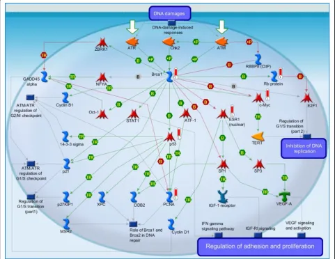
The 28 significant proteins in Figure 1(a) (see also Table 1) are significant proteins shared by the four can-cers, and these proteins and their PPIs form the com-mon core network markers of these four cancers. The significant proteins outside of these 28 are specific net-work markers, distinct for each cancer. Finally, based on these common core network markers and specific net-work markers, we investigated the mechanisms behind the carcinogenesis process with the help of databases (for example, GO database [23], DAVID database [24,25], and KEGG pathway database [26,27]) to find multiple network targets for cancer therapy. Unlike con-ventional theoretical methods that generate a single mathematical model for a cancer network for detailed theoretical analysis, ours is a systems biology approach to cancer network markers based on real microarray data through reverse engineering, theoretical statistical methods, and data mining in combination with big data-bases. These features made our method novel and helped produce the significant findings of our paper. The above paragraphs are adapted from our previous study [17] to make this paper to be a complete paper.

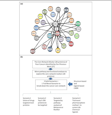
Several scenarios to break down the cancer core network

(6)

third approach by performing pathway analysis using Panther [28] and MetaCore (GeneGo Inc.) [29]. In addi-tion, we used a ‘confusion pharmacophore model’ to develop the fourth novel trial approach.

In the first approach, we chose the compounds with highest docking scores for each of the 28 significant pro-teins. Then we removed the redundant compounds, and

analyzed which compounds can target more than two pro-teins simultaneously. The basic strategy is to minimize the number of compounds necessary to target in order to break down the core network. Since there are 28 proteins in this core network, even choosing only one ligand to inhibit each of these 28 proteins would necessitate 28 ligands, which may be unsuitable for wet-lab validation.

(7)

In the second approach, we used the summation of the CRVs (Table 2 and Table 3) as the criterion to choose the key proteins to inhibit. In our previous study, we showed that CRV quantifies the extent of a protein’s association with other proteins, and thus it is optimal to target proteins with the highest summation of CRVs. This strategy depends on the cancer being tar-geted; in the present study, we focused on the common core network markers of the four cancers, so we chose the highest summation of CRVs across the four cancers.

In the third approach, we employed many new and valuable pathway analyses. Wet-lab cancer researchers can choose the pathway they want to focus on as the therapy target. There are many different combinations dependent on different conditions of cancers, so we do not list all the possibilities. Here, we demonstrate a sin-gle example, and others can develop their own scenarios following this example with the help of our docking results. (Additional file 4: Table S2)

The fourth novel approach is to develop confusion and individual pharmacophore models of core network

markers (28 proteins) to do virtual screening using the compounds stored in the Life Chemical database.

We highlight the different approaches in this section, because they form the crux of this study. Please see Fig-ure (1b). In the following sections, we describe the related methods necessary for each of the approaches.

More pathway and functional analyses

A. Panther

In our previous studies, we performed pathway analy-sis using the DAVID database. Here, we expand on the previous analysis by performing more pathway and func-tional analyses in order to develop a more efficient strat-egy for multiple target therapy. This approach will allow us to accumulate more information on possible therapy strategies. The 28 proteins comprising the cancer core network markers were analyzed for their molecular functions, molecular processes, and subcellular localiza-tions by the PANTHER (Protein ANalysis THrough Evolutionary Relationships) classification system [28]. PANTHER was designed to classify proteins (and their

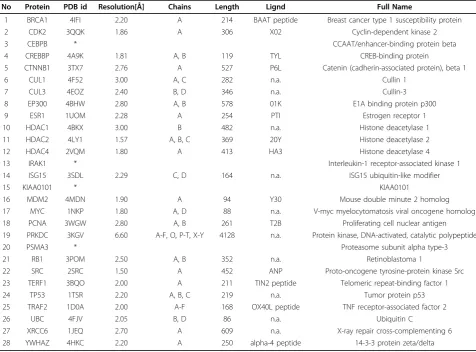
Table 1. Structure information of 28 core proteins

No Protein PDB id Resolution[Å] Chains Length Lignd Full Name

1 BRCA1 4IFI 2.20 A 214 BAAT peptide Breast cancer type 1 susceptibility protein

2 CDK2 3QQK 1.86 A 306 X02 Cyclin-dependent kinase 2

3 CEBPB * CCAAT/enhancer-binding protein beta

4 CREBBP 4A9K 1.81 A, B 119 TYL CREB-binding protein

5 CTNNB1 3TX7 2.76 A 527 P6L Catenin (cadherin-associated protein), beta 1

6 CUL1 4F52 3.00 A, C 282 n.a. Cullin 1

7 CUL3 4EOZ 2.40 B, D 346 n.a. Cullin-3

8 EP300 4BHW 2.80 A, B 578 01K E1A binding protein p300

9 ESR1 1UOM 2.28 A 254 PTI Estrogen receptor 1

10 HDAC1 4BKX 3.00 B 482 n.a. Histone deacetylase 1

11 HDAC2 4LY1 1.57 A, B, C 369 20Y Histone deacetylase 2

12 HDAC4 2VQM 1.80 A 413 HA3 Histone deacetylase 4

13 IRAK1 * Interleukin-1 receptor-associated kinase 1

14 ISG15 3SDL 2.29 C, D 164 n.a. ISG15 ubiquitin-like modifier

15 KIAA0101 * KIAA0101

16 MDM2 4MDN 1.90 A 94 Y30 Mouse double minute 2 homolog

17 MYC 1NKP 1.80 A, D 88 n.a. V-myc myelocytomatosis viral oncogene homolog

18 PCNA 3WGW 2.80 A, B 261 T2B Proliferating cell nuclear antigen

19 PRKDC 3KGV 6.60 A-F, O, P-T, X-Y 4128 n.a. Protein kinase, DNA-activated, catalytic polypeptide

20 PSMA3 * Proteasome subunit alpha type-3

21 RB1 3POM 2.50 A, B 352 n.a. Retinoblastoma 1

22 SRC 2SRC 1.50 A 452 ANP Proto-oncogene tyrosine-protein kinase Src

23 TERF1 3BQO 2.00 A 211 TIN2 peptide Telomeric repeat-binding factor 1

24 TP53 1TSR 2.20 A, B, C 219 n.a. Tumor protein p53

25 TRAF2 1D0A 2.00 A-F 168 OX40L peptide TNF receptor-associated factor 2

26 UBC 4FJV 2.05 B, D 86 n.a. Ubiquitin C

27 XRCC6 1JEQ 2.70 A 609 n.a. X-ray repair cross-complementing 6

28 YWHAZ 4HKC 2.20 A 250 alpha-4 peptide 14-3-3 protein zeta/delta

(8)

genes) in order to facilitate high-throughput analysis. It has a friendly user interface, you only need to input the gene list and set up the parameters, you will get the results you want. Please see Additional file 5: Figure S5.1 and the PANTHER website [28]

B. MetaCore

MetaCore includes a manually annotated database of gene interactions and metabolic reactions obtained from the scientific literature, including the most newly updated ones. The enrichment analysis of the biological process was based on the hypergeometric distribution algorithm and relevant pathway maps. The mathematical

Table 2. (a): CRVs of the 28 core proteins of each of the 4 cancers [17]

Protein Name Nam

CRV of Bladder Cancer

CRV of Liver Cancer

CRV of Colorectal Cancer

CRV of Lung Cancer

CRV SUM of 4 Cancers

Protein Name

CRV SUM (Sorted)

BRCA1 11.5863 6.8236 10.8636 12.5188 41.7923 UBC 496.3222

CDK2 16.7366 14.069 14.4739 9.942 55.2215 TP53 79.4445

CEBPB 5.2303 4.433 5.4262 7.2717 22.3612 KIAA0101 71.9887

CREBBP 12.0995 9.5856 11.5906 11.1892 44.4649 HDAC1 70.5646

CTNNB1 7.6796 9.5993 9.304 4.8015 31.3844 CDK2 55.2215

CUL1 13.2669 11.2802 5.5283 8.5044 38.5798 CUL3 53.8054

CUL3 13.0117 12.9519 16.3169 11.5249 53.8054 MYC 53.3347

EP300 12.1078 13.2218 8.3187 7.1278 40.7761 PCNA 52.9045

ESR1 5.6189 10.3758 6.3873 8.6696 31.0516 HDAC2 47.6069

HDAC1 19.2879 19.5736 11.7823 19.9208 70.5646 CREBBP 44.4649

HDAC2 11.0938 9.7752 18.9463 7.7916 47.6069 BRCA1 41.7923

HDAC4 5.8659 5.8397 9.7845 6.2225 27.7126 EP300 40.7761

IRAK1 4.1157 6.646 7.0177 5.1777 22.9571 CUL1 38.5798

ISG15 4.4856 6.0239 5.8124 4.943 21.2649 YWHAZ 35.9252

KIAA0101 15.8188 16.7663 19.1403 20.2633 71.9887 CTNNB1 31.3844

MDM2 4.5647 4.753 11.5648 6.2816 27.1641 ESR1 31.0516

MYC 13.0423 10.7821 20.0595 9.4508 53.3347 SRC 28.3907

PCNA 13.3217 15.1438 9.6282 14.8108 52.9045 TRAF2 27.7637

PRKDC 4.0781 5.9369 8.5589 5.6736 24.2475 HDAC4 27.7126

PSMA3 5.8022 7.7978 8.0875 5.2831 26.9706 MDM2 27.1641

RB1 6.8922 5.5531 5.9763 8.3205 26.7421 PSMA3 26.9706

SRC 8.8026 4.0767 9.1407 6.3707 28.3907 RB1 26.7421

TERF1 5.4642 4.9046 6.2595 8.0708 24.6991 XRCC6 25.7358

TP53 19.5883 18.7422 25.9329 15.1811 79.4445 TERF1 24.6991

TRAF2 9.2003 4.7703 7.365 6.4281 27.7637 PRKDC 24.2475

UBC 158.5321 137.284 80.3851 120.121 496.3222 IRAK1 22.9571

XRCC6 5.2871 9.5585 6.0231 4.8671 25.7358 CEBPB 22.3612

YWHAZ 8.7995 12.6421 7.9038 6.5798 35.9252 ISG15 21.2649

Table 3. (b) Top 5 ligands for the top 5 CRV proteins

UBC(4FJV) TP53(1TSR) KIAA0101 HDAC1(4BKX) CDK2(3QQK)

NCI Drug

LibDock Score NCI Drug

LibDock Score

719481 122.887 673172 126.112 655102 165.722 627865 134.685 680359 108.336

633409 114.187 695409 125.821 669588 164.036 625439 134.097 678636 101.875

672968 111.867 682236 117.725 407811 158.565 647638 125.505 669299 101.27

734999 111.578 695405 115.63 704564 148.676 2426 124.722 679065 101.006

(9)

foundation of MetaCore is shown in supplementary materials.

More pathway and functional analyses are fundamental to learning more about the hidden mechanisms of cancer networks. So, to interpret the results for the third approach in a meaningful way, this topic must be explained and described beforehand. The novelty of this paper is in its combination of systems biology with computer-aided drug design. Our research opens many new directions for multi-ple-target drug design; we describe only a portion of our results in this paper, for illustrative purposes. Our results clearly show that our approaches show great promise for future research to target special pathways through the design of drugs having multiple targets.

Metacore is also user-friendly software. The various man-uals and training materials can be download from public website [30,31], and due to the copyright concern, we do not copy too many material here. Please follow the instruc-tions in these manuals, and you can very well analysis. The mathematical foundation of Metacore is shown in Addi-tional file 6. Of course, the more deeply you understand the underlying statistics meaning, you can do better analysis.

Protein and ligand structures

The following section illustrates the computer-aided drug design (CADD) strategy applied to target the 28 common core network proteins. The first through third approaches need both the 3D structures of proteins and ligands, while the fourth pharmacophore approach only needs the structures of the ligands. The first thing we need is thus the 3D structures of the proteins. At this stage, 24 of them are available in the well-known PDB database, and we can download them directly, while there are four proteins (CEBPB, IRAK1, KIAA0101 and PSMA3) whose 3D structures have not been solved at this stage (Table 1). We used the NCI (46872 ligands) and Life Chemical (31742 ligands) drug libraries with the filter “anti-cancer”. The Developmental Therapeutics Program NCI/NIH offers the NCI-60 cell line screening. The users can download the 3D ligands (drugs) struc-tures from the website, and after the virtual screening, you can request them send you these drugs for free. Life Chemical is a commercial company, you have to pay to get these drugs [32]. All drug structures were prepared and minimized by Discovery Studio 3.5 (DS3.5). People seldom do the virtual screening on multiple targets since it is computationally intense. We performed this work on an IBM server with 160 cores and 1 TB of memory.

Homology model and binding site prediction

Proteins do not always have 3D structures available in the PDB database. Since only amino acid sequence data without corresponding structures were available for four of the proteins targeted in our study (CEBPB, IRAK1,

KIAA0101 and PSMA3) we used homology modeling to predict the structures for these proteins. Among many famous software and webservers, the I-Tasser webserver developed by Zhang et al. [33] is the most well-known homology modeling webserver. We used this server to perform homology modeling of our proteins of interest that lacked available 3D structures. For some well-studied protein targets, structures with embedded ligands are available, so the exact binding site for the docking experiments is known. However, binding site information was unavailable for most proteins, so we used the COACH webserver [34], also developed by Zhang et al., to predict the binding sites. The detailed binding site information is shown in Additional File 7. I-TASSER and COACH are both user friendly webser-ver. You only need to input the sequence of protein residue into the I-TASSER, and set up the parameters, it will give you the predicted 3D protein structures. Users input the 3D protein structures into the COACH and set up the parameters, and then it will give you the pre-dicted binding sites (Additional file 5: Figure S5.2, S5.3).

Docking

After prepared the 3D structures of proteins and ligands, and find out the binding site, we can perform docking for virtual screening. We used DS 3.5 to per-form docking simulations, and then ranked the docking results based on LibDock score. We chose the top 20 compounds for further analysis, such as the construction of pharmacophore models. The DS 3.5 is also user friendly software, users can download the manual from website, please see the example for parameter setting of docking. Please see Additional file 5: Figure S5.4

Pharmacophore Model

A. HypoGen method and virtual screening

(10)

traditional one. As mentioned above, this is a novel idea, and the pharmacophore model is just a prototype: it will require further modification in future studies. In tradi-tional pharmacophore modeling, the IC50value for each

drug under investigation is necessary, but our model does not require them. Instead, we linearly transformed LibDock scores to generate putative IC50values, and

used these values to build the pharmacophore. We com-bined the top three ligands for each of the 28 proteins to make a ligand pool, and then used this ligand pool to construct a common pharmacophore; this is qualitatively different from building 28 individual pharmacophores. We build the Hypogen model by the DS 3.5, and it is also user friendly. However, to build a correct Hypogen model is a time consuming work, you need to try the different combination of compounds. For a skill expert with nor-mal computational resource, it often needs at least one month to build the correct model. We show the user interface for detailed parameter setting for your refer-ence. Please refer to Additional file 5 : Figure S5.5.

B. PharmaGist

PharmaGist is another method to construct ligand-based pharmacophores. Because it does not require IC50

values of ligands [35], it is easier to construct pharmaco-phores by PharmaGist than by the HypoGen model. For each protein, we constructed one PharmaGist model: these models can be used to do virtual screening in the future. PharmaGist is also a user friendly webserver. Please see Additional file 5: Figure S5.6.

Cocktail multiple-target strategy: A novel model combined with systems biology and CADD

In summary, we used systems biology to construct the common core network marker of four different cancers, which contains 28 proteins as the house-keeping proteins shared by the different cancers. Then we used the dock-ing and pharmacophore methods to perform virtual screening on these 28 core proteins and get the top com-pounds for each protein. In contrast to traditional single target methods, we suggest using a combination of the top compounds to perform cell proliferation experi-ments. We have provided an example for each of our first three approaches. Our research provides a novel direction for target therapy for cancers. Wet-lab biomedi-cal scientists can combine the top ligands for each of the 28 core proteins based on their experimental conditions and the pathways that they want to focus on. As an early stage project, we have taken a conservative approach, only using the NCI anti-cancer drug library. As these drugs have proven anti-cancer activity, our cocktail of multiple drugs can be expected to slightly or moderately enhance the therapeutic effect under the right wet-lab conditions. Collaboration with and input from wet-lab experts would permit the modification and optimization

of our model, and the scope could expand to include other drug libraries in the virtual screening.

Biological Experimental Validations

The detailed protocol for the biological experiment in this Part, please refer to our previous work [36]. And the results please refer to Additional file 8. Recently, our team members who are part of wet-lab experiments have found that: if we used more than one drug to attack more than one target at the same time, it will decrease the IC50of the drug. Our team has shown that

if we used Gefitinib (Iressa) and L4 (one drug from the LOPAC drug library) to inhibit Src and EGFR at the same time, we achieve lower cell viability.

Results and Discussion

Review of the results of our previous methods

Our previous study identified 28 core proteins in the common core network marker for four cancers [17]. These are the proteins intersecting between the four cancers’ PPI networks with the top CRVs. Figure 1(a) shows the PPI information of each common core net-work marker. As stated previously, these 28 core pro-teins could be responsible for the house-keeping mechanisms of these four cancers, so using the mini-mum possible number of ligands to target the maximini-mum possible number of the 28 proteins could be the most efficient strategy to attack the cancers.

Several approaches to break the cancer core network marker

a. We chose the top 20 compounds with the highest docking scores for each of the 28 significant proteins. Of a total of 560 ligands (Additional file 4: Table S2), we found there were 13 ligands that target 2 or 3 pro-teins simultaneously (Table 4(a)) after redundancy ana-lysis. These 13 ligands combined 11 target proteins (Table 5new 3(b)). We used the 13 ligands as the mini-mum package for breaking the core network by inhibit-ing these 11 proteins. While this does not target all 28 proteins, the main purpose here was to minimize the number of ligands at this first stage trial. (As we have said, this is the first trial of our primary model.) Of course, according to our docking results of these 28 pro-teins, there are thousands of possible drug combinations that can be used based on different analysis methods as per a given researcher’s scope. It is quite possible to develop combinations to target all the 28 proteins based on our docking results.

(11)

be the therapeutic targets for breaking cancer core net-work marker. According to our previous systems biology analysis, we believe that inhibiting proteins with the

highest CRVs is a highly efficient way to attack cancers. As the first trial, our combination of proteins with the top 5 CRVs should simply be taken as a proof of concept: one can develop combinations according to one’s particular needs based on our CRVs.

c. We have also listed pathway analyses using Panther and MetaCore on the core network proteins. Other scientists can use this information to choose the path-ways that they want to target, and then choose the best combination of drugs from our virtual screening results. For instance, from the pathway analysis results using Panther (Table 6), researchers interested in targeting the p53 pathway can choose between EP300, CREBBP, HDAC1, HDA2, TRAF2, CDK2, MDM2, and TP53 as the therapy targets. For the above scenario, researchers can choose the top drugs from Additional file 4: Table S2. MetaCore gives us more information for the purpose of target therapy. The top three modules mapped to our 28 core proteins are listed in Table 7. Taking the first map/ module (DNA damage_ATM/ATR regulation of G1/S checkpoint) as an example, we see CDK2, p53, Ubiquitin, BRCA1, c-Myc, PCNA, and MDM2 are related to this module. As above, we can use the drugs in Additional file 4 : Table S2 to choose the optimal combination of drugs to attack this module.

More pathway and functional analysis

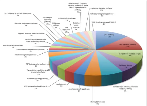
A. Panther

The results of Panther are shown in Figure 2 and listed in Table 6. We see the 28 core network markers hit many important cancer-related pathways, such as p53, Wnt signaling, p53 feedback loops 2, apoptosis,etc. As we have described above, this study is a prototype model. Inhibition of the right proteins hitting the key pathways is an important strategic consideration in real clinical situations. Our results offer another reference for doctors to design the best combination of multiple inhibitors. In the future, using clinical data from doctors will help us perform deeper analysis. These preliminary results also could help us exclude pathways unrelated to cancer at the first stage, such as those related to Hun-tington’s disease, Alzheimer’s disease,etc.

B. MetaCore

The results of MetaCore analysis are described below. We have described the top three maps/modules (Table 7).

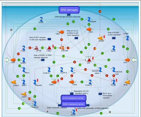
(i) DNA damage_ATM/ATR regulation of G1/S checkpoint (Figure 3): It is the highest scoring map (i.e., the map with the lowest p value). ATM/ATR regulates both the checkpoints of the G1/S and S/G2. DNA damage checkpoints pathways arrest or delay the pro-gression of cell cycle in response to the DNA damage. Eukaryotic cell cycle have four phases, G1 (G indicating gap), S (Synthesis), G2 (Gap 2), and M (Mitosis), and one outside, G0 (Gap 0) [37]. When DNA damage

Table 4. NCI drugs target more than one protein

NO. NCI Drug Protein Name LibDock Score

1 625439 KIAA0101 145.708

625439 HDAC1(4BKX) 134.097

625439 HDAC4(2VQM) 149.324

2 645378 CEBPB(2E_42) 158.637

645378 KIAA0101 140.103

3 668448 BRCA1(4IFI) 192.069

668448 PSMA3 166.516

4 668577 MYC(1NKP) 125.603

668577 PSMA3 180.11

5 682094 TERF1(3BQO) 123.287

682094 YWHAZ(4HKC) 182.534

6 687363 MYC(1NKP) 145.138

687363 YWHAZ(4HKC) 184.649

7 695175 TRAF2(1D0A) 101.267

695175 PSMA3 148.83

8 695409 TP53(1TSR) 125.821

695409 PSMA3 164.906

9 704565 KIAA0101 137.38

704565 HDAC4(2VQM) 153.564

10 719660 MYC(1NKP) 134.021

719660 YWHAZ(4HKC) 200.903

11 724305 CEBPB(2E_42) 167.724

724305 HDAC4(2VQM) 141.195

12 726771 BRCA1(4IFI) 142.956

726771 HDAC4(2VQM) 148.366

13 742856 MYC(1NKP) 140.093

742856 TP53(1TSR) 100.787

Table 5. The proposed 13 drugs totally target the following 11 proteins

No. Protein Name

1 BRCA1(4IFI)

2 CEBPB(2E42)

3 ISG15(3SDL)

4 MDM2(4MDN)

5 PCNA(3WGW)

6 PRKDC(3KGV)

7 PSMA3

8 SRC(2SRC)

9 TERF1(3BQO)

10 TP53(1TSR)

(12)

occurs, the G1/S checkpoints will inhibit the initiation of replication to prevent cells from entering the S phase. They are related to two pathways of signal transduction, to initiate and maintain the G1/S arrest, respectively [37]. Jiri Bartek et al. discussed “The DNA damage response in tumorigenesis and the treatment of cancer” [38]. [The above description is directly cited from the Metacore document.]

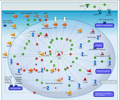
(ii) Transcription_P53 signaling pathway (Figure 4): It is the second highest scoring map (i.e., the map with the second lowest p-value). The Tumor protein p53,

also known as p53 ortransformation-related protein 53 (TRP53), acts a significant role in shielding the genome integrity. While being activated, p53 will bind to the enhancer/promoter regions of downstream target genes. And then it regulates the transcription of these genes, through which it initiates cellular processes that responsible for lots of its tumor-suppressor related functions [39]. It is not surprising that core network of 4 cancers are related to the p53 signaling pathway. [The above description is directly cited from the Meta-core document.]

Table 6. the pathway analysis results of Panther

Rank Pathway title Count Gene

1 p53 pathway 8 EP300,CREBBP,HDAC1,HDA2,TRAF2,CDK2,MDM2,TP53

2 Wnt signaling pathway 7 EP300,CREBBP,HDAC1,MYC,HDAC2,CTNN1,TP53

3 p53 pathway feedback loops 2 6 MYC,RB1,CTNNB1,CDK2,MDM2,TP53

4 Parkinson disease 4 YWHAZ, CUL1,PSMA3,SRC

4 Gonadotropin releasing hormone receptor pathway 4 EP300,CREBBP,CTNNB1, SRC

5 Huntington disease 3 EP300,CREBBP,TP53

6 Apoptosis signaling pathway 2 TRAF2,TP53

6 Angiogenesis 2 CTNNB1, SRC

6 P53 pathway feedback loops 1 2 MDM2, TP53

6 Cadherin signaling pathway 2 CTNNB1, SRC

6 Transcription regulation by bZIP transcription factor 2 EP300, CREBBP

6 TGF-beta signaling pathway 2 EP300, CREBBP

7 Interleukin signaling pathway 1 MYC

7 Alzheimer disease-presenilin pathway 1 CTNNB1

7 Integrin signalling pathway 1 SRC

7 Insulin/IGF pathway-protein kinase B signaling cascade 1 MDM2

7 Hypoxia response via HIF activation 1 CREBBP

7 Ubiquitin proteasome pathway 1 MDM2

7 p53 pathway by glucose deprivation 1 TP53

Please see their statistical distribution in Figure 2.

Table 7. Top three modules/maps given by Metacore

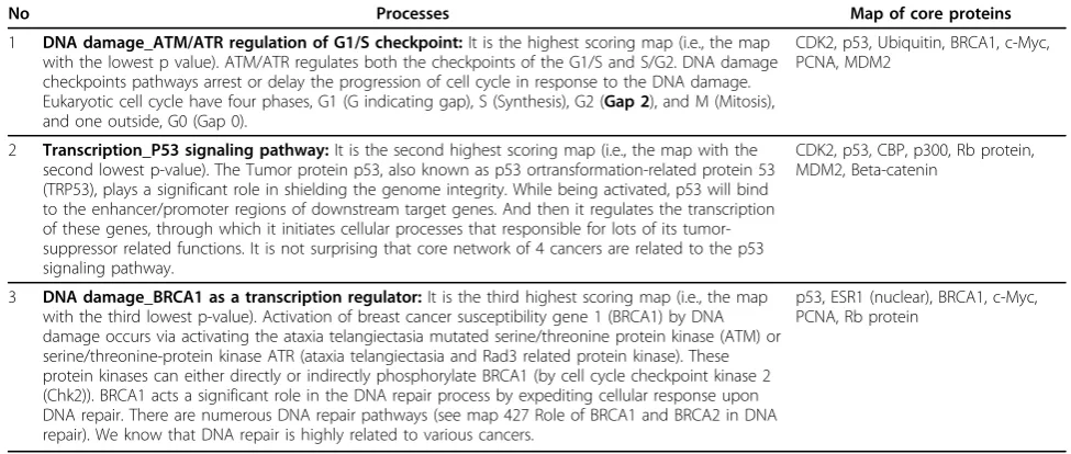
No Processes Map of core proteins

1 DNA damage_ATM/ATR regulation of G1/S checkpoint:It is the highest scoring map (i.e., the map with the lowest p value). ATM/ATR regulates both the checkpoints of the G1/S and S/G2. DNA damage checkpoints pathways arrest or delay the progression of cell cycle in response to the DNA damage. Eukaryotic cell cycle have four phases, G1 (G indicating gap), S (Synthesis), G2 (Gap 2), and M (Mitosis), and one outside, G0 (Gap 0).

CDK2, p53, Ubiquitin, BRCA1, c-Myc, PCNA, MDM2

2 Transcription_P53 signaling pathway:It is the second highest scoring map (i.e., the map with the second lowest p-value). The Tumor protein p53, also known as p53 ortransformation-related protein 53 (TRP53), plays a significant role in shielding the genome integrity. While being activated, p53 will bind to the enhancer/promoter regions of downstream target genes. And then it regulates the transcription of these genes, through which it initiates cellular processes that responsible for lots of its tumor-suppressor related functions. It is not surprising that core network of 4 cancers are related to the p53 signaling pathway.

CDK2, p53, CBP, p300, Rb protein, MDM2, Beta-catenin

3 DNA damage_BRCA1 as a transcription regulator:It is the third highest scoring map (i.e., the map with the third lowest p-value). Activation of breast cancer susceptibility gene 1 (BRCA1) by DNA damage occurs via activating the ataxia telangiectasia mutated serine/threonine protein kinase (ATM) or serine/threonine-protein kinase ATR (ataxia telangiectasia and Rad3 related protein kinase). These protein kinases can either directly or indirectly phosphorylate BRCA1 (by cell cycle checkpoint kinase 2 (Chk2)). BRCA1 acts a significant role in the DNA repair process by expediting cellular response upon DNA repair. There are numerous DNA repair pathways (see map 427 Role of BRCA1 and BRCA2 in DNA repair). We know that DNA repair is highly related to various cancers.

(13)

(iii) DNA damage_Brca1 as a transcription regulator (Figure 5): It is the third highest scoring map (i.e., the map with the third lowest p-value). Activation of breast cancer susceptibility gene 1 (BRCA1) by DNA damage occurs via activating the ataxia telangiectasia mutated serine/threonine protein kinase (ATM) [40] or serine/ threonine-protein kinase ATR (ataxia telangiectasia and Rad3 related protein kinase) [41]. These protein kinases can either directly or indirectly phosphorylate BRCA1 (by cell cycle checkpoint kinase 2 (Chk2) [42]). BRCA1 acts a significant role in the DNA repair process by expediting cellular response upon DNA repair. There are numerous DNA repair pathways (see map 427 Role of BRCA1 and BRCA2 in DNA repair) [43]. We know that DNA repair is highly related to various cancers. [The above description is directly cited from the Meta-core document.]

* The highest three scoring map (i.e., the map with the three lowest p-value) is based on the enrichment distri-bution sorted by the‘Statistically significant maps’set. Experimental data from all files is linked to and visualized on the maps as thermometer-like figures. Up-ward ther-mometers are red and indicate up-regulated signals, and down-ward (blue) ones indicate down-regulated expres-sion levels of the genes. [The above description is directly cited from the Metacore document.]

Statistical analysis results of the three maps are shown in Table 7. These results also help us choose more sui-table targets and exclude less suisui-table ones.

Protein and ligand structures

Table 1 shows detailed information of these 28 proteins including protein name, PDB ID, resolution, chains, length, ligands, and their full names. Most of these 3D

(14)

structures were downloaded from the PDB database. 3D structures of CEBPB, IRAK1, KIAA0101 and PRKDC were constructed by homology modeling using I-TAS-SER. We can see that many protein structures also con-tained a ligand in a bound conformation. We used the locations of these ligands within the target protein as the docking site. Binding sites of proteins without bound ligands were predicted using COACH.

Docking

Figure 6 Additional file 9 shows the docking pose of the top compounds (i.e., those with the highest docking score). Their docking scores ranged from 95 to 241. The analysis also shows the key residues in ligand binding. Our study is the first to perform high-throughput

multiple-protein docking, and this work requires large computational resources. Due to space limitations, we have not listed another table for these key residues. The information could be useful for future drug design and these top compounds could be considered as con-trol ligands.

Pharmacophore

3D pharmacophore modeling is another powerful method to perform virtual screening on large ligand databases. It is as powerful as the docking method, and is always more efficient than docking methods. For example, the large ligands database ZINC [44] has more than 200 million ligands. By calibrating the parameters of the pharmacophore virtual screening, it is possible to

(15)

virtually screen the whole ZINC database using our IBM server with 160 cores. We have even performed virtual screening for Src inhibitors. However, constructing a proper HypoGen model is also very time-consuming. As an initial study using a novel approach, we used relatively unrestricted conditions to set up a rough HypoGen model. It would be beneficial to do virtual screening on another ligand database in the future.

Figure 7 Additional file 10 lists the total 54 ligands used to construct the HypoGen pharmacophore model. We present the structure of the pharmacophore in Figure 6 new, where NSC-625869 refers to the ligand in the NCI library of anti-cancer drugs that was screened and matched by this pharmacophore. The numerical results of

the HypoGen model are shown in Tables 8, 9, 10. After having constructed this pharmacophore, we were able to use it to screen against other ligand databases, such as the Life Chemical database. Figure 7 and Table 11new show the compounds in the Life Chemical database screened and matched by this pharmacophore. Compared to the HypoGen model, the pharmacophore model derived by PharmGist is easier to obtain because PharmGist does not require the IC50values of the compounds for

computa-tion. We have listed the results in Figure 8 and Table 12.

Biological Experimental Validations

Drug combination- Gefitinib (Iressa) combine with L4 and N4 in three different cells. In the three cell lines,

(16)

they show that combination drug always get a better efficiency that only single Iressa. Please refer to Addi-tional file 8. At this stage, we have only used a simple pathway diagram to visualize the relationship between EGFR and Src without a large-scale systems biological analysis. These results gave us confidence that multiple drugs attacking multiple targets will achieve better results. Indeed, we have accumulated lots of similar results.

Novel model combined with both systems biology and CADD

· General demonstration: Our method has reversed the normal procedure of CADD with the help of systems biology. In the traditional CADD method, a single

validated target, such as Src, EGFR, and FAK, is used as the protein target. The first step is usually virtual screening by docking or the pharmacophore method. The second step is to validate the top compounds from virtual screening with ELISA or Western blot wet-lab experiments. If they are found to bind to the target pro-teins, then researchers could employ these ligands in cell proliferation experiments. For our novel approach, we choose the top compounds from several targets simultaneously, and then perform the cell proliferations experiment at the beginning. Our hypothesis is that these drug cocktails would destroy the core network, although we have not experimentally validated whether each top compound binds to its corresponding target or not

(17)

Figure 6new 8- The hypogen pharmacophore model built by DS3.5. We show the distances between the pharmacophores. No. 625869 is the drug in NCI anti-cancer library screened and matched by this pharmacophore.

(18)

Table 8. Top pharmacophore description

Category Number of ligands IC50range (nM)

Feature Correlation

28 targets 54 2-50000 HBA, HBA, HY, RA 0.92

Table 9. Top 10 pharmacophore descriptions

Hypothesis Total cost ΔCost RMS Correlation (r) Features

1 211.414 33.787 0.583549 0.924995 HBA, HBA, HY, RA

2 211.745 33.456 0.599912 0.920410 HBA, HBA, HY, RA

3 212.295 32.906 0.606595 0.918758 HBA, HBA, HY, RA

4 212.530 32.671 0.609627 0.917975 HBA, HBA, HY, RA

5 213.564 31.637 0.641692 0.908625 HBA, HBA, HY, RA

6 213.870 31.331 0.651935 0.905497 HBA, HBA, HY, RA

7 214.412 30.789 0.669021 0.900153 HBA, HBA, HY, RA

8 215.039 30.162 0.690558 0.893115 HBA, HBA, HY, RA

9 215.282 29.919 0.694361 0.891929 HBA, HBA, HY, RA

10 215.758 29.443 0.713440 0.885327 HBA, HBA, HY, RA

* Null cost = 245.201; Fixed cost = 202.014; Configuration cost = 19.2545;ΔCost = Null cost - Total cost. All costs are in units of bits. * HBA, hydrogen bond acceptor; HY, hydrophobic; RA, ring aromatic.

Table 10. Experimental and estimation values of IC50for each of the 54 ligands

NCI Drug IC50(nM) Error NCI Drug IC50(nM) Error

Exp. Est. Exp. Est.

625869 2.0 2.4 1.2 669299 4792.2 5656.4 1.2

668448 66.3 142.2 2.1 641847 5026.9 4480.2 -1.1

698233 256.5 97.5 -2.6 669230 5282.5 4302.8 -1.2

668433 380.2 229.7 -1.7 657381 5358.4 4451.3 -1.2

737026 810.9 366.4 -2.2 643737 5376.8 4463.6 -1.2

654626 1377.0 1868.5 1.4 691369 5509.1 4822.7 -1.1

726771 1877.1 4272.0 2.3 627399 5527.5 4285.1 -1.3

717079 2067.7 4413.1 2.1 627727 5892.9 14154.0 2.4

674086 2234.0 4138.9 1.9 693235 6107.2 5310.1 -1.2

666346 2270.0 5579.5 2.5 675823 6377.0 5049.0 -1.3

740601 2627.9 4280.5 1.6 665675 6591.5 4380.4 -1.5

639795 2742.6 4358.1 1.6 295632 7254.4 4402.1 -1.6

673172 2823.0 4721.0 1.7 668373 7390.1 4343.3 -1.7

641236 2827.4 4418.8 1.6 749 7534.5 21062.2 2.8

76955 2836.7 4936.6 1.7 689447 8003.5 5397.9 -1.5

719481 3033.7 6903.6 2.3 202537 12700.6 21711.5 1.7

406433 3064.1 12371.9 4.0 639906 13142.7 5880.0 -2.2

683481 3344.0 4540.1 1.4 622153 14753.4 5742.3 -2.6

682236 3395.0 4677.1 1.4 622154 15831.2 4771.3 -3.3

661908 3469.7 4310.7 1.2 692400 50000.0 13059.1 -3.8

633409 3661.4 4382.2 1.2 687325 50000.0 14121.3 -3.5

672968 3845.3 4363.1 1.1 689530 50000.0 17997.5 -2.8

680359 4140.3 4290.9 1.0 691200 50000.0 21974.7 -2.3

76519 4334.6 3133.5 -1.4 684143 50000.0 32999.6 -1.5

702125 4732.2 4288.4 -1.1 683630 50000.0 40400.2 -1.2

678636 4732.9 12631.9 2.7 694265 50000.0 51746.7 1.0

682086 4770.1 4479.7 -1.1 695571 50000.0 61122.2 1.2

(19)

· Time complexity versus space complexity:Our novel approach is some kind like the problem of algorithm about the time complexity and space complexity. To attack each protein one by one is similar to the problem of time com-plexity. This is the traditional strategy for single target drug design. The traditional method needs to make sure the drugs target to which protein exactly. In the language of computer science, the traditional CADD method can only do serial work but not parallelization work. By the help of our systems biology approach, it turns the origin problem from time complexity to space complexity. That is, you can do parallelization attack to the multiple proteins simulta-neously. The powerful of this parallelization attack is that you can do various drugs combination trial at the short time. When you get the better results, you can go back to check each drug in the combination is useful for the pro-teins individually or not. Honest to speak, there are possi-ble too many uncertainties and inaccuracies in this model, such as the network biomarkers predicted by our systems biology approach, the binding site information, the phar-macophore model or even the predicted 3D protein struc-tures. However, due to the powerful of parallelization attack (cocktail multiple drugs), it is possible to find the useful cocktail combination under the situation of so many uncertainties and inaccuracies. The problem of space com-plexity we encounter now is that how many drugs we could use at the same time. And this is our feature work.

· Welcome to asking for our help and cooperation:

We must emphasize that no matter how powerful of our model, the most important thing is to combine with the

correct medical knowledge and intuition. After our model gives so many possible combinations of drug, you have to decide a set of best ones with your medical knowledge and intuition to do the wet-lab experiment validation. We already have a lot of these wet-lab results but not pub-lished yet. Our teams also have abundant experience on the single target drug design [45-47]. We have also built a webserver of the systems biology model in the research but not opened to public yet. It is welcome for your feed-back and cooperation. You are welcome to modify the old version source code of our systems biology model [48]. Please refer to Additional file 8.

· Novelty and expectation results in the future: Com-bination drugs is not a novel idea [49,50]. To design com-bination drugs by our systems biology and CADD methods is a novel work. We expect many combination drugs will be really useful by the help of model. We would like to enhance and modify our model in the future.

Availability of this method

We are in the process of building a webserver to iden-tify network biomarkers. At this stage, we can construct the network on request. We also offer a working version of the source code (Additional File 11), and the readers can modify this version of source code to perform their research experiments.

Conclusions

In this study, we combined systems biology with tradi-tional computatradi-tional-aided drug design to design drug

Table 11. The Life-Chemical ligands are virtually screened by the hypogen model

ID No. FitValue Estimate HBA_1 HBA_2 HY_3 RA_4

F0325-0146 6.580 4.599 1 1 1 1

F0289-0199 6.446 6.266 1 1 1 1

F0922-0370 5.935 20.327 1 1 1 1

F0012-0228 5.690 35.775 1 1 1 1

F0496-0019 5.623 41.719 1 1 1 1

F0737-0405 5.55006 49.3217 1 1 1 1

F0382-0020 5.53538 51.0174 1 1 1 1

F0325-0148 5.1207 132.555 1 1 1 1

F0737-0312 5.00395 173.442 1 1 1 1

F0725-0356 4.98991 179.137 1 1 1 1

F0301-0263 4.9208 210.04 1 1 1 1

F0473-0314 4.90716 216.74 1 1 1 1

F0922-0913 4.87165 235.207 1 1 1 1

F1601-0068 4.58408 456.055 1 1 1 1

F0463-0195 4.50862 542.605 1 1 1 1

F0866-0317 4.26226 956.832 1 1 1 1

F0537-0936 4.17732 1,163.54 1 1 1 1

F0180-0144 3.96884 1,880.45 1 1 1 1

F0922-0900 3.95736 1,930.82 1 1 1 1

(20)

cocktails to inhibit the 28 proteins that comprise the common core network markers of four cancers. The results of our previous study have led us to believe that those proteins likely represent house-keeping proteins of

these four cancers. Wet-lab researchers could use the cocktails of multiple drugs indicated by our analysis as objects of study in experiments on treating the four can-cers. Moreover, with the help of sensitivity analysis, we

(21)

also found the most likely multiple drug targets for each individual cancer.

Additional material

Additional file 1: Parameter Identification of PPI network by Maximum Likelihood Method.

Additional file 2: Determination of significant protein associations by AIC and Student’s t-test.

Additional file 3: The identified significant proteins in 4 cancers.

Additional file 4: Docking results for the top 20 ligands for the 28 proteins studied.

Additional file 5: new 6: User interface of commercial software and free webserver.

Additional file 6: new 7: Mathematical foundation of Metacore.

Additional file 7: new 5: Binding site information for the 28 proteins.

Additional file 8: new 10: Biological experimental validation.

Additional file 9: new 8. Docking pose analysis of 28 core proteins. The docking poses analysis shows the key residues of the proteins which interact with the ligands. The analysis reveals more mechanisms to help us designde novodrugs.

Additional file 10: new 9. 54 ligands used for developing the Hypogen model.

Additional file 11: Source code (*.rar).

Competing interests

The authors declare that they have no competing interests.

Authors’contributions

BSC and YHW designed and conduct the theory and experiments of systems biology. CWL modified the core network. JC, YHW, CLL and TSC design and perform the CADD. JC, CAC, PSJ and YHL design and perform the wet-lab biological experiments. LJC perform the pathway and functional analysis. BSC and YHW integrated the whole work. YHW drafted the manuscript. All of the authors have approved the publication of the manuscript.

Acknowledgements

The authors are grateful for the support provided by the Ministry of Science and Technology, Taiwan through grants MOST-103-2745-E-007-001-ASP, MOST-103-2221-E-038 -013 -MY2, and MOST-104-2218-E-007-021.

Declaration

Funding for this publication was provided by the Ministry of Science and Technology, Taiwan through grants 103-2745-E-007-001-ASP, MOST-103-2221-E-038 -013 -MY2, and MOST-104-2218-E-007-021.

Table 12. The pharmacophores descriptions of PharmGist

No. Protein PDB Score Features Spatial Features R H D A N P Chemicals Fig

1 BRCA1 4IFI 39.2 7 7 4 0 0 2 0 1 3 9-1

2 CDK2 3QQK 33.1 5 5 4 0 0 1 0 0 3 9-2

3 CEBPB 2E42 40.4 12 12 3 5 0 4 0 0 3 9-3

4 CREBBP 4A9K 29.9 5 5 1 0 2 2 0 0 9 9-4

5 CTNNB1 3TX7 23.7 3 3 2 0 0 1 0 0 7 9-5

6 CUL1 4F52 37.5 7 7 4 1 0 2 0 0 3 9-6

7 CUL3 4EOZ 25.7 5 5 2 0 0 3 0 0 3 9-7

8 EP300 4BHW 3.0 2 2 0 0 0 2 0 0 2 9-8

9 ESR1 1UOM 33.1 5 5 4 0 0 1 0 0 3 9-9

10 HDAC1 4BKX 26.5 4 4 3 0 0 0 0 1 4 9-10