https://doi.org/10.5194/gmd-10-3547-2017 © Author(s) 2017. This work is distributed under the Creative Commons Attribution 3.0 License.
Implementation of a physically based water percolation routine in
the Crocus/SURFEX (V7.3) snowpack model
Christopher J. L. D’Amboise1,2, Karsten Müller1, Laurent Oxarango3, Samuel Morin4, and Thomas V. Schuler2
1Norwegian Water Resources and Energy Directorate, Oslo, 0368, Norway 2Department of Geoscience, University of Oslo, Oslo, 0316, Norway 3Univ. Grenoble Alpes, CNRS, IRD, IGE, 38000 Grenoble, France
4Météo-France – CNRS, CNRM UMR 3589, Centre d’Etudes de la Neige, Grenoble, France
Correspondence to:Christopher J. L. D’Amboise ([email protected]) Received: 7 March 2017 – Discussion started: 10 April 2017
Revised: 14 August 2017 – Accepted: 18 August 2017 – Published: 26 September 2017
Abstract.We present a new water percolation routine added to the one-dimensional snowpack model Crocus as an alter-native to the empirical bucket routine. This routine solves the Richards equation, which describes flow of water through unsaturated porous snow governed by capillary suction, grav-ity and hydraulic conductivgrav-ity of the snow layers. We tested the Richards routine on two data sets, one recorded from an automatic weather station over the winter of 2013–2014 at Filefjell, Norway, and the other an idealized synthetic data set. Model results using the Richards routine generally lead to higher water contents in the snow layers. Snow layers of-ten reached a point at which the ice crystals’ surface area is completely covered by a thin film of water (the transition between pendular and funicular regimes), at which feedback from the snow metamorphism and compaction routines are expected to be nonlinear. With the synthetic simulation 18 % of snow layers obtained a saturation of >10 % and 0.57 % of layers reached saturation of >15 %. The Richards rou-tine had a maximum liquid water content of 173.6 kg m−3 whereas the bucket routine had a maximum of 42.1 kg m−3. We found that wet-snow processes, such as wet-snow meta-morphism and wet-snow compaction rates, are not accu-rately represented at higher water contents. These routines feed back on the Richards routines, which rely heavily on grain size and snow density. The parameter sets for the wa-ter retention curve and hydraulic conductivity of snow layers, which are used in the Richards routine, do not represent all the snow types that can be found in a natural snowpack. We show that the new routine has been implemented in the Cro-cus model, but due to feedback amplification and parameter
uncertainties, meaningful applicability is limited. Updating or adapting other routines in Crocus, specifically the snow compaction routine and the grain metamorphism routine, is needed before Crocus can accurately simulate the snowpack using the Richards routine.
1 Introduction
meteorological and hydrological observations with physi-cally based percolation modeling. A physiphysi-cally based water percolation model has been used along with weather station data to improve forecasts of wet-snow stability (Wever et al., 2016a) and determine initial conditions for simulations of avalanche dynamics (Vera Valero et al., 2016).
Vertical water flow through a layered snowpack can oc-cur in two different modes, matrix flow and preferential flow. Matrix flow is a diffusive flow through the pore space of the snowpack, which sets up a uniform water front. Preferential flow, also called finger flow, is when water quickly flows in channels to deeper layers (Marsh and Woo, 1984). A com-bination of both flow schemes occurs in a snow layer; often preferential flow will initiate wetting a dry snow layer, fol-lowed by an expansion of flow paths that will end up in ma-trix flow (Williams et al., 2010). As water percolates through an isothermal snowpack, preferential flow paths are created, and water transport through the snowpack becomes very ef-ficient (Colbeck, 1979). Using multicolored dye tracer ex-periments, Schneebeli (1995) has shown that the preferential flow channels in an isothermal snowpack can migrate over time.
Gravity and capillary forces govern water movement in unsaturated snow (Colbeck, 1972; Jordan et al., 1999). Cap-illary forces arise from adhesion and surface tension of liquid water inside the pore space of the snowpack. Snow layering produces vertical gradients since capillary pressure has an inverse relationship to pore size (Wankiewicz, 1978). Pres-sure gradients acting against gravity may induce the forma-tion of preferential flow channels, as flow channels in soil occur where capillary pressure gradient opposes the water flow direction (Philip, 1975). Two common textural barri-ers are crust laybarri-ers and neighboring snow laybarri-ers with sharp grain size differences. Assessing the hydraulic conductivity of textural barriers is not straightforward, because layer be-havior may vary greatly; for example, crusts can act as an impermeable layer or act similar to vertical conduits (Jor-dan, 1995). Fine-grained snow layered above coarser grains gives rise to flow barriers due to capillary pressure gradients opposing gravity. An area of high saturation can be found above such barriers and lateral water flow due to suction, ter-rain slope and water pooling is a common result (Colbeck, 1974b; Williams et al., 2010).
Physically based models of water percolation through snow were first developed to describe gravitationally driven flow through isotropic isothermal snow, neglecting capil-lary effects (Colbeck, 1972). Model complexity evolved and snow layering was introduced (Colbeck, 1974b, 1975), as well as heterogeneous flow where water is routed to deeper layers via flow channels (Colbeck, 1979). Further improve-ment in modeling percolation in cold snowpacks was ad-dressed by including thermodynamics into percolation mod-els (Bengtsson, 1982; Colbeck, 1976; Illangasekare et al., 1990). Capillary forces were introduced in some early mod-els despite the deficiency in parameter sets (Colbeck, 1974a;
Jordan, 1983; Wankiewicz, 1978). Wankiewicz (1978) con-cluded that more information on snow microstructure is needed to improve modeling of water percolation through a layered snowpack. Some recent models include gravity and suction-driven, preferential flow in isothermal snow layers (Hirashima et al., 2014; Katsushima et al., 2009).
Measuring the hydraulic conductivity and water retention of snow layers is a time-consuming task performed in a cold lab. It cannot currently be conducted in the field or even de-ployed as an autonomous recording system. Yet, new param-eterizations of the retention curve (Yamaguchi et al., 2010, 2012) and permeability, which relates to hydraulic conduc-tivity (Calonne et al., 2012), have been developed recently. These developments have been utilized in percolation mod-els based on Darcy’s law (Hirashima et al., 2010) and the Richards equation (Wever et al., 2014, 2015). Hydraulic con-ductivity and water retention of snow layers give insight into how the snowpack may evolve in regards to LWC. For in-stance, the 2012 surface runoff anomaly from the Greenland Ice Sheet can be explained by the reduced hydraulic con-ductivity of surface firn and ice layers. Growth of near-surface ice layers prior to the 2012 melt season caused low hydraulic conductivity between surface layers and deep firn and ice layers. This effectively sealed off the available pore space in deep, cold firn which usually absorbed a large part of meltwater, thereby causing an increased amount of early-season runoff (Machguth et al., 2016). Although having im-portant consequences, few models are capable of adequately simulating the formation of ice layers or lenses and their hy-drological impact. A dual-domain Richards-based model has begun explaining preferential flow paths, which can repro-duce some of the ice layers present in the snowpack (Wever et al., 2016b). The Richards equation, when applied to snow, describes water percolation through a porous ice matrix sidering the water retention curve and the hydraulic con-ductivity of snow layers. A one-dimensional Richards equa-tion solver was recently added to the detailed snow model SNOWPACK (Wever et al., 2014, 2015). We added a similar physical water transport routine to the snowpack model Cro-cus. This paper will discuss the parameterization, sensitivity of the new routine and compare difference in water percola-tion with the bucket routine for two data sets.
2 SURFEX, ISBA and Crocus description
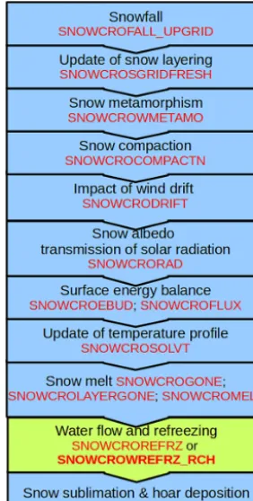
Figure 1.Routines in the Crocus snowpack model with the water percolation routines highlighted in green.
of “most complex snow models” by the Snow Models in-tercomparison project (Etchevers et al., 2004). Crocus is a one-dimensional multilayer model that describes the snow microstructure evolution based on environmental conditions. This model simulates the snowpack from the first snow to melt out, by calculating mass and energy fluxes between snow layers and its interface with the underlying ground and overlying atmosphere. Processes that act on and in the snow-pack are summarized in Vionnet et al. (2012), which are represented in Crocus by routines (shown in Fig. 1). These routines run in a sequential manner. This paper will discuss a new option for the water percolation routine for the Cro-cus model but does not consider aspects of coupling between Crocus and other components in ISBA and SURFEX. For a detailed description of the implementation of Crocus in SURFEX and a detailed description of Crocus see Vionnet et al. (2012).
The SURFEX/ISBA-Crocus default time step is 15 min, denoted as TCrocus, but in this study,TCrocus will be varied
to examine sensitivity. Crocus requires the following forcing variables: air temperature, humidity, wind speed, incoming shortwave and longwave radiation, solid and liquid precipi-tation rate, and atmospheric pressure (Vionnet et al., 2012). Forcing data are generally provided by highly instrumented test sites, output from numerical weather prediction models
(Vernay et al., 2015) or an assimilation or combination of the two (Durand et al., 2009).
The water transport and refreezing processes are expressed in the SNOWCROREFREZ routine (Fig. 1). Feedbacks ex-ist between the liquid water transport (SNOWCROREFREZ) and other processes such as snow compaction (SNOWCRO-COMPACTN) and metamorphism (SNOWCROMETAMO). It is important to realize that changes to the amount and tim-ing of water percolation will feedback to other routines and affect other snowpack variables.
The bucket approach
To describe water percolation in snow, Crocus has histori-cally used an empirihistori-cally based routine, the so-called bucket routine that has been calibrated using long time series of lysimeter data (Morin et al., 2012) and drainage experiments on the irreducible water content (Coleou and Lesaffre, 1998). The bucket routine uses a holding capacity, defined by a percentage of the snow layer pore space. A snow layer’s “bucket” is filled up with water when water is introduced via rain or melt. Once the bucket is full, overflow occurs to fill up the subsequent snow layer’s bucket, restricting water mo-tion in the downward direcmo-tion. The “bucket size” or holding capacity has been defined as 5 % of a layer’s pore spaces as default, although this can be adapted if needed (Vionnet et al., 2012). For Crocus, the holding capacity is proportional to the density of the snow layer but is independent of snow grain type or surrounding environment (adjacent snow lay-ers, soil, etc.). The size of the “buckets” is not agreed upon in the literature, which is discussed in detail in Lafaysse et al. (2017, Sect. 3.7). Singh et al. (1997) found water holding capacity to be 6.8 % of a snow layer’s volume (note this is total volume not just pore space). However, when an imper-meable layer was set beneath it, the holding capacity rose to 14.2 %, showing that the surrounding environment has an ef-fect on LWC of a snow layer, at least for a short time period.
3 Implementation of the Richards routine in Crocus The Richards routine describes motion of water through an unsaturated porous matrix considering capillary-driven and gravity flow. Recent developments in parameterizing the con-ductivity of snow and snowpack water retention allow for the implementation of the Richards equation in layered snow pack models. In contrast to the bucket model, the Richards routine allows for upward motion of water if capillary pres-sure conditions are suitable.
However, Avanzi et al. (2016) found the speed of water trans-port with the Richards equation over a capillary barrier to be underestimated when compared to experimental results, but the model reproduces an increased LWC above barriers.
This paper discusses the implementation of a similar rou-tine in the Crocus model. The new rourou-tine ERCO_RCH represents an alternative to the SNOWCROP-ERCO routine (bucket; Fig. 1). We use the snow layer dis-cretization in Crocus as a mesh for solving the Richards equation.
Richards equation (Eq. 1) is a nonlinear partial differen-tial equation describing the water mass balance of snow with water fluxes expressed using a generalized Darcy law, taking into account the dependence of hydraulic conductivity with water content. Its main variables are the pressure head (h) and the volumetric liquid water content (θ ).
∂θ ∂t =
∂ ∂z
K (θ )·∂H ∂z
(1) K(θ )is the hydraulic conductivity which is a function of the volumetric water content (θ ), andt andzdenote time and depth (positive downward).His the hydraulic head, which is the sum of the pressure head (h) and the elevation (z), which is negative becausezis positive downward (Eq. 2).
H=h−z (2)
The water retention curve and the hydraulic conductivity function need to be expressed for each snow layer.
3.1 Water retention curve
Using the Van Genuchten (1980) parameterization, the water retention curve can be expressed with Eq. (3) if four param-eters (α, n,θr,θs)are known, where α andn are the Van
Genuchten fit parameters (see Eq. 4) and θs (Eq. 5) andθr
(Eq. 7) are the saturated water content and the residual water content, respectively.
θ=θr+(θs−θr)· 1+(α·h)n −1−1n
(3) Recent experiments (Yamaguchi et al., 2010, 2012) and the-oretical estimates based on prior experiments (Daanen and Nieber, 2009) propose parameter sets for these four variables. This paper utilizes the Yamaguchi et al. (2012) parameter set (we also provide options in Crocus to use two alternative pa-rameter sets, see Appendix B).
α=4.4×10⁶·
ρsnow D·1000
−0.98
(4)
n=1+2.7×10³·
ρsnow D·1000
0.61
Here, ρsnowis the dry density of the snow, Dis grain size
diameter andP is porosity (volume of pore space).
θs=0.9×P (5)
Yamaguchi et al. (2012) performed a drainage experiment to obtain the Van Genuchten fit parameters. The gravita-tional drainage experiment assumed the saturated hydraulic conductivity θs for snow to be 90 % of the pore spaces.
This is due to small air bubbles that become trapped in the pores between the snow grains as the snow saturates. One should note that Yamaguchi’s study examined samples of melt form and small rounded grains with a density range of 361–636 kg m−3and grain size range of 0.05 to 5.8 mm. Columns of snow were saturated with 0◦C water and left to drain. The study found a parameter set for melt-form crystals and concluded that rounded crystals could not be represented with the same parameter set as melt forms.
The Van Genuchten parameterization being applied is adopted from soil science for flow in an unsaturated soil ma-trix. The residual water content in snow presents specific challenges that are not present when applied to soil. Snow is often completely dry via phase transform, whereas soil is assumed to always have a small amount of liquid water. The termθris defined as the amount of water that remains in the
porous medium with infinite suction being applied. It corre-sponds to disconnected water patches entrapped in the pore system. Following Yamaguchi et al. (2010), a residual water contentθr=0.02 is adopted. However, the LWC of a snow
sample can further “dry out” via evaporation and freezing, resulting in a negative saturation. (S)
S= θ−θr θs−θr
, whereθr< θ < θs (6)
Negative saturation (where 0≤θ < θr)is physically possible
with phase change, but causes numerical problems. There-fore, saturation needs to be restricted between 0 and 1. To overcome this limitation we use a continuous piecewise func-tion to keepθ > θr.
θr=
0.02 if θ >0.02
0.75·θ if θ≤0.02 (7)
To avoid infinite values of the hydraulic head (Fig. 2) and hy-draulic conductivity (Fig. 3, Sect. 3.2) of 0 when approaching LWC=0, a small amount of water needs to be added to snow layers that are completely dry. Water is added to the dry lay-ers such that all dry laylay-ers start with the same pressure head, which corresponds to a minimum pressure head needed to keep all dry layers≤θmin. In this study we call this added
water “prewetting”. The default value ofθmin=10−5
(unit-less) was adopted, although a sensitivity test varies the value ofθmin.
3.2 Hydraulic conductivity
Hydraulic conductivity (K) is a function of water content (θ ); see Eq. (8). As a snow layer gets wetter the conductivity will increase (Fig. 3).
Figure 2.Water retention curve using Yamaguchi et al. (2012) in the Van Genuchten (1980) parameterization. Typical values for density and grain sizes of different snow crystals or grains were chosen to show hydraulic head as a function of saturation for different snow layers that it is applied to in the Richards routine. The density and grain size values were chosen from each crystal type from within a reasonable range that may be found in nature. Background shows a histogram of the simulated data sets’ saturation with aTCrocus=
900 s time step before entering the Richards routine (leftyaxis).
Figure 3. Hydraulic conductivity curve derived from Calonne et al. (2012) using Yamaguchi et al. (2012) parameters. Typical val-ues for density and grain sizes of different snow crystals or grains were chosen to show the hydraulic conductivity for the spectrum of different snow layers that it is applied to in the Richards routine. The density and grain size values were chosen from each crystal type from within a reasonable range that may be found in nature. Background shows a histogram of the simulated data sets’ satura-tion with aTCrocus=900 s time step before entering the Richards
routine (leftyaxis).
The Van Genuchten–Mualem equation (Van Genuchten, 1980 and Eq. 9) is used to calculate the relative permeability kr. It is implemented as a function ofh(using Eq. 3 for the
relation betweenhandθ ):
kr=
1+ |α·h|1−1m −2m
(9)
·
1−
1−1+ |α·h|1−1m
−1m2
wherem=1−1/n. Hydraulic conductivity reaches a max-imum when the snow matrix is saturated, known as conduc-tivity at saturation (Ksat). Since conductivity at saturation is
dictated by snow structure, which is a complex system, it is described by a simple statistical model in both parameter sets available. It should be noted that bothKsat (Eq. 10) andkr
(Eq. 9 throughαandm) are dependent on the dry density of the snow and the grain size.
Calonne et al. (2012) used three-dimensional images of the microstructure of snow to derive the permeability (con-ductivity) from different snow types and densities ranging from<100 kg m−3to∼550 kg m−3, seen in Eq. (10). Equa-tion (10) is the preferred parameter set due to the range of snow types and densities that went into deriving the equation (other alternatives are described in Appendix B).
Ksat=3.0·
D
2 2
·exp(−0.013·ρsnow)· G·ρ
water µwater
(10)
G=9.816 m s−2 is the acceleration due to gravity, and µwater=0.001792 kg m−1s−1 is the dynamic viscosity of
water at 0◦C.
3.3 Solving the Richards equation
To reduce unnecessary computations, the following two con-ditions need to be satisfied before entering the Richards rou-tine.
1. There must be a substantial snowpack: if there are fewer than three layers of snow the bucket model will be used for water percolation.
2. There must liquid water:θ < θmin, or the rain flux (over
the time step of 15 min)<10−10m.
If one of these two conditions are not satisfied Crocus will be run without calling the Richards routine.
To solve the Richards equation, we utilize the following strategy: a finite volume discretization is applied taking each snow layer as integration volume. The average pressure head of each snow layer (corresponding to its LWC) is supposed to apply in the center of the layer.
the flux at the top and the bottom are computed respectively as follows:
8ti,+1top=Ktopt+1
θit+1, θit−1+1 ht+1
i−1−h
t+1 i 1ztop +1 ! , (11)
8ti,+1bot=Kbott+1θi,t+1, θit+1+1 h t+1
i+1−h
t+1 i 1zbot −1 ! ,
where i is the index for snow layer (layer 1 at top of the snow pack). Values on the interface between two snow layers are indicated with “top” and “bot” (bottom) subscript respec-tively.
Ktop and Kbot are the hydraulic conductivity of the
up-per and lower boundary interfaces of layeri, respectively. To compute KtopandKbotthe arithmetic mean was used as an
estimate of the conductivity at snow layer interfaces, shown in Eq. (12).
Ktop=
Ki·1zi+Ki−1·1zi−1 1zi+1zi−1
(12) Kbot=
Ki·1zi+Ki+1·1zi+1 1zi+1zi+1
The terms 1zbot and1ztopare the distance between layer
mid-points, as described below in Eq. (13). 1ztop=
1zi+1zi−1
2 1zbot=
1zi+1zi+1
2 (13)
Averaging conductivity of two adjacent snow layers with a simple arithmetic mean as an estimate for the interface value may be over-simplifying the conductivity of snow. Snow grain size, density and crystal types often have sharply de-fined borders. These parameters would have great influence on the snow hydraulic conductivity. It could be argued that a piecewise function comprised of individual snow layers’ conductivity better describes the vertical pattern of conduc-tivity in the snow pack (Szymkiewicz, 2009). However, when a piecewise function was tested, “dry layers” (that needed prewetting) caused impermeable barriers and caused numeri-cal problems for the simulation. Other options for combining conductivity values of snow layers to estimate the interface are possible, but more research is needed to understand how the interface conductivity behaves.
The time discretization is a Crank–Nicolson finite differ-ences scheme, which is second-order accurate in time. The nonlinearity of the equation is then dealt with the iterative methodology proposed by Celia et al. (1990). It approximates θit+1,k+1by a truncated Taylor series:
θit+1,k+1=θit+1,k+ dθ
dh
t+1,k i
hti+1,k+1−hti+1,k, (14) where the superscriptkrefers to the evolution of the iterative process, and ddθh
t+1,k
i is the derivative of the retention curve
(Eq. 3) computed analytically forθit+1,k(orhti+1,k). The final discretized form of the Richards equation (Eq. 1) including the Crank–Nicolson scheme with Celia decomposition reads as follows:
θit+1,k+Cht+1,khit+1,k+1−hti+1,k−θit
1t 1zi (15)
=0.58ti,+1top,k+1+8i,t+1bot,k+1+0.58ti,top+8ti,bot.
The system of discretized equations is solved with respect to the pressure head h at iteration level k+1. The three-diagonal linear system is solved with the direct LU Thomas algorithm. The value of the volumetric content is then up-dated until the convergence criterion of the Picard iterative process is reached (see Appendix A).
The Richards equation is solved on a variable time step de-noted with a1t(see Appendix A for how time step varies). The SURFEX/Crocus model is run on a fixed time step TCrocus, which is set to 15 min unless otherwise specified.
Snow layer properties such as grain size and snow density and snow layer temperature are updated on eachTCrocus. The
variable time step segmentsTCrocus up into smaller steps as
needed, until61t=TCrocus. Outflow to soil and liquid water
content of each layer are updated in the main Crocus routine when the time steps join. Finally, density, snow temperature and liquid water content are updated and the Crocus routine is finished.
3.4 Boundary conditions
The rain rate and evaporation rate are imposed as a flux for the upper boundary condition. For the snow–atmosphere interface, rain and evaporation rates replace 8ti,+1top,k+1 and 8ti,top. Both rain and evaporation fluxes are provided from the meteorological forcing.
The lower boundary is the soil snow interface. There are two options for the bottom boundary: one uses soil properties from the ISBA soil routine, the other is a free-flowing bottom boundary.
3.4.1 Bottom boundary with soil properties
Properties from the upper-most soil layer are imported from the Surfex/ISBA soil routine, which also uses the Richards equation for unsaturated water flow. Interfacial conductivity between the soil and bottom snow layer Kbot is calculated
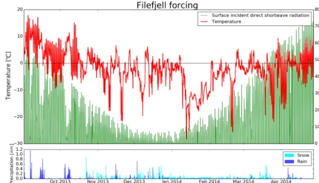
Figure 4.Forcing data from an automatic weather station located at Filefjell, Norway, for the period 1 September 2013 to 31 May 2014.
3.4.2 Free-flow bottom boundary
A free-flowing bottom boundary has been added where the pressure gradient of the last two snow layers is applied at the bottom boundary. The hydraulic conductivity of the last snow layers is used at the snow–soil interface. Water cannot move from the soil to the snowpack. If the pressure gradient of the bottom two snow layers is upward, the pressure at the snow– soil interface is set to 0 m. All plots shown in this paper use the free-flowing boundary.
4 Forcing data and experiments
The Richards routine was tested on two data sets: one is from Filefjell, Norway (61.178231◦N, 8.112925◦E), recorded at an automatic weather station by the Norwegian Water and Energy Directorate (NVE), and the other is a synthetic data set.
4.1 Filefjell
The Filefjell data set was recorded at hourly steps over the 2013–2014 winter at a flat field at 956 m a.s.l. Filefjell is lo-cated about 200 km northwest of Oslo. Despite being 30 km inland from the end of a fjord, Filefjell is considered to have a continental snow climate, which has an average precipita-tion of 603 mm yr−1and large annual temperature variation, shown in Fig. 4. Continental snow climates are characterized by thin snow covers, cold temperatures and few rain-on-snow events during the winter months (McClung and Schaerer, 2006). Air temperatures become as cold as −28.3◦C, and after January there is a long cold spell during which tem-peratures stay well below zero for about a month. The sur-face incident shortwave radiation is low during winter, when maximum daily values are below 300 W m−2from 18 Octo-ber 2013 to 19 February 2014, due to the high latitude. The
first large rain-on-snow event occurs on 7 March 2013, with a second event on 6 and 7 April 2013. Early winter rain-on-snow events occurred before January, which is not typical for continental climates. Unfortunately, no manual snow pit measurements at the field site have been conducted during the winter of 2013–2014.
4.2 Synthetic
Figure 5 shows the 90-day synthetic data set. The peak short-wave radiation values for this data set are low and increase linearly from 100 to 200 W m−2. Temperature has a linear increase from 265 to 276 K. The temperature and radiation patterns set in the synthetic data set were chosen to induce a modest melt rate early in the simulation that is ramped up to a heavy melt rate at the end of the simulation. The syn-thetic data set is designed to test the new routines for a large range of water supply rates. This data set has two large snow events: the first one starts on day 3 and deposits 2.6 m over 5 days, and the second event occurs on day 60 after the first snow event had a chance to settle down to 1.1 m and the di-urnal radiation cycle had formed a melt freeze crust at the surface. The second snowfall buried the old surface crust un-der 1.8 m of snow (for Richards routing, 1.9 for bucket rou-tine). The second snowfall was deposited with density varia-tions, an effect of the radiation cycle. The synthetic data set allows for a simple comparison between the Richards routine and bucket routine without complicated snowpack structures, over a wide variety of melt intensities.
4.3 SURFEX configuration of the model runs
spheric-Figure 5.Simulated forcing data. Temperature (red) and net radiation (green) both linearly increase, creating low melt early in the simulation and high melt at the end of the data set.
ity to describe the microstructure of snow. The free-flowing boundary was used for the bottom boundary condition in the Richards routine. The default time step (TCrocus)was used
unless otherwise specified. Every 900 s the prognostic and diagnostic variables were saved despite duration ofTCrocsu.
5 Results
5.1 Filefjell Simulation
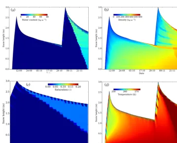
Simulation results for the Filefjell data set are presented in Fig. 6, with the top (Fig. 6a and b) showing the amount of liquid water and snow layer density from the simulation run with the bucket routine and the bottom (Fig. 6c and d) with the Richards routine. The snowpack thickness reaches just over 1 m (1.1 m for the Richards routine and 1.2 m for the bucket routine) at its maximum in March before a fast melt out. The difference in snow thickness between the two rou-tines is due to the wet-snow compaction that relies on the LWC. The majority of the snowpack wetting occurs during the April melt. The wetting front reaches the bottom of the snowpack at approximately the same time independent of which routine was used (Fig. 6a and c). The three rain and melt events that occur early in the season (23–24 October, 15 and 26 November) pass water to the soil layers for both per-colation routines. The two melt and rain events that occur af-ter the cold period in January (7 March and 6–7 April) cause the surface layers to get wet, while deeper layers remain be-low freezing. These two events are more pronounced and reach deeper snow layers in the simulation using the Richards routine. The event on 7 March formed a layer with density
∼300 kg m−3(at 0.7 to 0.9 m) when run with the Richards routine, which is missing from simulations using the bucket routine (see Fig. 6b and d).
The density evolution according to the bucket routine (Fig. 6b) shows the formation of a dense crust at the bottom of the snowpack of about 375 kg m−3, where the Richards routine (Fig. 6d) creates a much thicker and denser layer of >600 kg m−3. The Richards routine makes a slightly denser preisothermal snowpack and a much denser snowpack dur-ing periods of enhanced water transport. The bucket routine allows easy transmission through crust layers because high-density layers yield low pore volumes resulting in a “small bucket size”. The bucket routine does not represent crust lay-ers well because they develop to be too thick and not dense enough.
5.2 Synthetic data set’s simulation
Figure 6.Crocus output from Filefjell, Norway, in which the top plots use the bucket routine and the bottom plots use the Richards routine. Panels(a, c)show distribution of liquid water, and(b, d)show the density distribution.Tcrocus=900 s (15 min) was the time step duration.
Figure 7.Crocus output for simulated forcing using the bucket routine withTCrocus=900 s (15 min), plotted every 3 h, except for(c), which
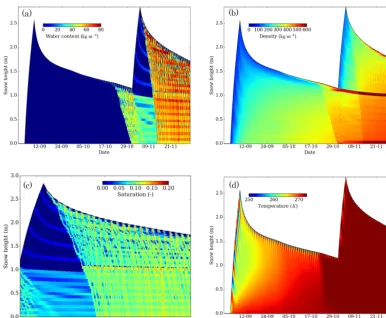
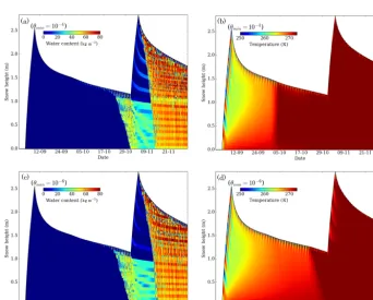
Figure 8.Crocus output for simulated forcing using the Richards routine withTCrocus=900 s (15 min). The bottom boundary is set to free flow, withθmin=10−5.(a)Liquid water amount,(b)snow layer density,(c)percentage of pore volume filled with water zoomed in on the
second snow event and(d)temperature development of the snowpack.
A pattern emerges after meltwater from after the second snow event reaches the bottom snow layer Fig. 8a where yel-low and red stripes appear (also seen in Figs. 6c and 8c, al-beit less pronounced). Every second snow layer remains very wet with 10–12 % pore volume corresponding to a water con-tent of 60–80 kg m−3. Figure 8c shows interesting behavior of many newly wet-snow layers quickly draining to less than 5 % saturation after the water front has percolated to deeper layers.
The bucket routine run with the synthetic forcing (Fig. 7b), produces a thick crust layer that does not exceed a density of about 400 kg m−3. There is no delay in the water front’s movement as it passes the melt freeze crust in Fig. 7b. The Richards routine produces a melt freeze crust that is thicker and more dense (about 500 kg m−2)than the bucket routine.
5.3 Sensitivity of prewetting and time step
The temperature development of the snowpack for both the Richards and bucket routines lead the wetting front. How-ever, changing the length ofTCrocus(Fig. 9) will change the
timing of the warming and water front. When TCrocus is
re-duced the warming and wetting front is able to percolate much faster.
Ifθminis larger than 10−5 the temperature of the
snow-pack would become isothermal long before the wetting front. Ifθminis kept below 10−5the temperature and water
distri-bution are not changed significantly. Appendix A discusses a sensitivity test on the prewetting amount and how the default θminwas set.
5.4 Feedback from compaction and metamorphism routines
Figure 9.Crocus output for simulated forcing showing different time steps:(a)TCrocus=900 s (15 min),(b)TCrocus=60 s both plots use
the free-flowing bottom boundary with prewetting set toθmin=10−5. The 60 s simulation has water at the bottom of the snowpack 4 days
before the 900 s simulation.
Figure 10.Crocus output for simulated forcing with SNOWCROMETAMO (snow metamorphism routine) and SNOWCROCOMPACT (snow compaction routine) turned off. The time stept was restricted to maximum of 30 s for numerical stability. Panel(a)shows water content (kg m−3) and(b)is the saturation (unitless); these plots show that without feedback the Richards routine percolates water down the snowpack with maximum LWC<10 %.
which keeps snow layers moderately wet and firmly in the pendular regime. The bucket routine is much less dynamic in regard to fluctuations of water content. The alternating horizontal stripes (yellow, red pattern in Fig. 8a) in wa-ter content apparently are influenced by snow properties, as demonstrated in a numerical experiment in which snow metamorphism (SNOWCROMETAMO) and compaction (SNOWCROCOMPACTN) routines have been disabled, re-sulting in the disappearance of these stripes (Fig. 10). How-ever, Fig. 10 should be interpreted with care because turning off SNOWCROMETAMO and/or SNOWCROCOMPACTN results in unphysical snowpack conditions, beyond the do-main for which the parameterizations have been originally designed for.
6 Discussion
Comparing Figs. 7a and 8a shows that the Richards rou-tine creates an isothermal snowpack and water percolation to deep layers earlier in the simulation than the bucket routine. However, the propagation of the warming and water fronts depends on many variables. The following sections discuss some of the parameters that we found to have influence over the timing and amount of water flow and some of the limita-tions and assumplimita-tions used in the routine.
output saving may further contribute to increase the differ-ence in computational cost.
6.1 Liquid water content magnitude
The bucket routine has a LWC upper limit of 5 % pore space. There are two wetness states that are frequented in the bucket routine, the dry state and wet state at holding capacity. A snow layer spends little time over the course of a snow season in the transition between dry and at holding capacity, which can be seen in Figs. 6b and 7c. Routines such as the com-paction and grain metamorphism were developed using the bucket routine and rely on a nearly binary water content con-figuration.
Using the Richards routine, we obtain much higher LWCs, which constantly vary between time steps (Figs. 6c and 8a). The Richards routine is capable of wetting snow layers to the transition between pendular and funicular regimes, as defined by Denoth (1980), in which 18 % of the simulated data sets’ snow layers that entered the percolation routine had>10 % of their pores filled with water. This study did not investi-gate how other routines in Crocus (e.g., the compaction rou-tine) that are affected by the LWC are affected by high LWCs in snow layers. However, it is expected that wet-snow com-paction and wet grain metamorphism are nonlinear functions with feedback on LWC in the transition between pendular and funicular, since the physical distribution of water is held differently in the snow’s pores with respect to snow crystal surfaces (Denoth, 1982).
6.2 Bottom boundary
The bottom boundary is an area of concern because it feeds the soil water percolation routine with meltwater, and differ-ences in pore structure over the snow–soil interface will often create a textural barrier, which can lead to pooling or acceler-ated flow. The advantage of running the Crocus model cou-pled with SURFEX and ISBA is that the boundaries of the Crocus model (atmosphere and soil) are better represented and dynamic. The free-flowing boundary does not take ad-vantage of the coupling between Crocus and ISBA, but shows better results in the current organization of SURFEX, ISBA and Crocus. We recognize the bottom boundary as a part of the routine that needs more development, so that the Richards routine can take full advantage of SURFEX and ISBA. 6.2.1 Bottom boundary with soil properties
The performance of the bottom boundary when soil condi-tions are used is not satisfactory. The flux to the soil remains lower than when the free-flowing boundary is used. This re-sults (not shown) in higher saturations of all snow layers af-ter the bottom snow layer becomes wet. The higher LWCs increase the feedback from other crocus routines, thus en-hancing the “yellow/red striped pattern” (seen in Fig. 8a).
When using the upper soil layer as lower boundary for the snowpack, the hydraulic conductivity of the bottom soil layer and the suction of the soil layer are imported to Cro-cus from the soil routine. These values are held fixed for the time stepTCrocus. The hydraulic conductivity of the
bot-tom interface is the arithmetic mean (harmonic mean can be used) of the bottom snow layer and the top soil layer’s thickness and hydraulic conductivity. Snow layers are able to move water between them on the internal time step (t), which can be as small as a fraction of a second. Snow layer suc-tion and conductivity are altered on the internal time step (t). However, the soil suction and conductivity remains constant until6t=TCrocuswhich means the snow–soil interface has
less-dynamic conductivity and suction because half the val-ues making up theKsnow−−soil are constant onTcrocus. One
way to force the bottom interface to be more dynamic is to reduceTCrocus (Sect. 5.3). A second way is to increase the
top soil layers’ thickness, in which case the snow layer will dominate in the weighted average used for conductivity at the snow–soil interface. However, increasing the size of the soil reduces the reliability of the snow–soil thermodynamics routine, but that is beyond the scope of this study.
Ideally, the snowpack and soil column would be solved as one continuous column (Wever et al., 2014). However, the snowpack is semiimplicitly coupled to the soil percolation routine onTCrocus. Unfortunately, with the ISBA model the
soil and snow routines are not coupled on the variable time stept. To solve the soil and snow as one continuous column of unsaturated porous media would take major reorganizing of the SURFEX model and was not feasible during this study, but should be considered in the future.
6.2.2 Free-flow bottom boundary
6.3 Coupling
TCrocus dictates the degree of coupling between SURFEX
routines, including the coupling between the ISBA and Cro-cus and between routines in CroCro-cus. The water percolation process is coupled to the soil percolation process and the energy balance of the snowpack; in Crocus these routines are run sequentially and are coupled viaTCrocus. The energy
balance is made up of many processes that are expressed through many of the routines in Crocus (see Fig. 1). The tem-perature of the snow layers is altered after the percolation routines (for both Richards and bucket) due to latent heat re-lease, if refreezing occurs. Although a sensitivity study on the link between temperature of snow layers and percolation would be relevant, such a study was not possible because of other feedbacks in the model.
The histograms in Figs. 2 and 3 show the distribution of snow layer saturation upon entry to the Richards routine. The water content is often very low, with 49.5 % of the snow lay-ers under 5 % LWC for the simulated data set. At low sat-urations, the hydraulic conductivity function and the reten-tion curve are very sensitive to changes in density, grain size and saturation. It is important to note that a 1 % change in saturation when very dry can affect both the hydraulic con-ductivity and the water retention curves by orders of mag-nitude. Figure 9 shows the simulated forcing when run with TCrocus=900 s andTCrocus=60 s. Water moves through the
snowpack earlier when TCrocus=60 s because feedback
be-tween the percolation routine and routines that alter layer density and layer grain size are more effective and faster act-ing.
6.4 Feedback from compaction and metamorphism routines
There are two major differences between the Richards rou-tine and the bucket model concerning the behavior of the water content within a snow layer. The bucket routine keeps water saturation at moderate levels, with very little fluctu-ation in saturfluctu-ation once the holding capacity is reached. In contrast, saturation of up to 90 % of the pore space can be reached with the Richards routine (however, our saturations never reached>20 % with the simulated forcing), with con-stant small (<1 %) fluctuations in the saturation over the du-ration of the simulation. The cause of the striped pattern (in Fig. 8a) has been identified as stemming from an incomplete description of wet-snow metamorphism and compaction in the routines SNOWCROMETAMO and SNOWCROCOM-PACTN (Fig. 1) which have been developed for use with the bucket routine. There is significant feedback between the Richards routine and the metamorphism and compaction rou-tines in Crocus as the parameterizations used are heavily re-liant on snow grain size and snow density. Figure 10 shows that the Richards routine is numerically stable, when run
without feedback from the metamorphism and compaction routines, and does not produce the striped pattern.
Examining how an increase in grain size (or density) will affect the water retention curve and hydraulic conduc-tivity with Figs. 2 and 3 highlights the complexity of the feedback system. Comparing the water retention curve for small rounds (400 kg m−3, 0.5 mm diameter) with that of melt forms of identical density (400 kg m−3, 1 mm diame-ter, Fig. 2) shows that the response of the water retention curve to an increase in snow grain size depends on the uration of the snow layer. For instance, at low levels of sat-uration (<0.2), a smaller grain size is associated with lower hydraulic head, but this is reversed at higher saturation levels at which smaller grains will induce a higher head. A similar grain size dependency is also observed for the hydraulic con-ductivity (Fig. 3). This means that as grains grow, the suction or hydraulic conductivity may increase or decrease depend-ing on the saturation. Similar behavior holds for changdepend-ing the density at a fixed grain size. This indicates that snow meta-morphism can induce alternating gradients in hydraulic snow properties, eventually leading to the observed “striped pat-tern”. This behavior appears nonplausible but the validity of the water retention curve and hydraulic conductivity param-eterizations for the wet-snow regime needs to be established in future work before this issue can be resolved.
6.5 Conductivity through crusts
The Richards routine is able to produce crust layers from meltwater that the bucket routine cannot reproduce, like the melt freeze crust in Fig. 8b. However, the thickness and den-sity of crust layers depend on where the percolation routine moves water, since refrozen liquid water is often the cause of crusts at the surface and inside the snowpack. The water retention curve and hydraulic conductivity functions are not designed for use on crust layers. Furthermore, Crocus’ snow metamorphism routine (SNOWCROMETAMO, Fig. 1) does not work well for crust layers, because dense crusts do not have individual grains, but rather a solid ice layer with bub-bles. There is a choice of routines in SNOWCROMETAMO, the B92 and the C13 routines. The B92 routine uses spheric-ity and dendricspheric-ity. The C13 routine uses optical diameter, which is used as an approximation for visual grain size in the Richards routine. The assumption that optical diameter is a sound approximation for visual grain size is questionable, especially for crust layers. Nevertheless the metamorphism routine calculates a grain size for all layers including crusts (see Sect. 6.6). Figure 8b shows that the crust layer was able to develop into a thinner and denser crust compared with the bucket routine Fig. 7b. Since there is no literature available on water retention and hydraulic conductivity of crust layers, crusts are treated like normal snow layers in both percolation routines.
have shown that water transport though snow is a three-dimensional process (Williams et al., 2010). When the wet-ting front reaches a barrier such as a crust or capillary dif-ferences, the underlying snow layer will probably develop flow channels where a one-dimensional model does not suf-fice. Averaging the hydraulic conductivity between a layer’s barrier suction with the flow channel suction is one way to express a three-dimensional process in one dimension. Hy-draulic conductivity has been determined (via permittivity) by Calonne et al. (2012) on small snow samples, and there-fore it is likely that the measurements do not represent con-ductivity on a higher spatial scale because processes that af-fect the density distribution, grain metamorphism and pore space differ on scales of a meter to several meters (Birkeland et al., 1995).
6.6 Grain metamorphism routine
The hydraulic conductivity function derived from Calonne et al. (2012) utilizes the optical grain diameter and snow den-sity. The hydraulic conductivity function pairs well with the C13 routine, because they both use optical grain diameter. However, the water retention curve (Yamaguchi et al., 2012) was based on visual grain size measurements and the use of optical grain diameter may hinder the performance of the wa-ter retention curve.
The pore shape and structure is important for the retention curve and the hydraulic conductivity. Small pores inside the snow layer create suction via capillary rise, and water travels through the voids in the snowpack. Both parameterizations could benefit from a better description of the pores’ struc-ture. Density and grain size is not enough to describe the pore structure of a snow sample. We use optical diameter for parametrization, but in nature optical properties do not influ-ence the hydrological processes of snow. For the retention curve and the conductivity functions to be used at low satu-rations, pore shape and structure should be considered. Intro-ducing a routine in Crocus that calculates pore shape could be beneficial for not only the water percolation routine but also the thermal conductivity (Riche and Schneebeli, 2013; Sturm et al., 1997). This would also require new parameteri-zations including a pore structure variable with the grain size and density.
6.7 Water retention curve
The Yamaguchi et al. (2012) water retention curve has been applied to melt-form crystal types and reported poor perfor-mance with rounded grains. It is expected that the retention curve does not represent precipitation particles, decomposing and fragmented precipitation particles, faceted crystals and depth hoar well. However, when water is present in a snow layer, snow grain metamorphism will transform all snow crystals into melt forms (Colbeck, 1976; Shimizu, 1970). This negative feedback on snow grain type could mean the
melt forms are the only crystals that need to be described by a water retention curve, but this claim needs validation.
The residual water content is one of four parameters needed to define the water retention curve. The residual wa-ter content represents how dry a layer can get with maxi-mum suction applied. A constantθr was used for different
grain types, sizes and densities but results from Adachi et al. (2012) and Leroux and Pomeroy (2017) suggest thatθr
varies with grain size.
Hysteresis in the water retention curve stems from oddly shaped pores, which mean that pores can hold different amounts of water at the same hydraulic head depending on the initial LWC. In most cases, snow will go from a dry state (pore space filled completely with air) and become wet. The Yamaguchi parameters for the van Genuchten model are derived from a drainage experiment, in which the pore space was completely filled with water and allowed to drain. Adachi et al. (2012) showed that the shape of the water reten-tion curve is affected more in fine-textured grains than coarse grains.
Parametrization of the water retention curve based on a wider range of snow grain types and sizes are needed to rep-resent natural snow pack conditions. For fine-textured snow, parameter sets derived from wetting experiments would be beneficial, as the snow usually starts from a dry state.
7 Conclusion
A water percolation routine that solves the Richards equa-tion was added to the Crocus model as a physically based alternative to the empirical bucket routine. However, the per-formance of the Richards routine is not sufficient for simu-lations of the snowpack, because further work is needed on other parts of the Crocus model that feedback on the param-eter sets used by the Richards routine.
The bucket model keeps snow layers in the pendular wetness regime. The Richards routine reaches LWCs much higher than the bucket routine, with water filling>17 % pore volume for many snow layers, which lies in the funicular regime for all snow types. However, 18 % of snow layers entered the Richards routine with<10 % of the pore space filled with water (bucket routine has max 5 %). With small changes in LWC at low saturation, the suction and hydraulic conductivity can change by orders of magnitude.
reten-tion curve that do not contain grain size are needed for dense crust layers. The Richards routine in the current state treats crusts as a normal snow layer in which grain size calculations are erroneous. The parameterization for the water retention curve was based on a small domain of densities, grain sizes and snow types. In the future, the domain for this parameter set should be expanded for applicability in snow grains other than melt forms. New parameter sets should be based on wet-ting experiments for small grain sizes as hysteresis affects the Van Genuchten parameters (θr,α,n).
The snow–soil interface does not perform well during pe-riods in which large amounts of meltwater should pass from the snowpack to the soil. Soil parameters (suction and hy-draulic conductivity) are updated on a 15 min time step, which is not fast enough during periods of high water flux. At the current state of the Crocus model, major structural changes are needed in order to couple the soil and snow on the variable time step used by the Richards routine. A free-flowing bottom boundary shows better results during high flux periods but does not take advantage of the ability to run Crocus in SURFEX coupled with ISBA.
Because of the number of areas of concern in the valid-ity of the Richards routine, we did not attempt a validation experiment. In order to further develop the Richards rou-tine, improvements and updates are needed in other Crocus routines (mostly melt, compaction and grain metamorphism) and/or the parameter sets used by the Richards routine, which is beyond the scope of this study.
Code and data availability. For directions and help with down-loading, compiling and running the code you will need to register as a user at https://opensource.umr-cnrm.fr/. The SUR-FEX/CrocusV7 with the Richards routine can be downloaded via Git by following instructions at https://opensource.umr-cnrm.fr/ projects/snowtools/wiki/Install_SURFEX and downloading the branch “damboise_dev” with the “damboise_et_al.2017” tag. Directions for running SURFEX (with Crocus) can be found here: https://opensource.umrcnrm.fr/projects/snowtools/wiki/ Basic_functioning_of_SURFEX_without_the_s2m_tool_from_ snowtools. The Wiki can be a useful resource for troubleshooting https://opensource.umrcnrm.fr/projects/snowtools/wiki/Wiki.
Appendix A: Picard iteration and convergence
A Picard iteration is used to deal with the nonlinear nature of the system of equations. There are three convergence tests that need to be satisfied to calculate the next internal time step (t). The three convergence criteria are on pressure head dif-ferences, volumetric water content differences and the mass balance (of individual snow layers) differences between two iterations and must be below 10−4m. Hence, there must be at least two iterations performed in order to test for conver-gence. If the current iterations’ deviations of pressure, volu-metric water content and mass balance are smaller than the error threshold that has been set, then the convergence crite-ria are met and the model proceeds to the next time step. The threshold of 10−4m is a large amount of water considering it can be added at every time stept. However, the simulated data set has a maximum mass balance of 0.0011 kg m−1s−1 over the full domain overTcrocus(15 min). The 15 min mass
balance over the full domain is acceptable, when consider-ing the synthetic data set was made to test extreme wettconsider-ing and drying cycles, and snow layers often reach LWC>10 % which is seldom the case in nature. Addressing the feedback issues described in Sects. 5.4 and 6.4 should reduce the num-ber of layers at a high LWC and duration layers remain at high LWC.
A set of rules are used to regulate the variable time step based on the number of iterations needed for convergence, similar to Paniconi and Putti (1994). A maximum number of iterations has been set to 15. If the calculations do not converge by the 15th iteration then the time step is reduced and calculations are preformed again, until the calculations converge within 15 time steps. The variable time step can range in time from about 400 s to fractions of a second within a lower limit of 1×10⁻¹⁰s. Smaller time steps within the Richards routine result in the model taking too long to run or convergence not being achieved. If convergence is reached in 4–7 iterations the time step is kept constant. Converging in less than 4 or between 8 and 15 iterations results in a longer or shorter time step, respectively (Eq. A1).
ti+1=
ti·1.5BS, I <4 ti, 4≤I <7 ti·0.5SS, 7≤I <15 back step, 15< I
(A1)
Here,I is the number of iterations and “back step” stops the calculation before convergence and reduces the ti. BS and SS are initialized at 1 and is increased by 1 for the previous “bigger steps” or “smaller steps”. BS and SS are reinitialized if the time step remains the same size (4≤I <7).
Appendix B: Alternative parameter sets
The following sections describe alternative parameter sets for hydraulic conductivity (Sect. B1) and water retention curve
(Sect. B2, B3) that we implemented in the Richards routine, but is not presented in this paper.
B1 Shimizu (1970)
Shimizu developed a statistical model forksatfrom the
den-sity and grain size of fine-grained compact snow, Eq. (B1). Shimizu suggests that other snow grain types and densities may give different coefficients to those found in Eq. (B1). For use in the Richards routine this parameter set would have to be applied to lower density snow than that used to create it.
Equation (B1) relates snow density and grain size to con-ductivity at saturation (ksat).
ksat=0.077·
D
2 2
·exp(−0.078·ρsnow) (B1) ·
G·ρ water µwater
B2 Yamaguchi et al. (2010)
This parameter set was the prior work of the parameter set used in this study. Two major differences (when compared with Yamaguchi et al., 2012) for this parameter set areαand n, which are functions of grain diameter (D) and not den-sity. The density range used in the Yamaguchi et al. (2010) parameterization is small, 545–553 kg m−3. The parameter-ization for the θr andθs are the same as in Yamaguchi et
al. (2012).
α=7.3·(D·1000)+1.90 (B2)
n=15.68·exp(D·1000)·(−0.46)+1.00 B3 Daanen and Nieber (2009)
Daanen and Nieber derived these relations based on mea-surements of liquid water content and water pressure from Marsh (1991)hey assume snow crystals to be between 1 and 0.1 mm. However, descriptions of the measurements are not given in detail. The Daanen and Nieber study focuses on a framework of a coupled temperature and liquid water routine that does not focus on deriving the Van Genuchten fit param-eters in a suitable way for different snow types, as all crystals are assumed to be spheres.
α=30·(D·1000)+12.00 (B3)
n=0.8·(D·1000)+3.00 θr=0.05
Appendix C: Prewetting
In order to apply the Richards equation in snow the Van Genuchten parameterization needs snow layers to have a small amount of liquid water. The amount of “prewetting”, is set byθmin. A sensitivity study was done onθminbecause
the parameter is not physical but necessary for numerical sta-bility. The results showed that the temperature, density and liquid water content of the snow layers were not sensitive when θmin≤10−5. The temperature evolution of the snow
pack is drastically different whenθmin>10−5, although the
timing of the percolation front and the distribution of wa-ter in the snowpack is not affected much. When too much water is used for prewetting, the snowpack becomes isother-mal when the surface becomes wet (Fig. C1). Therefore the default value ofθmin=10−5was chosen. Figure C1 shows
how the temperature evolution is affected by the magnitude of θmin. Ifθminis too large the snow pack becomes
isother-mal quickly after the top snow layer becomes wet for the first time. However ifθminis too low the simulation may not
con-verge, or the simulation takes much longer to run because of the extreme pressure difference between wet and dry layers.
Figure C1. Water percolation and temperature evolution in the simulated data set with different prewetting amounts; plots use the free-flowing bottom boundary with prewetting set toθmin=10−4 for(a)water content and(b)temperature andθmin=10−6 for(c)water
Competing interests. The authors declare that they have no conflict of interest.
Acknowledgements. We thank the NIFS project (www.naturfare. no) for the financial support of this study. We would like to thank Nander Wever and one anonymous referee for the useful comments which improved the quality of this paper. IGE and CNRM/CEN are part of LabEX OSUG@2020.
Edited by: Jeremy Fyke
Reviewed by: Nander Wever and one anonymous referee
References
Adachia, S., Yamaguchia, S., Ozekib, T., and Kosec, K.: Hystere-sis in the water retention curve of snow measured using an MRI system, available at: http://arc.lib.montana.edu/snow-science/ objects/issw-2012-918-922.pdf (last access: 6 July 2016), 2012. Ambach, W. and Howorka, F.: Avalanche Activity and Free Water Content of Snow at Obergurgl (1980 m a.s.l., Spring 1962), As-soc. Int. Hydrol. Sci., 65–72, 1966.
Avanzi, F., Hirashima, H., Yamaguchi, S., Katsushima, T., and De Michele, C.: Observations of capillary barriers and preferential flow in layered snow during cold laboratory experiments, The Cryosphere, 10, 2013–2026, https://doi.org/10.5194/tc-10-2013-2016, 2016.
Bengtsson, L.: Percolation of meltwater through a snowpack, Cold Reg. Sci. Technol., 6, 73–81, doi10.1016/0165-232X(82)90046-5, 1982.
Birkeland, K. W., Hansen, K. J., and Brown, R. L.: The Spatial Variability of Snow Resistance on Potential Avalanche Slopes, J. Glaciol., 41, 183–190, 1995.
Brun, E. and Rey, L.: Field study on snow mechanical properties with special regard to liquid water content, IAHS Publ., 162, 183–193, 1987.
Brun, E., Martin, E., Simon, V., Gendre, C., and Coleou, C.: An Energy and Mass Model of Snow Cover Suitable for Operational Avalanche Forecasting, J. Glaciol., 35, 333–342, https://doi.org/10.1017/S0022143000009254, 1989.
Calonne, N., Geindreau, C., Flin, F., Morin, S., Lesaffre, B., Rol-land du Roscoat, S., and Charrier, P.: 3-D image-based numeri-cal computations of snow permeability: links to specific surface area, density, and microstructural anisotropy, The Cryosphere, 6, 939–951, https://doi.org/10.5194/tc-6-939-2012, 2012.
Carmagnola, C. M., Morin, S., Lafaysse, M., Domine, F., Lesaf-fre, B., Lejeune, Y., Picard, G., and Arnaud, L.: Implementation and evaluation of prognostic representations of the optical diam-eter of snow in the SURFEX/ISBA-Crocus detailed snowpack model, The Cryosphere, 8, 417–437, https://doi.org/10.5194/tc-8-417-2014, 2014.
Celia, M. A., Bouloutas, E. T., and Zarba, R. L.: A gen-eral mass-conservative numerical solution for the unsatu-rated flow equation, Water Resour. Res., 26, 1483–1496, https://doi.org/10.1029/WR026i007p01483, 1990.
Colbeck, S. C.: A theory of water percolation in snow, J. Glaciol., 11, 369–385, https://doi.org/10.1017/S0022143000022346, 1972.
Colbeck, S. C.: The capillary effects on water percolation in homo-geneous snow, J. Glaciol., 13, 85–97, 1974a.
Colbeck, S. C.: Water flow through snow overlying an im-permeable boundary, Water Resour. Res., 10, 119–123, https://doi.org/10.1029/WR010i001p00119, 1974b.
Colbeck, S. C.: A theory for water flow through a lay-ered snowpack, Water Resour. Res., 11, 261–266, https://doi.org/10.1029/WR011i002p00261, 1975.
Colbeck, S. C.: An analysis of water flow in dry snow, Water Resour. Res., 12, 523–527, https://doi.org/10.1029/WR012i003p00523, 1976.
Colbeck, S. C.: Water flow through heterogeneous snow, Cold Reg. Sci. Technol., 1, 37–45, https://doi.org/10.1016/0165-232X(79)90017-X, 1979.
Coleou, C. and Lesaffre, B.: Irreducible water saturation in snow: experimental results in a cold laboratory, Ann. Glaciol., 26, 64– 68, 1998.
Daanen, R. P. and Nieber, J. L.: Model for coupled liquid water flow and heat transport with phase change in a snowpack, J. Cold Reg. Eng., 23, 43–68, https://doi.org/10.1061/(ASCE)0887-381X(2009)23:2(43), 2009.
Denoth, A.: The pendular-funicular liquid transition in snow, J. Glaciol., 25, 93–98, 1980.
Denoth, A.: “The pendular-funicular liquid transition and snow metamorphism, J. Glaciol., 28, 357–364, 1982.
Durand, Y., Laternser, M., Giraud, G., Etchevers, P., Lesaf-fre, B. and Mérindol, L.: Reanalysis of 44 yr of climate in the French Alps (1958–2002): methodology, model validation, climatology, and trends for air temperature and precipitation, J. Appl. Meteorol. Clim., 48, 429–449, https://doi.org/10.1175/2008JAMC1808.1, 2009.
Etchevers, P., Martin, E., Brown, R., Fierz, C., Lejeune, Y., Bazile, E., Boone, A., Dai, Y., Essery, R., Fernandez, A., Gusev, Y., Jor-dan, R., Koren, V., Kowalczyk, E., Nasonova, N. O., Pyles, R. D., Schlosser, A., Shmakin, A. B., Smirnova, T. G., Strasser, U., Verseghy, D., Yamazaki, T., and Yang, Z.: Validation of the energy budget of an alpine snowpack simulated by several snow models (SnowMIP project), Ann. Glaciol., 38, 150–158, doi:10.3189/172756404781814825, 2004.
Hartman, H. and Borgeson, L. E.: Wet slab instability at the Arapa-hoe Basin ski area, in Proceedings, International Snow Science Workshop: Whistler, BC, Canada, 163–169, available at: http:// arc.lib.montana.edu/snow-science/objects/P__8021.pdf (last ac-cess: 24 January 2017), 2008.
Hirashima, H., Yamaguchi, S., Sato, A., and Lehning, M.: Numerical modeling of liquid water movement through layered snow based on new measurements of the wa-ter retention curve, Cold Reg. Sci. Technol., 64, 94–103, https://doi.org/10.1016/j.coldregions.2010.09.003, 2010. Hirashima, H., Yamaguchi, S., and Katsushima, T.: A
multi-dimensional water transport model to reproduce preferential flow in the snowpack, Cold Reg. Sci. Technol., 108, 80–90, https://doi.org/10.1016/j.coldregions.2014.09.004, 2014. Illangasekare, T. H., Walter, R. J., Meier, M. F., and
Jordan, P.: Meltwater movement in a deep snowpack: 2. Simulation model, Water Resour. Res., 19, 979–985, https://doi.org/10.1029/WR019i004p00979, 1983.
Jordan, R.: Effects of Capillary Discontinuities on Water Flow Re-tention in Layered Snow covers, Def. Sci. J., 45, 79–91, 1995. Jordan, R. E., Hardy, J. P., Perron, F. E., and Fisk, D. J.: Air
permeability and capillary rise as measures of the pore struc-ture of snow: an experimental and theoretical study, Hydrol. Process., 13, 1733–1753, https://doi.org/10.1002/(SICI)1099-1085(199909)13:12/13<1733::AID-HYP863>3.0.CO;2-2, 1999. Katsushima, T., Kumakura, T., and Takeuchi, Y.: A multiple snow layer model including a parameterization of vertical water chan-nel process in snowpack, Cold Reg. Sci. Technol., 59, 143–151, https://doi.org/10.1016/j.coldregions.2009.09.002, 2009. Lafaysse, M., Cluzet, B., Dumont, M., Lejeune, Y., Vionnet,
V., and Morin, S.: A multiphysical ensemble system of nu-merical snow modelling, The Cryosphere, 11, 1173–1198, https://doi.org/10.5194/tc-11-1173-2017, 2017.
Leroux, N. R. and Pomeroy J. W.: Modelling capillary hys-teresis effects on preferential flow through melting and cold layered snowpacks, Adv. Water Resour., 107, 250–264, https://doi.org/10.1016/j.advwatres.2017.06.024, 2017. Machguth, H., MacFerrin, M., As, D. van, Box, J. E.,
Charalampidis, C., Colgan, W., Fausto, R. S., Meijer, H. A. J., Mosley-Thompson, E., and van de Wal, R. S. W.: Greenland meltwater storage in firn limited by near-surface ice formation, Nat. Clim. Change, 6, 390–393, https://doi.org/10.1038/nclimate2899, 2016.
Marsh, P.: Water flux in melting snow covers, Adv. Porous media, 1, 61–124, 1991.
Marsh, P. and Woo, M.-K.: Wetting front advance and freezing of meltwater within a snow cover: 2. A sim-ulation model, Water Resour. Res., 20, 1865–1874, https://doi.org/10.1029/WR020i012p01865, 1984.
McClung, D. and Schaerer, P. A.: The avalanche handbook, The Mountaineers Books, The Mountaineers books, Seattle, WA, USA, 2006.
Morin, S., Lejeune, Y., Lesaffre, B., Panel, J.-M., Poncet, D., David, P., and Sudul, M.: An 18-yr long (1993–2011) snow and meteo-rological dataset from a mid-altitude mountain site (Col de Porte, France, 1325 m alt.) for driving and evaluating snowpack mod-els, Earth Syst. Sci. Data, 4, 13–21, https://doi.org/10.5194/essd-4-13-2012, 2012.
Noilhan, J. and Mahfouf, J.-F.: The ISBA land surface pa-rameterisation scheme, Global Planet. Change, 13, 145–159, https://doi.org/10.1016/0921-8181(95)00043-7, 1996.
NVE: Filefjell data set, https://doi.org/10.11582/2017.00010, 2017a.
NVE: Simulated data set (neverland), https://doi.org/10.11582/2017.00009, 2017b.
Paniconi, C. and Putti, M.: A Comparison of Picard and Newton Iteration in the Numerical Solution of Multidimensional Variably Saturated Flow Problems, Water Resour. Res., 30, 3357–3374, 1994.
Philip, J. R.: The Growth of Disturbances in Unstable In-filtration Flows, Soil Sci. Soc. Am. J., 39, 1049–1053, https://doi.org/10.2136/sssaj1975.03615995003900060014x, 1975.
Riche, F. and Schneebeli, M.: Thermal conductivity of snow mea-sured by three independent methods and anisotropy considera-tions, The Cryosphere, 7, 217–227, https://doi.org/10.5194/tc-7-217-2013, 2013.
Schneebeli, M.: Development and stability of preferential flow paths in a layered snowpack, IAHS Publ.-Ser. Proc. Rep.-Intern Assoc Hydrol. Sci., 228, 89–96, 1995.
Shimizu, H.: Air permeability of deposited snow, Contrib. Inst. Low Temp. Sci. A, 22, 1–32, 1970.
Singh, P., Spitzbart, G., Hübl, H., and Weinmeister, H. W.: Hy-drological response of snowpack under rain-on-snow events: a field study, J. Hydrol., 202, 1–20, https://doi.org/10.1016/S0022-1694(97)00004-8, 1997.
Sturm, M., Holmgren, J., König, M., and Morris, K.: The thermal conductivity of seasonal snow, J. Glaciol., 43, 26–41, 1997. Szymkiewicz, A.: Approximation of internodal conductivities in
numerical simulation of one-dimensional infiltration, drainage, and capillary rise in unsaturated soils, Water Resour. Res., 45, W10403, https://doi.org/10.1029/2008WR007654, 2009. Techel, F. and Pielmeier, C.: Wet snow diurnal evolution and
stabil-ity assessment, in International Snow Science Workshop ISSW, Davos, Switzerland, 256–261, 2009.
Techel, F. and Pielmeier, C.: Point observations of liquid water con-tent in wet snow – investigating methodical, spatial and temporal aspects, The Cryosphere, 5, 405–418, https://doi.org/10.5194/tc-5-405-2011, 2011.
Van Genuchten, M. T.: A closed-form equation for predicting the hydraulic conductivity of unsatu-rated soils, Soil Sci. Soc. Am. J., 44, 892–898, https://doi.org/10.2136/sssaj1980.03615995004400050002x, 1980.
Vera Valero, C., Wever, N., Bühler, Y., Stoffel, L., Margreth, S., and Bartelt, P.: Modelling wet snow avalanche runout to assess road safety at a high-altitude mine in the central Andes, Nat. Hazards Earth Syst. Sci., 16, 2303–2323, https://doi.org/10.5194/nhess-16-2303-2016, 2016.
Vernay, M., Lafaysse, M., Mérindol, L., Giraud, G., and Morin, S.: Ensemble forecasting of snowpack conditions and avalanche hazard, Cold Reg. Sci. Technol., 120, 251–262, https://doi.org/10.1016/j.coldregions.2015.04.010, 2015. Vionnet, V., Brun, E., Morin, S., Boone, A., Faroux, S., Le
Moigne, P., Martin, E., and Willemet, J.-M.: The detailed snow-pack scheme Crocus and its implementation in SURFEX v7.2, Geosci. Model Dev., 5, 773–791, https://doi.org/10.5194/gmd-5-773-2012, 2012.
Wakahama, G.: The role of meltwater in densification processes of snow and firn, Int. Assoc. Hydrol. Sci. Publ., 114, 66–72, 1975. Wankiewicz, A.: Water pressure in ripe snowpacks, Water Resour.
Res., 14, 593–600, https://doi.org/10.1029/WR014i004p00593, 1978.
Wever, N., Fierz, C., Mitterer, C., Hirashima, H., and Lehning, M.: Solving Richards Equation for snow improves snowpack melt-water runoff estimations in detailed multi-layer snowpack model, The Cryosphere, 8, 257–274, https://doi.org/10.5194/tc-8-257-2014, 2014.
Wever, N., Vera Valero, C., and Fierz, C.: Assessing wet snow avalanche activity using detailed physics based snow-pack simulations, Geophys. Res. Lett., 43, 5732–5740, https://doi.org/10.1002/2016GL068428, 2016a.
Wever, N., Würzer, S., Fierz, C., and Lehning, M.: Simulat-ing ice layer formation under the presence of preferential flow in layered snowpacks, The Cryosphere, 10, 2731–2744, https://doi.org/10.5194/tc-10-2731-2016, 2016b.
Williams, M. W., Erickson, T. A., and Petrzelka, J. L.: Visual-izing meltwater flow through snow at the centimetre-to-metre scale using a snow guillotine, Hydrol. Process., 24, 2098–2110, https://doi.org/10.1002/hyp.7630, 2010.
Yamaguchi, S., Katsushima, T., Sato, A., and Ku-makura, T.: Water retention curve of snow with dif-ferent grain sizes, Cold Reg. Sci. Technol., 64, 87–93, https://doi.org/10.1016/j.coldregions.2010.05.008, 2010. Yamaguchi, S., Watanabe, K., Katsushima, T., Sato, A., and