https://doi.org/10.5194/gmd-11-1929-2018 © Author(s) 2018. This work is distributed under the Creative Commons Attribution 4.0 License.
Overview of the Meso-NH model version 5.4 and its applications
Christine Lac1, Jean-Pierre Chaboureau2, Valéry Masson1, Jean-Pierre Pinty2, Pierre Tulet3, Juan Escobar2, Maud Leriche2, Christelle Barthe3, Benjamin Aouizerats1, Clotilde Augros1, Pierre Aumond1,a, Franck Auguste4, Peter Bechtold2,c, Sarah Berthet2, Soline Bielli3, Frédéric Bosseur5, Olivier Caumont1, Jean-Martial Cohard2,b, Jeanne Colin1, Fleur Couvreux1, Joan Cuxart1,d, Gaëlle Delautier1, Thibaut Dauhut2, Véronique Ducrocq1,
Jean-Baptiste Filippi5, Didier Gazen2, Olivier Geoffroy1, François Gheusi2, Rachel Honnert1, Jean-Philippe Lafore1, Cindy Lebeaupin Brossier1, Quentin Libois1, Thibaut Lunet4,e, Céline Mari2, Tomislav Maric1, Patrick Mascart2, Maxime Mogé2, Gilles Molinié2,b, Olivier Nuissier1, Florian Pantillon2, Philippe Peyrillé1, Julien Pergaud1,j, Emilie Perraud1, Joris Pianezze3,6, Jean-Luc Redelsperger6, Didier Ricard1, Evelyne Richard2, Sébastien Riette1, Quentin Rodier1, Robert Schoetter1, Léo Seyfried2, Joël Stein1,f, Karsten Suhre2,g,h, Marie Taufour1, Odile Thouron1, Sandra Turner1, Antoine Verrelle1, Benoît Vié1, Florian Visentin1,i, Vincent Vionnet1, and Philippe Wautelet2
1CNRM, Météo-France-CNRS, Toulouse, France
2Laboratoire d’Aérologie, Université de Toulouse, CNRS, UPS, Toulouse, France
3Laboratoire de l’Atmosphère et des Cyclones (LACy), UMR 8105 (Université de la Réunion, Météo-France, CNRS), Saint-Denis de La Réunion, France
4CERFACS, Université de Toulouse, CNRS, CECI, Toulouse, France
5Laboratoire SPE, Sciences Pour l’Environnement, CNRS, UMR 6134, Corte, France
6Laboratoire d’Océanographie Physique et Spatiale, UMR 6523 (Ifremer, IRD, UBO, CNRS), Brest, France anow at: IFSTTAR, AME, LAE, 44341 Bouguenais, France
bnow at: Université Grenoble Alpes, Institut des Géosciences de l’Environnement, CNRS, CS 40 700, 38058 Grenoble CEDEX 9, France
cnow at: ECMWF, Reading, UK
dnow at: University of the Balearic Islands, Palma, Mallorca, Spain enow at: ISAE-SupAéro, Toulouse, France
fnow at: DIROP/COMPAS, Météo-France, Toulouse, France
gnow at: Institute of Bioinformatics and Systems Biology, Helmholtz Zentrum München, Neuherberg, Germany hnow at: Bioinformatics Core, Weill Cornell Medical College, Doha, Qatar
inow at: Revenue Canada Agency, Montréal, Canada
jnow at: Biogéosciences, UMR 6282 CNRS, Université Bourgogne Franche-Comté, Dijon, France Correspondence:Christine Lac ([email protected])
Received: 21 November 2017 – Discussion started: 8 January 2018
Revised: 9 April 2018 – Accepted: 25 April 2018 – Published: 29 May 2018
Abstract. This paper presents the Meso-NH model version 5.4. Meso-NH is an atmospheric non hydrostatic research model that is applied to a broad range of resolutions, from synoptic to turbulent scales, and is designed for studies of physics and chemistry. It is a limited-area model employ-ing advanced numerical techniques, includemploy-ing monotonic ad-vection schemes for scalar transport and fourth-order cen-tered or odd-order WENO advection schemes for momen-tum. The model includes state-of-the-art physics
pioneer paper of Lafore et al. (1998) and provide an overview of recent applications and couplings.
1 Introduction
Since the 1990s, research-oriented models, such as MM5 (Fifth-Generation Mesoscale Model; Grell et al., 1995), WRF (Weather Research and Forecasting, Skamarock and Klemp, 2008), Meso-NH (Lafore et al., 1998), and ARPS (Advanced Regional Prediction System; Xue et al., 2000, 2001), have played a crucial role in the advance of atmo-spheric studies. These models are powerful numerical lab-oratories that have been used to better understand atmo-spheric processes and to develop physical parameterizations of global climate models and numerical weather prediction (NWP) models. They are also precursors of the convection-permitting numerical weather systems routinely operated since the late 2000s in the major national weather services around the world and, more recently, of the convection-permitting models that are beginning to be used for regional climate simulations.
The Meso-NH model has been a major player in this re-search modeling community and is a comprehensive model available for mesoscale atmospheric studies. A characteristic feature of Meso-NH is that it covers a broad range of scales, from planetary waves to near-convective scales down to tur-bulence. This is possible via two-way grid nesting and its versatile design as the model can be used both as a cloud-resolving model (CRM) and a large-eddy simulation (LES), in which most (up to 90 %) of the turbulence energy is re-solved, as well as a direct numerical simulation.
The Meso-NH LES facilities are used for both process studies and the development of new physical parameteri-zations of coarser-resolution models. Meso-NH runs in the same way as an LES and single-column model (SCM) simu-lation, assuming that the entire LES domain corresponds to a single grid box of a coarser NWP or climate model. In addi-tion to the number of points, the two runs differ in their 3-D or 1-D version of the turbulence scheme and the activated pa-rameterization in SCM, as deep or shallow convection or as a cloud scheme. The LES allows the main coherent patterns to be resolved and the fine-scale variability to be characterized via probability density functions (PDFs) to develop parame-terizations, while the SCM configuration allows them to be validated. Initially, LESs were primarily used in constrained idealized configurations (homogeneous initial fields, cyclic lateral boundary conditions). However, now they also con-cern real-case studies with open boundary conditions, some-times with a downscaling approach using grid-nesting tech-niques, providing spatiotemporal turbulence characteristics difficult to retrieve from measurements alone (Guichard and Couvreux, 2017).
In addition, the physical parameterizations of the convection-permitting NWP model AROME (Applications of Research to Operations at MEsoscale; Seity et al., 2011), running operationally at Météo-France since the end of 2008 (at 2.5 km horizontal resolution initially and now at 1.3 km resolution; Brousseau et al., 2016), are inherited from Meso-NH and the common physical parameterization schemes con-tinue to be jointly developed. This forms a virtuous circle of parameterization validation because AROME allows a daily verification of a large variety of meteorological situations, while Meso-NH runs with various configurations and resolu-tions including additional advanced diagnostics.
In addition to atmospheric studies, Meso-NH has been ex-tensively used for various innovative applications in Earth system sciences, such as hydrology (e.g., Vincendon et al., 2009), oceanography (e.g., Lebeaupin Brossier et al., 2009), optical turbulence for astronomy (e.g., Masciadri et al., 2017), wildland fire (e.g., Filippi et al., 2011), and atmo-spheric electricity (e.g., Barthe et al., 2012). Meso-NH is also an online atmospheric chemistry model, handling gas phases (Tulet et al., 2003; Mari et al., 2004), aqueous chem-istry (Leriche et al., 2013), aerosols (Tulet et al., 2006), and volcanic eruptions (Durand et al., 2014; Sivia et al., 2015). It integrates the chemistry and dynamics simultaneously at each time step, which is essential for air quality and climate interactions, as shown by Baklanov et al. (2014).
Lafore et al. (1998) provided a general description of an early version of Meso-NH developed in the 1990s. Since then, the model code has significantly evolved and grown, including advanced numerical schemes with higher-order nu-merical accuracy and scalar conservation properties, a com-plete set of sophisticated physical parameterizations, an ex-ternalized surface, online coupling with chemical, aerosols, and electricity schemes, and elaborate diagnostics. These no-table changes result in more efficient simulations with higher stability and accuracy, used on a broader range of topics. It is now a fast and highly parallel code (Jabouille et al., 1999) able to run on computers with more than 100 000 cores. This is indeed a key requirement to be able to perform LESs over large-grid domains (Dauhut et al., 2015). The Meso-NH code has been open access since version 5.1, and a comprehen-sive scientific and technical documentation is available on the Meso-NH web site (mesonh.aero.obs-mip.fr, last access: 22 May 2018). All these advances have made Meso-NH an attractive community model that is currently used in research institutes around the world. The model has also participated in a number of intercomparison studies (Chaboureau et al., 2016; Field et al., 2017, among the most recent examples). In addition, a total of 481 papers and 148 PhD theses have been published by Meso-NH users.
core, numerical schemes, and physical parameterizations are described in Sects. 3 and 4. Section 5 presents the chemical and aerosol schemes, and Sects. 6 and 7 present the origi-nal in-line diagnostics and couplings. A brief review of the model evaluation is included in Sect. 8. Future plans are in-troduced in Sect. 9 prior to the concluding remarks.
2 Model overview 2.1 Main characteristics
Meso-NH is a French mesoscale meteorological research model, initially developed by the Centre National de Recherches Météorologiques (CNRM – CNRS/Météo-France) and the Laboratoire d’Aérologie (LA – UPS/CNRS). It is a grid-point-limited area model based on a non-hydrostatic system of equations. The equations are written on the conformal plane to take into account the Earth’s spheric-ity. Enforcing the anelastic continuity equation requires solv-ing an elliptic equation with high accuracy to determine the pressure perturbation. Lafore et al. (1998) presented the clas-sical Richardson iterative method. A more efficient method following Skamarock et al. (1997) has since been developed, based on a conjugate-residual algorithm accelerated by a flat Laplacian preconditioner, and has been vertically and hori-zontally parallelized.
The model can run real cases or idealized cases, when some simplifications are introduced (e.g., simple orography or neglecting the Earth’s curvature). It can be used in 3-D, 2-D or 1-D form: the 2-D and 1-D forms are obtained by imposing an idealized configuration and omitting the advec-tion terms (in the transverse direcadvec-tion for 2-D and in all three directions for 1-D). The prognostic variables are the three velocity components (u, v, w); the potential temperatureθ; the mixing ratios of up to seven categories of species, includ-ing vapor (rv), cloud droplets (rc), raindrops (rr), ice crystals (ri), snow (rs), graupel (rg), and hail (rh); the subgrid turbu-lent kinetic energy (TKE); and additional reactive and pas-sive scalars, including the hydrometeor concentrations from two-moment microphysical schemes.
Even though large grids are increasingly used with mas-sively parallel computers (e.g., Pantillon et al., 2013; Dauhut et al., 2015), grid nesting remains an efficient technique to take into account scale interactions, even for LES (Verrelle et al., 2017). Two-way interactive grid nesting has been im-plemented in Meso-NH according to Clark and Farley (1984) and is presented in Stein et al. (2000). This allows the si-multaneous running of several models (up to eight) of dif-ferent horizontal resolutions because the nesting is only ap-plied horizontally. The downscaling flow consists of using the coarse mesh values (of the “father” model) as bound-ary conditions for the fine mesh domain (the “son”), while the upscaling flow relaxes the coarse mesh fields towards the fine mesh spatial average on the coarse grid size in the
overlapping area. The exchange of information between the two nested models occurs at each coarse mesh model time step (1t), and the relaxation coefficient is set to 1/41t. The fields involved are the prognostic variables, except TKE, and the 2-D surface precipitating fields to maintain consistency between the soil moisture of the two nested models.
2.2 The Meso-NH software
Meso-NH is maintained by computer and research scientists from LA and CNRM. The code is written in Fortran 90. Run-ning scripts are in shell and use makefiles. Much of the Meso-NH model has been parallel since 1999 (Jabouille et al., 1999). The domain decomposition is 2-D, i.e., the physi-cal domain is split into horizontal subdomains in thex and y directions, and the communication between multiple pro-cesses is achieved via the Message Passing Interface (MPI). In 2011, it was necessary to extend the model parallel ca-pabilities to new computers, e.g., the first PRACE (Partner-ship for Advanced Computing in Europe) petaflop computer, on issues concerning the I/O and the pressure solver. As a result, a sustained performance of 4 TFLOPS (tera floating-point operations per second) was obtained using a grid with 500 million points (Pantillon et al., 2011).
Meso-NH can adapt to most machine architectures from Linux PCs or clusters to Macs or supercomputers with an excellent scalability. Figure 1 shows the results obtained on MIRA, a Blue Gene/Q system at Argonne National Labora-tory, and HERMIT, a Cray XE6 at HLRS, the High Perfor-mance Computing Center Stuttgart. The sustained TFLOPS gradually increases with the number of threads while remain-ing close to the optimal speedup. When usremain-ing four OpenMP tasks instead of one, a speedup of more than 30 % can even be obtained. This results in a sustained performance of 60 TFLOPS using 2 billion threads.
The required libraries to run Meso-NH are NetCDF be-cause the output files are in nc4 format, MPI, and the GRIdded Binary (GRIB) Application Programming Inter-face (API) to use the European Centre for Medium-Range Weather Forecasts (ECMWF) datasets. The code is bit re-producible, which means that the output fields are strictly the same for a given machine, regardless of the number of pro-cessors.
Figure 1. Performance of Meso-NH in scalability. Average sus-tained power (expressed in TFLOPS) depending on the number of threads obtained by Meso-NH for a grid of 4096×4096× 1024 points (17 billion points) on two machines (HERMIT, a Cray XE6 in Germany, and MIRA, a IBM Blue Gene/Q in the USA, us-ing either one or four OpenMP tasks per core). The dashed lines show the optimal speedup.
2.3 The code’s organization
The Meso-NH framework is composed of three distinct blocks, running in a multitasking mode and corresponding to the following steps:
– the preparation step of a simulation in which the user has to choose between the preparation of initial fields corresponding to idealized or real atmospheric condi-tions or the spawning of initial fields for a nested do-main from initial or simulated fields of a father Meso-NH model;
– the temporal integration of the models, starting with the initialization step for each model and followed by the simulation integration of each model;
– the post-processing step to compute additional diagnos-tic fields.
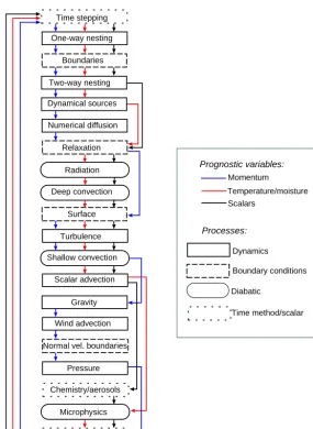
A schematic overview of one integration time step of the model, with the different processes affecting the prognostic variables, is presented in Fig. 2. The time stepping is applied with a parallel splitting approach, meaning that all process tendencies are computed from the same model state and then the sum of the tendencies is used to step forward.
3 Dynamical core and numerical schemes 3.1 Governing equations
The dynamical core of Meso-NH solves the conservation equations of momentum, mass, humidity, scalar variables,
and the thermodynamic equation derived from the conser-vation of entropy under the anelastic approximation. The temperature, density, and pressure are therefore described as small fluctuations from vertical reference profiles that are functions of height only. These equations are the same as in Lafore et al. (1998), in which further details can be found. The vertical coordinate is a height-based terrain-following coordinate. In addition to the originally implemented vertical coordinate (Gal-Chen and Somerville, 1975), it is also now possible to use the smooth-level vertical coordinate (SLEVE) (Schär et al., 2002) where small-scale features in the coor-dinate surfaces decay rapidly with height, limiting the exis-tence of steep coordinate surfaces to the lowermost few kilo-meters above the ground. For specific studies, it is possible to select a vertical domain that does not extend down to the ground, as in Paoli et al. (2014).
3.2 Transport schemes
Meso-NH is discretized on a staggered Arakawa C grid, where meteorological variables (temperature, water sub-stances, and TKE) and scalar variables are located in the center of the grid cell and the momentum components are located on the faces of the cells. Due to the C grid, the ad-vection schemes are different for these two types of variables. The transport schemes consider the equations in their flux form to ensure conservation:
∂
∂t(ρφ)e = − ∂
∂x(eρucφ)− ∂
∂y(eρvcφ)− ∂
∂z(eρwcφ), (1) where(x, y, z)are the transformed coordinates,eρis the dry density of the reference state,φis the variable to be trans-ported, including the wind components, and(uc, vc, wc)is the “advector ” field, corresponding to the contravariant com-ponents, i.e., the components of the wind orthogonal to the coordinate lines, due to the conformed horizontal projection and terrain-following vertical coordinates. In the Cartesian framework, the metric terms exactly cancel anduc,vc, and wcare equal tou,v, andw. For the sake of simplicity, only thex-derivative term is considered hereafter:
∂(eρucφ) ∂x =
∂(FC(eρuc)F (φ))
∂x . (2)
FC(eρUc)contains the topologic terms, which integrate the terrain transformations. The second fluxF (φ)is calculated on the mesh point without considering terrain transforma-tion, using the selected advection scheme.
The discrete form of the contravariant metric terms is sec-ond order in the horizontal directions and fourth order in the vertical direction in agreement with Klemp et al. (2003). The advection method for the wind variables and that for the scalars are distinct.
Time stepping
One-way nesting
Boundaries
Two-way nesting
Dynamical sources
Numerical diffusion
Relaxation
Radiation
Deep convection
Surface
Turbulence
Shallow convection
Chemistry/aerosols Scalar advection
Gravity
Wind advection
Normal vel. boundaries
Pressure
Microphysics
Online diagnostics
Momentum
Temperature/moisture Scalars
Dynamics
Diabatic
Boundary conditions
Time method/scalar
Prognostic variables:
Processes:
Figure 2.Flowchart of one integration time step of the simulation. The boxes represent the type of process, and the outline color represents the flows of the different types of variables.
is written such that ∂(eρucu)i
∂x =
FC(eρuc)i+1/2F (u)i+1/2 1x
−FC(eρuc)i−1/2F (u)i−1/2
1x . (3)
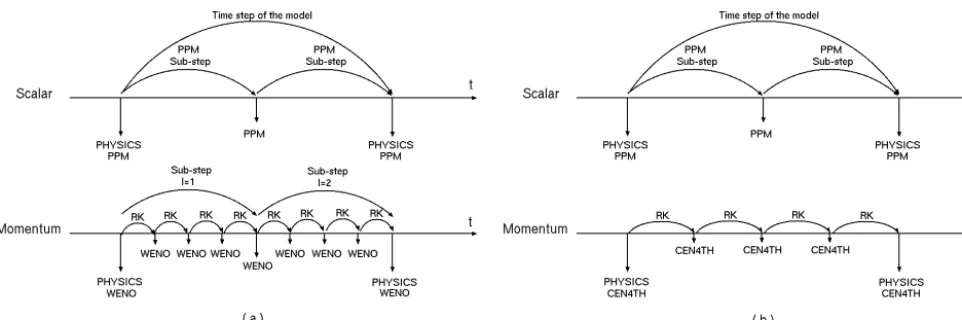
Two different methods with distinct orders can be used to discretizeF: a weighted essentially non-oscillatory (WENO) discretization of fifth or third order (WENO5 and WENO3, respectively), or a centered discretization of fourth order (CEN4TH), as detailed in Lunet et al. (2017). WENO schemes owe their success to the use of an adaptive set of stencils, allowing a better representation of the solution in the presence of high gradients (Shu, 1998; Castro et al., 2011). The major asset of the fourth-order centered scheme is its good accuracy (effective resolution on the order of 5–61x; Ricard et al., 2013).
The meteorological and scalar variable advection scheme is the piecewise parabolic method (PPM), in which piece-wise continuous parabolas are fitted in each grid cell, en-abling the scheme to handle sharp gradients and discontinu-ities very accurately. Three different versions of the PPM ad-vection scheme have been implemented in Meso-NH: the un-restricted PPM_00, the monotonic version, PPM_01, based on the original Colella and Woodward (1984) scheme with monotonicity constraints modified by Lin and Rood (1996), and PPM_02, a monotonic scheme with a flux limiter devel-oped by Skamarock (2006). All three versions have excellent mass-conservation properties.
3.3 Time integration
(ERK) methods can be applied to the momentum trans-port, and forward-in-time (FIT) integration is applied to the rest of the model, including PPM and the contravariant fluxFC(eρuc)transport. The different ERK methods are de-tailed in Lunet et al. (2017): the two main options are the fourth-order (RKC4) and the five-stage third-order (RK53) schemes.
To increase the maximum Courant–Friedrichs–Lewy (CFL) number, an additional time splitting can be activated for the wind advection with WENO. One time step[tn, tn+1] is divided into two regular sub-steps with a length of1t /2. The intermediate tendencies are computed using all stages of the ERK method, and the final tendency is the half sum of these two intermediate tendencies (Fig. 3a). The main in-terest of such an additional time splitting is to call the rest of the model (e.g., pressure solver, physics, and chemistry) less frequently: the larger time step is applied to the entire model including the physics and the pressure solver, with the FIT temporal scheme, while a smaller time step is used for the wind advection applying the ERK method on the subin-terval. Lunet et al. (2017) have shown that such an additional two-time splitting results in an improvement of the maximum CFL number while a three-time splitting results in no further improvements.
CEN4TH can be applied with the RKC4 time marching (Fig. 3b) or with the leapfrog (LF) scheme, using in the latter case, the Asselin filter to damp the computational temporal mode.
An additional time splitting can be activated for the scalar and meteorological variable advection to increase the time step of the rest of the model and to follow a CFL strictly less than 1 for the PPM (Fig. 3). This smaller time step for the PPM can evolve during the run as a function of the CFL number.
3.4 Numerical diffusion
The use of explicit numerical diffusion is prohibited with the PPM and WENO schemes. Only the fourth-order centered scheme for the momentum transport CEN4TH imposes a nu-merical diffusion operator for the wind to damp the numeri-cal energy accumulation in the shortest wavelengths, with the RKC4 or LF time integration. The diffusion operator applied to the wind components (u, v, w)is a fourth-order operator used everywhere except at the first interior grid point where a second-order operator is substituted in the case of nonpe-riodic boundary conditions. Details can be found in Lunet et al. (2017). The user fixes the time at which the 21xwaves are damped by the factore−1.
Meso-NH can also be used to reproduce experiments – in hydraulic tanks and flumes – characterized by a Reynolds number smaller than atmospheric ones by applying molec-ular diffusion to explicitly resolve the turbulence until the Kolmogorov scale is reached (Gheusi et al., 2000). Viscous diffusion terms are added to the momentum and heat
equa-tions: ∂
∂t(ρeU)= −ν∇(ρe∇U) (4) ∂
∂t(ρθ )e = −(ν/Pr)∇(eρ∇θ ), (5) whereUis the 3-D air velocity,Pr is the Prandtl number, de-fined as the ratio of the momentum diffusivity to the thermal diffusivity, andνis the kinematic viscosity.
3.5 Comparison of the momentum and temporal schemes
Because various spatial and temporal schemes are available for momentum transport, their choice depends on the in-tended use of the model and it is a compromise between the computing efficiency and the diffusive properties. A com-mon method to evaluate the diffusive behavior is to assess the effective resolution defined by the scale from which the slope of the model energy spectrum departs from the the-oretical one (Skamarock, 2004; Ricard et al., 2013). Fig-ure 4 displays the kinetic energy spectra for the FIRE stra-tocumulus case at a resolution of 1x=50 m for the spa-tial and temporal schemes available in Meso-NH. It shows that CEN4TH/RKC4 presents a remarkably effective res-olution (on the order of 41x), followed by CEN4TH/LF (∼61x), and then WENO5/RK53–RKC4 (∼81x), with the most diffusive being WENO3 (∼101x). Mazoyer et al. (2017) found similar results for the fog case. Some recom-mendations for numerical schemes are summarized in Ta-ble 1. CEN4TH/RKC4 is recommended for LES of clouds because the entrainment of environmental air at the cloud edges is higher with CEN4TH/RKC4 due to lower implicit diffusion, whereas WENO3 is inappropriate because it is ex-cessively damping. However, WENO3 presents the best wall-clock time to solution and is recommended for long climate simulations for which the turbulence and cloud processes are fully parameterized. WENO5/RK53–RKC4 is well adapted to sharp gradient areas (Lunet et al., 2017), e.g., in com-plex shock–obstacle interactions with the immersed bound-ary method and in mesoscale case studies. The RK53 and RKC4 temporal schemes associated with WENO5 produce similar results.
3.6 Initial and boundary conditions
Figure 3.Representation of the time marching in Meso-NH with(a)WENO5/RKC4 and(b)CEN4TH/RKC4 for the momentum transport.
Table 1.Recommendations for the choice of wind transport and temporal schemes according to the applications.
Wind transport scheme Temporal scheme Applications
CEN4TH RKC4 LES
WENO3 RK53 or RKC4 Climate – chemistry
WENO5 RK53 or RKC4 Mesoscale – sharp gradients
Figure 4. FIRE stratocumulus simulation case (1x=50 m) at 11:00 LT (local time) on 14 July 1987: mean kinetic energy spec-tra for the vertical wind computed in the boundary layer (between 0 and 1100 m) with different numerical schemes for the wind trans-port. The dashed line indicates the power law with an exponent of −5/3 (the Kolmogorov spectrum).
(Global Forecast System). Initialization from ECMWF re-analyses is also possible. For ideal case studies, an initial vertical profile usually derived from observed radiosounding data can be provided by the user to be interpolated horizon-tally and vertically onto the Meso-NH grid to serve as ini-tial and LS fields. The different forcing methods classically used in model intercomparison exercises, from geostrophic
winds to large-scale thermodynamical tendencies, are imple-mented in the code. Mostly used for long-duration simula-tions, a nudging of the wind components, potential temper-ature, and vapor mixing ratio towards the LS fields can be applied. In addition, an attribution method of filtering and bo-gussing has been introduced to the Meso-NH code to replace an ill-defined vortex in a LS field (Nuissier et al., 2005) or to isolate individual features from an ambient flow for further investigation (Pantillon et al., 2013). This method (Nuissier et al., 2005) consists of first filtering the LS fields of the wind, temperature, and humidity following the approach of Kuri-hara et al. (1993) and then adding the studied features or vor-tex to the likely filtered environmental conditions deduced from observations.
The lateral boundary conditions can be cyclic, rigid wall, or open and are detailed in Lafore et al. (1998). One change from the reference paper concerns the Carpenter method ap-plied to the normal velocity componentun:
∂un ∂t =
∂u n ∂t
LS
−C∗ ∂u
n ∂x −
∂u n ∂x
LS
Figure 5. Physical parameterizations available in Meso-NH. The left-hand parameterizations are based on the implicit assumption because the processes they represent occupy only a portion of each grid mesh. The right-hand parameterizations represent several subgrid-scale processes that can be active over the full portion of each grid mesh.
for the interior value (0.8), while they were taken to be the LS values in the reference paper.
The ceiling of the model is rigid, corresponding to a free-slip condition. An absorbing layer can be added to prevent the reflection of gravity waves on this lid, where the prognos-tic variables are relaxed towards the LS fields. The bottom boundary considers a free-slip condition (u.n=0). When performing direct numerical solution with Meso-NH, it is also possible to consider a no-slip bottom boundary condi-tion (u(z=0)=0).
4 Physical parameterizations
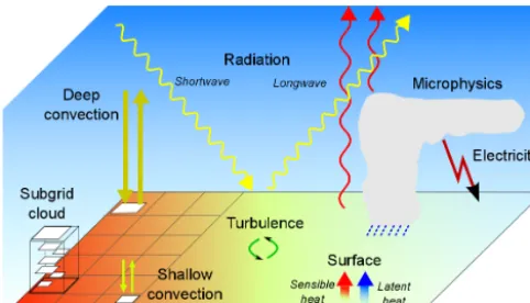
In this section, a description of the physical parameteriza-tions present in Meso-NH (Fig. 5) is given. We focus on the most recent developments and some specific applications that are currently of great interest. Figure 6 summarizes the avail-able schemes, and the links between them.
4.1 Surface
The surface schemes, initially available in Meso-NH, have been externalized to create SURFEX (Surface externalisée) standardized surface platform (Masson et al., 2013a); these schemes have since been enhanced by the contributions of different coupled models (from LES scale with Meso-NH to global climate simulation). Each grid box is split into four tiles: land, town, sea, and inland water (lakes and rivers). The main in-line schemes are the interactions between soil, bio-sphere, and atmosphere (ISBA) parameterization (Noilhan and Planton, 1989), the town energy budget (TEB) scheme used for urban areas (Masson, 2000), and the freshwater lake model (FLake) used for lake surfaces (Mironov et al., 2010). Recently, a standard coupling interface was introduced to SURFEX (Voldoire et al., 2017) enabling coupling with
var-ious ocean and wave models to compute air–sea fluxes over the sea water tiles. The principle for the four tile types is that, during a Meso-NH time step, each surface grid box re-ceives the potential temperature, vapor mixing ratio, horizon-tal wind components, pressure, tohorizon-tal liquid and solid precip-itation, longwave (LW), shortwave (SW), and diffuse radi-ation, and possibly concentrations of chemical and aerosol species from the first atmospheric level above the ground. SURFEX returns the averaged fluxes for the sensible and la-tent heat, momentum, chemistry, and aerosols, as well as the radiative surface temperature, and surface direct and diffuse albedo and surface emissivity, which are used at the same first atmospheric level above the ground by the turbulence and radiation schemes. The coupling method can be applied to any data flow between the soil and the atmosphere. Note that it is also possible to prescribe the energy fluxes and roughness length, possibly separately for each tile, to be able to perform theoretical studies, such as LES intercomparisons. The vegetation scheme ISBA represents the effect of both vegetation and bare soil. The high vegetation can be simu-lated either as a separate layer above low vegetation, or as the more traditional and simplistic way of the “slab” (all the veg-etation being then placed at ground level). Several evapotran-spiration formulations are available for plants, the most ad-vanced taking into account photosynthesis, respiration, and plant growth, and being able to simulate CO2fluxes as well. The soil is described either as a bucket of two or three lay-ers or with a discretization in many (typically 14) laylay-ers, in which a root profile is defined. Freezing of the soil water is simulated, as well as snow mantel, with various degrees of complexity (the most complex snow scheme having many snow layers and simulating the evolution of the macro- and microphysical characteristics of the snow). Permanent snow is treated in the ISBA scheme as very deep snow. The land tile can be separated into up to 19 subtiles, defined by the plant functional types, in order to perform more accurate veg-etation and soil simulations, especially when photosynthesis and plant growth is simulated.
SURFEX Chemistry
Radiation
Turbulence Aerosols
chemistry
Microphysics
Subgrid cloud scheme
Deep convection
Shallow & dry convection
ISBA TEB
SEA
CROCUS 1-D ocean
Flake Electricity
Dust & sea salt Near-surface snow transport
Forefire 3-D ocean
Figure 6.Physical and chemical schemes and the one-way or two-way links among them. Black arrows represent the direct interaction among schemes, orange arrows the indirect interaction through fluxes or cloud fraction, and green arrows the subgrid transport of prognostic variables.
and building architecture influence these heat emissions in the model.
The FLake scheme models the structure of the mixed and stratified water layers within the lakes using an assumed parametric form of the temperature profile. The effect of the sediment layer below the water is also considered, as well as the ice (and snow) above the water.
For the exchanges over sea surfaces, the surface fluxes are parameterized for a wide range of wind and environmental conditions, from low winds to hurricanes (Belamari and Pi-rani, 2007). There is the possibility of using a coupled 1-D ocean model. The single column model takes into account the vertical mixing within the ocean, as well as radiation absorp-tion and surface energy balance. Also, the coupling with a 3-D model, more detailed in Sect. 7.1, is carried out through SURFEX. It allows the addition of the advection processes and the sea currents, at different scales. A wave model can also be activated, further modifying the surface fluxes. Sea ice is treated either where sea surface temperature is below −4◦C or by the GELATO sea ice model (Mélia, 2002) cou-pled with a 3-D ocean model.
Meso-NH version 5.4 includes SURFEX version v8.1. For a standard use of Meso-NH with SURFEX, four data files are needed for the orography, clay and sand soil textures, and land use from ECOCLIMAP (Faroux et al., 2013) and ECOCLIMAP second generation. Global databases at 300 m (land cover, plant functional types, urban local climate zones
(Stewart and Oke, 2012), vegetation parameters as leaf area index) and 1 km resolution (soil composition, lake depths, etc.) are available on the Meso-NH web site. All parameters can also be prescribed separately by the user, as can the sur-face fluxes in an idealized configuration.
4.2 Turbulence
The turbulence scheme is based on Redelsperger and Som-meria (1982, 1986) and implemented in Meso-NH according to Cuxart et al. (2000a).
The scheme is built on the diagnostic expressions of the second-order turbulent fluxes, using the two quasi-conservative variables first introduced by Betts (1973) and Deardorff (1976), the liquid-water potential temperatureθl, and the non-precipitating total water mixing ratiort=rv+ rc+ri:
u0iθl0= −2 3
L Cs
e12 ∂θl
∂xi
φi, (7)
u0irt0= −2 3
L Ch
e12 ∂rt
∂xi
ψi, (8)
u0iu0j=2 3δije−
4 15
L Cm
e12
∂ui ∂xj
+∂uj ∂xi
−2 3δij
∂um ∂xm
and primes correspond to means and turbulent components, respectively.
The turbulence scheme includes the prognostic equation of the subgrid turbulent kinetic energye, closed by the mixing length L, the dissipation being proportional to the subgrid TKE:
∂e ∂t = −
1 e ρ
∂ ∂xj e
ρeuj−u0iu0j ∂ui ∂xj
+ g e θv
u03θ0 v +1 e ρ ∂ ∂xj
C2meρLe
1 2 ∂e
∂xj
−C e32
L. (10)
ui is theith component of the velocity,θvthe virtual poten-tial temperature,eθv the virtual potential temperature of the reference state,gthe gravitational acceleration, andC2mand Cconstants.
At mesoscale resolutions (horizontal mesh larger than 2 km), it can be assumed that the horizontal gradients and the horizontal turbulent fluxes are much smaller than their verti-cal counterparts: therefore, they are neglected (except for the advection of TKE) and the turbulence scheme is used in its 1-D version (noted T1-D), as in AROME (Seity et al., 2011). At finer resolution, the entire subgrid equation system in its 3-D version is considered (noted T3-D), allowing LESs on flat or heterogeneous terrains.
In the same way, the mixing length is diagnosed differ-ently in the mesoscale and LES modes. At coarse resolution (typically greater than 500 m), the mixing length is related to the distance an air parcel can travel upwards (lup) and down-wards (ldown), constrained between the ground and the ther-mal stratification (Bougeault and Lacarrère, 1989). However, this mixing length, first built and evaluated for convective boundary layers, is unrealistic in purely neutral conditions (the upward length goes to the model top). In neutral but also stable conditions, the vertical wind shear constitutes the only positive source of TKE and is of primary importance to influence turbulent eddies. Rodier et al. (2017) proposed a buoyancy-shear combined mixing length by adding a local vertical wind shear term to the nonlocal effect of the static stability.
The mixing length for Bougeault and Lacarrère (1989) and Rodier et al. (2017) is defined by
L= "
(lup)−2/3+(ldown)−2/3 2
#−3/2
. (11)
The distanceslupandldownare defined by
z+lup
Z z
g eθv
(θ (z0)−θ (z))+C0 √
eS(z0)
dz0= e(z), z
Z z−ldown
g eθv
(θ (z)−θ (z0))+C0 √
eS(z0)
dz0= e(z), (12)
with S= s ∂u i ∂z 2 + ∂u j ∂z 2 . (13)
Note that Bougeault and Lacarrère (1989) formulas corre-spond toC0=0.
When used in T3-D mode, the horizontal mixing lengths are equal to the vertical one. In LESs, the mixing length can be linked to the largest subgrid eddies, which have the size of a nearly isotropic grid cell:
L=(1x1y1z)1/3. (14)
With strong stratification, these eddies are smaller; therefore, a mixing length reduced by stratification according to Dear-dorff (1980) is proposed:
L=min
(1x1y1z)1/3,0.76 q
e/N2
, (15)
whereNis the Brunt–Väisälä frequency.
Near the ground, the length scales of the subgrid tur-bulence scheme are modified according to Redelsperger et al. (2001) to match the similarity laws and the free-stream model constants. T1-D or T3-D and the mixing length parametrization are chosen by the user according to clear rec-ommendations given above.
To better represent the flow dynamics near the ground in the presence of complex plant or urban canopies, LESs are now frequently performed with meter-scale vertical resolu-tion. Classically, the influence of these elements on the dy-namics is introduced by the surface scheme via a roughness approach. A more realistic method is the drag approach (Au-mond et al., 2013) in which drag terms are added to the mo-mentum and subgrid TKE equations as a function of the fo-liage density for plant canopies:
∂α ∂tDRAG
= −CdAf(z)α p
u2+v2, (16)
withα=u, v,or e, whereuandv are the horizontal wind components, Cd is the drag coefficient, and Af(z) is the canopy area density.
Inside convective clouds, Verrelle et al. (2015) have shown that turbulent mixing is insufficient in the updraft core, espe-cially at coarse resolution (2 km), leading to strong resolved vertical velocities, even though it is better in T3-D than in T1-D (Machado and Chaboureau, 2015). LESs of convective clouds have shown that thermodynamical counter-gradient structures are present in convective clouds, as they are in con-vective boundary layers, and cannot be intrinsically repre-sented by the common eddy-diffusivity turbulence scheme at mesoscale (Verrelle et al., 2017). The same study succeeded in reproducing the counter-gradient structures and increas-ing the thermal production of the TKE with the approach proposed by Moeng (2014), which parameterizes the verti-cal thermodynamiverti-cal fluxes in terms of horizontal gradients of resolved variables. Conversely, the necessity of increas-ing turbulence at the cloud edges remains an active field of research.
4.3 Convection and dry thermals
At horizontal resolutions coarser than 5 km, it is necessary to parameterize both shallow and deep convective clouds. One deep convection scheme and two shallow convection schemes are available in Meso-NH. The deep convection scheme, called KFB, is based on Kain and Fritsch (1990) with some adaptations presented in Bechtold et al. (2000). KFB can also be applied to shallow cumuli, but it is not efficient enough, and does not represent dry thermals. An-other mass flux formulation of convective mixing, proposed in the eddy-diffusivity mass flux approach (Hourdin et al., 2002; Soares et al., 2004), addresses this issue and has been introduced by Pergaud et al. (2009) into Meso-NH, called PMMC09. This formulation considers a single entraining– detraining rising parcel starting from the ground. The vertical velocity equation is given by
wu ∂wu
∂z =aBu−bw 2
u, (17)
wherewuis the vertical velocity inside the updraft,Buis the buoyancy, is the entrainment rate, anda and b are con-stants. Entrainment and detrainment rates in the dry updraft are given by
dry=max
0, C Bu w2 u
, (18)
and δdry=max
1
lup−z , Cδ
Bu w2 u
, (19)
whereC andCδ are constants. Mass flux continuity is en-sured at cloud base between the dry and moist parts of the updraft. In the moist part, entrainment and detrainment rates are derived from the buoyancy sorting approach of Kain and Fritsch (1990). The closure assumption is given by the up-draft initialization at the surface.
PMMC09 is also used in AROME at resolutions of 2.5 km and now 1.3 km and has considerably improved the real-ism of the clouds and winds in the PBL as shown by Lac et al. (2008) and Seity et al. (2011). A comparison among PMMC09 and five other mass-flux schemes using the AROME framework on the five French metropolitan ra-dio sounding locations over 1 year in Riette and Lac (2016) demonstrated the good performance of this scheme, which was characterized by the active transport of thermals. In con-vective situations, a deep convection scheme is not necessary anymore below 5 km resolution, but it is still necessary to use a mass-flux scheme such as PMMC09 until 1 km–500 m horizontal grid spacing. However, in this range of grid spac-ing, PBL thermals may be partly resolved and partly sub-grid because they are in the grey zone of turbulence (Honnert et al., 2011). Honnert et al. (2016) showed that the mass-flux scheme, in its original form, is too active at this range of res-olution, preventing the production of resolved structures, and proposed several modifications to adapt PMMC09 to the grey zone.
4.4 Microphysics
Different bulk microphysical schemes are available in Meso-NH that predict either one or two moments of the particle size distribution for a limited number of liquid or solid wa-ter species. One-moment microphysical schemes predict the mass mixing ratio of some water species, and two-moment schemes predict both the mass mixing ratio and the number concentration of some species.
The most commonly used one-moment scheme is the mixed ICE3 scheme (Caniaux et al., 1994; Pinty and Jabouille, 1998) including five water species (cloud droplets, raindrops, pristine ice crystals, snow or aggregates, and grau-pel), coupled to a Kessler scheme for warm processes. Hail is considered either as a full sixth category (providing the ICE4 scheme; Lascaux et al., 2006) or as forming with graupel an extended class of heavily rimed ice species. ICE3 is included in this latter form in AROME (Seity et al., 2011). The particle sizes for each category follow a generalized Gamma distri-bution, with the particular case of the exponential Marshall– Palmer distribution for the precipitating species. Power-law relationships allow the mass and fall speed to be linked to the particle diameters. Cloud species are also handled by the subgrid transport (turbulence and shallow convection with PMMC09). Numerous processes exchanging mass among species are presented in Lascaux et al. (2006). All the mi-crophysical processes are computed independently of each other with a mass budget at each step to ensure conserva-tion. Following the microphysics, an implicit adjustment of the temperature, vapor, cloud, and ice contents is performed in clouds with a strict saturation criterion.
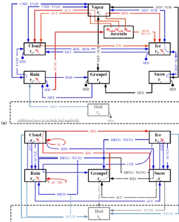
with the two-moment warm microphysical scheme from Co-hard and Pinty (2000a, b). In addition to the five water mixing ratios of ICE3, LIMA predicts the number concentration of the cloud droplets, raindrops, and pristine ice crystals. The strength of the scheme is that it includes a prognostic rep-resentation of the aerosol population, which is represented by the superimposition of several aerosol modes, each mode being defined by its chemical composition, particle size dis-tribution, and ability to act either as cloud condensation nu-clei (CCN), ice-freezing nunu-clei (IFN), or coated IFN (aged IFN acting first as CCN and then as IFN) as a function of its solubility. As in ICE3, LIMA assumes a thermodynami-cal equilibrium between the water vapor and cloud droplets. However, in the cold phase, the prediction of the concentra-tion of ice crystals leads to an explicit computaconcentra-tion of the deposition and sublimation rates, allowing under- or super-saturation over ice. The microphysical processes of ICE3– ICE4 and LIMA are summarized in Fig. 7. The names of the processes are given in Table 2.
A variant to this scheme has been introduced by Geof-froy et al. (2008) for low precipitating warm clouds pro-ducing drizzle, following Khairoutdinov and Kogan (2000). Instead of a diagnostic saturation adjustment for the warm phase, Thouron et al. (2012) proposed, for LESs of boundary layer (BL) clouds, a pseudo-prognostic approach for super-saturation to limit the droplet concentration production and to better represent cloud-top supersaturation due to mixing between cloudy and clear air.
The two-moment microphysical approach in Meso-NH has allowed numerous studies of the impact of aerosols on cloud life cycles to be conducted, e.g., for cumulus clouds (Pinty et al., 2001), stratocumulus clouds (Sandu et al., 2008, 2009), and fog (Stolaki et al., 2015).
4.5 Subgrid cloud schemes
When the spatial resolution is not sufficient to consider the grid mesh to be completely clear or cloudy, a subgrid con-densation scheme can be activated with one-moment micro-physical schemes, as suggested by Sommeria and Deardorff (1977) and Mellor (1977), supplying a cloud fraction to the radiation scheme. The statistical cloud scheme is based on the computation of the variance of the departure to the satu-ration inside the grid box, summarizing both the temperature and total water fluctuations. PDFs of the saturation deficit are used to represent the statistical distribution of the cloud vari-ability, and the cloud fraction and mean cloud water mixing ratio can be deduced. A combination of unimodal Gaussian and skewed exponential PDFs is defined for BL clouds ac-cording to Bougeault (1981, 1982). Chaboureau and Bech-told (2002, 2005) introduced the effects of a deep convec-tion scheme in the parameterizaconvec-tion of the standard devia-tion of the saturadevia-tion deficit. The subgrid variability from the PMMC09 shallow convection scheme can be introduced in the same way via the variance of the saturation deficit,
Table 2.List of the microphysical processes.
Symbol Process
ACC Accretion (e.g., of droplets by rain drops)
ACT CCN activation
AGG Aggregation of pristine ice on snow
AUTOC Autoconversion of cloud droplets into rain drops AUTOI Autoconversion of pristine ice crystals into snow
BER Bergeron–Findeisen
CFR Rain contact freezing CND/EVAP Condensation and evaporation DEP/SUB Deposition and sublimation
DRYG/WETG Growth of graupel in the dry or wet regimes HEN Heterogeneous nucleation on IFN
HM Hallett–Mossop
HON Homogeneous freezing
IFR Immersion freezing of coated IFN
MLT Melting
RIM Cloud droplet riming on snow SC Self collection of cloud droplets SC/BU Self collection and breakup of rain drops SCAV Below-cloud aerosol scavenging by rain
SED Sedimentation
SHED Water shedding
WETH Growth of hail in the wet regime
or the cloud fraction can be diagnosed directly from the updraft fraction. The second method has been chosen for the operational version of AROME. Perraud et al. (2011) have conducted a statistical analysis with Meso-NH of LESs of warm BL clouds to show that double Gaussian distribu-tions are more appropriate than unimodal theoretical PDFs when describing sparse subgrid clouds such as shallow cu-muli and fractional stratocucu-muli, in agreement with Larson et al. (2001a, b) and Golaz et al. (2002a, b). Because there can be other sources of subgrid variability, such as gravity waves in stable BL clouds, when the turbulence and shallow convective contributions are too weak to produce clouds, a variance proportional to the saturation total water specific hu-midity has been added, as in classical relative huhu-midity cloud schemes (e.g., Rooy et al., 2010), and has shown significant improvement for winter clouds in AROME.
In the same way, a subgrid rain scheme has been devel-oped by Turner et al. (2012) to simulate the gradual transi-tion from non-precipitating to fully precipitating model grids for warm clouds. A prescribed PDF of cloud water variabil-ity and a threshold value of the cloud mixing ratio for droplet collection are used to derive a rain fraction, and overlapping assumptions for the cloud and rain fraction are considered. In the future, this approach will be generalized to mixed micro-physical processes, and the PDFs between the subgrid cloud and rain schemes will be harmonized.
4.6 Radiation
Figure 7.Diagrams of the microphysical processes of ICE3–ICE4 and LIMA:(a)all the processes except collection;(b)collection processes. Blue arrows represent existing processes in ICE3 modified in LIMA, red arrows are new processes in LIMA, and black arrows are identical processes in ICE3 and LIMA. When hail is a full sixth category (in ICE4 and LIMA), processes are in muted colors. Prognostic variables for all the hydrometeor species are written in the boxes, withrthe mixing ratio andNthe concentration.
radiation code calculates the atmospheric heating rates and the net surface radiative forcing required to compute the tem-poral evolution of the potential temperature and the surface energy balance:
∂θ ∂t =
g Cph
5∂F
∂p, (20)
whereF is the net total flux:F =F↑LW+FLW↓ +F↑SW+F↓SW sum of the upward and downward SW and LW fluxes, and Cphthe calorific capacity. In addition it returns the SW and
LW fluxes at each model level as diagnostics in a number of spectral bands, distinguishing between the direct and diffuse components for SW. Clear-sky quantities are also available. LW and SW radiative transfers are treated by distinct rou-tines.
inte-grating 16 bands and 140 g points (Morcrette, 2002). The SW radiation scheme applies the photon path distribution method employed by Fouquart and Bonnel (1980) in six spectral bands. The total cloud fraction is computed according to the cloud overlap assumption, and fluxes are calculated indepen-dently in the clear and cloudy portions before being aggre-gated.
The latest radiation code of ECMWF, ecRad (Hogan and Bozzo, 2016), was implemented in Meso-NH in 2017. This code is highly modular, which allows the user to conveniently choose between multiple options. The main differences from the original code concern the implementation of the SW ver-sion of RRTM with 14 bands and 112 g points (Morcrette et al., 2008) and some modifications regarding the treatment of unresolved cloud horizontal heterogeneities. The latter can now be treated with the McICA (Pincus et al., 2003) or TripleClouds (Shonk and Hogan, 2008) methods, or with the SPARTACUS solver (Schäfer et al., 2016; Hogan et al., 2016), which represents lateral photon transport through the cloud sides (Hogan and Shonk, 2013) in a 1-D formalism. The overall code has also been rewritten, resulting in a 30 % reduction in the computation time compared to the origi-nal configuration. Aerosols are now prescribed via the mix-ing ratio vertical profiles of 12 different aerosol types cor-responding to various physical properties and sizes accord-ing to CAMS (the Copernicus Atmosphere Monitoraccord-ing Ser-vice; Stein et al., 2012). The optical properties of hydrophilic aerosols change with relative humidity, and their mixing ra-tios can be prognostic, or taken from the CAMS climatology (Bozzo et al., 2017), which replaces the former six-class cli-matology of Tegen et al. (1997) that used optical properties from Aouizerats et al. (2010).
In both radiative codes, liquid and ice cloud optical proper-ties can be computed according to a variety of parameteriza-tions. The liquid cloud optical radius is generally computed from the liquid water content following the parameterization of Martin et al. (1994) for the one-moment microphysical scheme, while it is deduced from the particle size distribution in two-moment microphysics. Likewise, the ice cloud optical radius can be computed from the ice water content following Sun and Rikus (1999) and Sun (2001). Cloud optical proper-ties (optical depth, single-scattering albedo, and asymmetry parameter) are then computed as a function of the particle effective radius following the parameterizations of Fouquart (1988) or Slingo (1989) for one-moment schemes, and Sav-ijärvi et al. (1997) for two-moment schemes. Ice water opti-cal properties can be computed according to Ebert and Curry (1993), Smith and Shi (1992), and Baran et al. (2014). 4.7 Electricity
Meso-NH is one of three CRMs with a completely explicit 3-D electrical scheme. The scheme, called CELLS for the cloud electrification and lightning scheme (Barthe et al., 2012), computes the full life cycle of the electric charges
from their generation to their neutralization via lightning flashes. An earlier version of this scheme (Molinié et al., 2002; Barthe et al., 2005) was gradually improved in order to cope with simulations of thousands of lightning flashes over large grids and complex terrain (Barthe et al., 2012). It was developed from the one-moment bulk mixed-phase mi-crophysics scheme ICE3 and its extension hail ICE4. The scheme follows the evolution of the mass charge density (qx in C kg−1of dry air) attached to each condensate species of the microphysics scheme:
∂
∂t(ρqex)+ ∇ ·(ρqexU)=eρ(S q
x+Txq). (21) The source terms Sqx include the turbulence diffusion, the charging mechanism rates, the charge sedimentation by grav-ity, and the charge neutralization by lightning flashes.Txq is the transfer rates due to the microphysical evolution of the particles.
CELLS follows the positive and negative ion concentra-tions (n± in kg−1), whose governing equation includes the
drift in the electric field, the attachment to the charged hy-drometeors, the release of ions when hydrometeors evapo-rate or sublimate, production via lightning flashes and via point discharge current from the surface, ion generation via cosmic rays, and ion–ion recombination. Fair weather condi-tions are computed following Helsdon and Farley (1987) and are used to initialize the positive and negative ion concentra-tion profiles and to treat the lateral boundary condiconcentra-tions.
The cloud electrification is based upon the common as-sumption that the charge separation in thunderstorms mainly occurs during rebounding collisions between more or less rimed particles. However, there is still no consensus on the theory of so-called noninductive charging mechanisms. Therefore, several parameterizations of this process have been implemented into CELLS as described in Barthe et al. (2005). This set of parameterizations includes the well-known equations of Takahashi (1978), Saunders et al. (1991), and Saunders and Peck (1998), along with some improve-ments by Tsenova et al. (2013). The inductive process, which is efficient once an electric field is well established in the clouds, can also be activated (Barthe and Pinty, 2007a). Elec-tric charges are exchanged between hydrometeors during mass transfers due to microphysical processes. Each electric charge transfer rate is associated with a mass transfer rate in proportion to the electric charge density and inverse mixing ratio.
The electric field (E) is computed from the Gauss equation forced by the total charge volume density (ρtot):
∇ ·E=ρtot
, (22)
Meso-NH:
E= −∇V . (23)
Eis then derived using a numerical gradient operator. The lightning flash scheme was designed to reproduce the overall morphological characteristics of the flashes at the model scale. Indeed, an accurate estimate of the lightning path would computationally be too expensive when simu-lating real meteorological cases over large domains (Barthe et al., 2012). In order to treat several flashes in the same time step, an iterative algorithm was developed to identify and de-lineate all the electrified cells in the domain. A lightning flash is triggered once the electric field in an electrified cell reaches a threshold value (Etrig) that decreases with altitude as given by Marshall et al. (2005). In the first step, the flash propagates vertically as the bidirectional leader. In the second step, and to account for the horizontal extension highlighted by very-high-frequency (VHF) mapping systems, a branching algo-rithm allows the 3-D structure of the lightning flashes to be mimicked. As a result the grid point locations reached by the lightning “branches” are estimated according to a fractal law (Niemeyer et al., 1984).
The total charge in excess of|0.1|nC kg−1is neutralized along the lightning channel. In the case of intra-cloud flashes, a charge correction is applied to all the flash grid points to ensure an exact electroneutrality prior to the redistribution of the net charge to the charge carriers at the grid points. This constraint does not apply to cloud-to-ground discharges (charge leakage in the ground), which are defined when the tip of the downward branch of the leader reaches an altitude below 2 km above ground level. Once charge neutralization is completed, the electric field is updated. If a new triggering point is found in at least one of the detected cells, a new light-ning flash is triggered. This allows several lightlight-ning flashes to occur during a single time step.
A lightning-produced NOx (LNOx) parameterization is implemented in the electrical scheme. Since the CELLS scheme reproduces the lightning flash path, the LNOx pro-duction is taken proportional to the lightning flash length and depends on the atmospheric pressure (Barthe et al., 2007b).
5 Chemistry and aerosols
Meso-NH integrates a complete set of processes to simu-late changes in the atmospheric composition in terms of aerosols and trace gases from LES to continental scales. Ini-tial and boundary conditions for gases and aerosols are pro-cessed following the same procedure as the dynamical vari-ables (Sect. 3.6). For real-case studies, LS chemical fields are provided by two global models: Modèle de Chimie At-mosphérique à Grande Echelle (MOCAGE; Bousserez et al., 2007) and the Model for OZone And Related chemical Trac-ers (MOZART; Emmons et al., 2010). For ideal case studies,
a user-prescribed horizontally homogeneous vertical profile is applied.
5.1 Emissions and dry deposition
The interactions of gases and aerosols with the surface are treated in the externalized surface model SURFEX (Sect. 4.1). Dry deposition processes commonly follow the resistance analogy described by Wesely (1989) and take into account the aerodynamic and canopy resistances as a func-tion of land cover types and vegetafunc-tion. A full descripfunc-tion is given by Tulet et al. (2003). Dry deposition and sedimenta-tion of aerosols are driven by Brownian diffusivity and the gravitational velocity. These processes are calculated over each mode of the aerosol size distribution (Tulet et al., 2005). For the sedimentation process, the gravitational velocity is solved using a time-splitting technique to compute the sedi-mentation fluxes. Emissions for the model domain are com-plied from a prescribed emissions database or can be pa-rameterized. The surface model can process the raw pre-scribed emission data from any inventory of primary gases or aerosols. Emissions can include urban and industrial, bio-genic, biomass burning, and volcanic sources from the most recent emissions databases. Desert dust emissions are pa-rameterized following the Dust Entrainment and Deposition model (DEAD; Zender et al., 2003) based on the pioneering work of Marticorena and Bergametti (1995). The dust emis-sion scheme was incorporated into Meso-NH–SURFEX by Grini et al. (2006) and modified by Mokhtari et al. (2012) to better account for the size distribution of erodible mate-rial. Sea salt emission follows the parameterization of Ovad-nevaite et al. (2014). Input parameters such as wind stress, significant wave height, salinity, and sea surface temperature are taken from oceanic models such as CROCO (Coastal and Regional Ocean COmmunity model; Debreu et al., 2016) or NEMO (Nucleus for European Modelling of the Ocean; Madec, 2008) and from the wave model WW3 (WAVE-WATCH III; Tolman, 2009). A more detailed presentation of coupling over water is provided in Sect. 7.1. Biogenic emissions are either prescribed or calculated online based on the Model of Emissions of Gases and Aerosols from Na-ture (MEGAN) version 2.1 (Guenther et al., 2012), which has been integrated into Meso-NH.
5.2 Chemistry
simu-lations whereas the Rosenbrock solvers are more adapted to address the increase in the system stiffness for cloud chem-istry simulations. Photolysis rate coefficients are computed using the TUV (tropospheric ultraviolet and visible radia-tion) model version 5.3.1 (Madronich and Flocke, 1999), which can be used online or offline. In order to limit the computational time in 3-D simulations, photolysis rates are computed at the first time step for a discrete number of solar zenith angles and altitudes, using ozone and aerosol clima-tologies, and for clear-sky conditions. The choice of ozone and aerosol climatologies is flexible. Cloud correction of tabulated clear-sky values follows Chang et al. (1987) and Madronich and Flocke (1999). In 0-D or 1-D, the TUV model is used online and takes explicitly into account the prognostic ozone and aerosol distributions.
5.2.1 Gas-phase chemistry
Several chemical mechanisms are available in Meso-NH (Table 3). The RACM (Regional Atmospheric Chemistry Mechanism; Stockwell et al., 1997) and CACM (Caltech Atmospheric Mechanism; Griffin et al., 2002) mechanisms are largely used in 3-D atmospheric chemistry 3-D mod-els. The latter is particularly appropriate for the production of semi-volatile precursors of secondary organic aerosols (SOAs). Two reduced versions were developed for Meso-NH based on these baseline reaction mechanisms: ReLACS (Regional Lumped Atmospheric Chemical Scheme; Crassier et al., 2000) and ReLACS2 (Regional Lumped Atmospheric Chemical Scheme version 2; Tulet et al., 2006), respectively. 5.2.2 Aerosol module
The different components of the aerosol module ORILAM (Organic Inorganic Lognormal Aerosols Model) are de-scribed in Tulet et al. (2005). Only a brief summary of the most important features is given here. A lognormal size dis-tribution function is applied to represent the Aitken, accu-mulation, and coarse modes. The prognostic evolution of the aerosol size distribution considers three moments for each mode (the zeroth, third, and sixth) to compute the evolution of the total number, number median diameter, and geomet-ric standard deviation. Desert dust and sea salt aerosols are described by three and five lognormal modes, respectively, with a prescribed chemical composition. The size distribu-tion and the chemical composidistribu-tion of anthropogenic aerosols are defined using two lognormal functions for the Aitken and accumulation modes. For these aerosols the chemical mixing is internal and, for each mode, the model computes the evo-lution of the primary species (black carbon and primary or-ganic carbon), three inoror-ganic ions (NO−3,SO24−,NH+4), the condensed water, and the 10 SOA classes.
The most important process for the formation of SOA is the homogeneous nucleation in the sulfuric acid–water sys-tem. It is based on the Kulmala et al. (1998)
parameteriza-tion, consistent with the classical theory of binary homoge-neous nucleation (Wilemski, 1984), and integrates the hy-dration effect. The newly formed particles are added to the Aitken mode of anthropogenic particles. The aerosol size distribution evolves via collision between particles, leading to a coagulation process. Both intramodal and intermodal coagulations are taken into account. Changes in the lognor-mal distribution are calculated based on Whitby et al. (1991) but modified to allow a particle resulting from two particles colliding within the Aitken mode to be assigned to the ac-cumulation mode. Anthropogenic aerosols are fully coupled with the gas-phase chemistry, allowing subsequent interac-tions with gaseous source precursors. The ORILAM scheme assumes that the aerosols are old enough to have a short liq-uid film at the surface, which favors the absorption process. An inorganic chemistry system calculates the chemical com-position of sulfate–nitrate–water–ammonium aerosols based on equilibrium thermodynamics. Several solvers are im-plemented such as ARES (Binkowski and Shankar, 1995), ISORROPIA (Nenes et al., 1998), and EQSAM (Metzger et al., 2002). For organics, ORILAM uses the MPMPO scheme (Griffin et al., 2003; Dawson and Griffin, 2016) cou-pled with the CACM or ReLACS2 chemical schemes (Tulet et al., 2006).
5.3 Impact of clouds
number of the accumulation modes calculated by ORILAM are transferred into the LIMA CCN classes (sea salt, sulfates, and hydrophilic organic matter and black carbon) according to their chemical composition. Then the CCN activation fol-lows the activation scheme of LIMA. The second method takes full advantage of the chemical composition and the size distribution of each mode to compute the Raoult and Kelvin terms of the Köhler theory (Köhler, 1936). The CCN acti-vation scheme is based on Abdul-Razzak and Ghan (2004). In this method, ORILAM computes the number of dissocia-tive ions, soluble fraction of each aerosol compound, organic surfactants, and lognormal parameters for each mode. For ice nucleation, the Aitken and accumulation modes of dust par-ticles and hydrophobic organic matter and black carbon are placed in the corresponding IFN classes of LIMA. The nu-cleation scheme follows Phillips et al. (2008).
6 Diagnostics
One strength of Meso-NH as a research model is that it of-fers a rich palette of diagnostics and statistics to sample sim-ulations, facilitate comparisons to observational data of ex-perimental field campaigns, or scrutinize the source and sink terms of prognostic fields. Numerous observation operators have also been developed to compare the model output di-rectly to satellite, radar, lidar, and Global Positioning System (GPS) observations and to constitute a first step toward the assimilation of these types of observational data into opera-tional NWP models such as AROME. A few examples of the diagnostic capabilities of Meso-NH are given below. 6.1 Diagnostics, spectra, and budgets
Sharing Meso-NH with the research community leaves the code with a large set of diagnostic fields to be computed in post-processing. The energy spectrum can be derived from the wind, temperature, or humidity fields according to Ricard et al. (2013) (e.g., the kinetic energy spectra plotted in Fig. 4). During runtime, a module can provide the fully closed bud-get of all the prognostic fields, which can be computed over Cartesian boxes or masks, allowing the calculation of condi-tional statistics, e.g., updrafts, clouds, or intense surface pre-cipitation.
6.2 Passive tracers and dispersion modeling
Meso-NH delivers the necessary tools to study the disper-sion of passive tracers using the Eulerian and Lagrangian frameworks. Eulerian passive tracers are easily addressed giving the characteristics of a release. An original method for tracking coherent Lagrangian air masses has been intro-duced by Gheusi and Stein (2002) based on three Eulerian passive tracers initialized with the coordinates of each grid cell. Each Lagrangian air parcel is identified by its initial po-sition so that its physical history can be retrieved. Resolved
and subgrid (turbulence, convection) transports are taken into account, enabling the technique to study forward and back-ward motions. A few illustrations of the method capabili-ties can be found in Ducrocq et al. (2002), Colette et al. (2006), Chaboureau et al. (2011), Duffourg et al. (2016), and Vérèmes et al. (2016).
Meso-NH is used for environmental emergencies because Météo-France, as a civil security organization, needs to pre-dict contaminated areas subsequent to accidental releases, from the close-to-source (near 2 km) area to the regional scale. Meso-NH, running at 2 km horizontal resolution, is combined with a Lagrangian stochastic dispersion model in an integrated modeling system to be able to simulate and track accidental airborne pollutants anywhere on Earth (Lac et al., 2008). Figure 8 illustrates the dispersion of a smoke cloud resulting from a lava flow on the southeast slopes of the Piton de la Fournaise volcano on 18 May 2015 over Réu-nion Island. The plume rounded the volcano from the south before being taken into the stream of the trade winds.
Meso-NH has also been used to simulate atmospheric CO2 concentrations under various mesoscale flow conditions and surface area to improve our understanding of the terrestrial carbon budget (Sarrat et al., 2007a, 2009a, b; Lac et al., 2013). Forward simulations have provided support for re-gional inversions with networks of CO2observations to re-trieve fossil fuel CO2sources and sinks (Lauvaux et al., 2008, 2009b, a, and Staufer et al., 2016, using 1-year-long kilomet-ric simulations over the Paris region).
6.3 Aircraft, balloons, and profilers
In order to compare the model outputs to airborne measure-ments, it is possible to simulate the travel of a balloon or an aircraft during the run in any nested model, e.g., while con-sidering the balloon’s density (an iso-density balloon), par-ticular volume (a constant volume balloon), and ascent speed (radio sounding). All the prognostic fields are recorded along the trajectory of the balloon or aircraft. Temporal series over single points or averaged over a Cartesian area can also be recorded to compare to profilers or station measurements. 6.4 LES diagnostics and conditional sampling
sur-Table 3.Chemical mechanisms available in Meso-NH with the number of total prognostic species, the decomposition among gas, aerosols, and aqueous species, and the number of reactions. For ReLACS-AQ and ReLACS3, the numbers in parentheses include the precipitating ice mixing ratios for mixed-phase clouds.
Mechanism Number of total Gas Aerosol Aqueous Number of
prognostic species reactions
RACM 105 73 32 0 240
ReLACS 69 40 32 0 128
CACM 241 189 52 0 349
ReLACS2 134 82 52 0 343
ReLACS-AQ 123 (142) 41 32 50 272
ReLACS3 214 (245) 88 52 74 581
Figure 8. Atmospheric transfer coefficient (s m−3) normalizing the concentration with the emission flow rate during the 6 h following 00:00 UTC on 18 May 2015 (isolines with logarithmic intervals from 10−14to 10−9s m−3).
face to the top of the boundary layer and the characteriza-tion of plumes, entrainment and detrainment rates, variances, and fluxes. This method has been used by Rio et al. (2010) to evaluate the eddy-diffusivity mass flux parameterization and by Perraud et al. (2011) and Jam et al. (2013) to develop the PDF of the saturation deficit in LES convective BL clouds. Honnert et al. (2016) adapted conditional sampling to detect the subgrid component of thermals at a given spatial resolu-tion.
6.5 Coarse-graining techniques
Coarse-graining techniques calculate the average and stan-dard deviation of any model field over a set of user-defined blocks. Such techniques are useful when developing a sub-grid parameterization and are commonly applied to a set of two simulations that differ only in their resolution. The high-resolution simulation provides the average fields on a coarse
grid that should be obtained by the low-resolution simulation run with the subgrid parameterization to be tested. The oper-ator is a parallel algorithm that can easily be employed over large grids. The operator can also calculate a moving average over a user-defined block. Both the grid scale and the subgrid scale of any field can therefore be estimated (Dauhut et al., 2016).
6.6 Three-dimensional clustering