RELIABILITY MEASURES AND SENSITIVITY ANALYSIS OF A COMPLEX MATRIX SYSTEM INCLUDING POWER FAILURE

(1)

RELIABILITY MEASURES AND SENSITIVITY ANALYSIS OF A

COMPLEX MATRIX SYSTEM INCLUDING POWER FAILURE

B. Nailwal* and S .B. Singh

Department of Mathematics, Statistics and Computer Science, G. B. Pant University of Agriculture and Technology, Pantnagar (India)

[email protected], [email protected]

*Corresponding Author

(Received: October 18, 2011 – Accepted in Revised Form January 19, 2012)

doi: 10.5829/idosi.ije.2012.25.02a.02

Abstract This paper investigates the reliability characteristics of a complex system having nine subsystems arranged in the form of 3x3 matrix in which each row contains three subsystems. The configuration of the row is of the type 2-out-of-3: F. Each subsystem has nunits connected in series. The system fails if any one row containing three subsystems fails. The considered system analyzed incorporating different types of power failure which also leads to failure of the system. With the help of Supplementary variable technique, Laplace transformations and copula methodology, the transition state probabilities, asymptotic behavior, availability, reliability, M.T.T.F., busy period, sensitivity analysis and cost effectiveness of the system have been evaluated. Finally, some particular cases and numerical examples have been taken to describe the model.

Gumbel-Hougaard copula.

هﺪﯿﮑﭼ

ﻪﻟﺎﻘﻣ ﻦﯾا رﺎﺒﺘﻋا ﯽﮔﮋﯾو يﺎﻫ هﺪﯿﭽﯿﭘ ﻢﺘﺴﯿﺳ ﮏﯾ ﺎﺑ

9 ﻢﺘﺴﯿﺳﺮﯾز ﻪﮐ

رد ﻞﮑﺷ ﺲﯾﺮﺗﺎﻣ 3 3 هﺪﺷ ﺐﺗﺮﻣ

ﯽﻣ ﯽﺳرﺮﺑ ار ﺖﺳا ﺮﻄﺳ ﺮﻫ ﺲﯾﺮﺗﺎﻣ ﻦﯾا رد ﺪﻨﮐ

ﻞﻣﺎﺷ 3 ﻢﺘﺴﯿﺳﺮﯾز ﺖﺳا

. يﺪﻨﺑﺮﮑﯿﭘ ﻒﯾدر

عﻮﻧ زا 2 زا 3 :

F

ﯽﻣ ﺪﺷﺎﺑ . ﺮﻫ ﻢﺘﺴﯿﺳﺮﯾز ياراد

n

ﺪﺣاو يﺮﺳ عﻮﻧ زا ﻢﻫ ﻪﺑ ﻂﺒﺗﺮﻣ ﺖﺳا

. ﺮﮔا ﺮﻫ زا ﮏﯾ يﺎﻫﺮﻄﺳ ﻞﻣﺎﺷ 3

ﻢﺘﺴﯿﺳﺮﯾز ﺎﺑ ﺖﺴﮑﺷ ﻪﺟاﻮﻣ ﯽﻣ رﺎﮐ زا ﻢﺘﺴﯿﺳ ،دﻮﺷ ﺪﺘﻓا

. ﻢﺘﺴﯿﺳ درﻮﻣ ﺮﻈﻧ ﺐﯿﮐﺮﺗ زا ﯽﻔﻠﺘﺨﻣ عاﻮﻧا ﯽﻌﻄﻗ

يﺎﻫ

ار ترﺪﻗ ﻪﮐ

ﺮﺠﻨﻣ ﻪﺑ ﯽﻣ ﻢﺘﺴﯿﺳ ندﺎﺘﻓا رﺎﮐ زا ﯽﻣ ﻞﯿﻠﺤﺗ و ﻪﯾﺰﺠﺗ ار دﻮﺷ

ﺪﻨﮐ . ﺎﺑ ﮏﻤﮐ شور ﻢﻤﺘﻣ ﺮﯿﻐﺘﻣ ،

ﻞﯾﺪﺒﺗ

سﻼﭘﻻ ﻼﭘﻮﮐ شور و راﺬﮔ ﺖﻟﺎﺣ لﺎﻤﺘﺣا

، رﺎﺘﻓر ﯽﺒﻧﺎﺠﻣ ،نﺎﻨﯿﻤﻃا ﺖﯿﻠﺑﺎﻗ ،ندﻮﺑ سﺮﺘﺳد رد ،

MTTF

، هرود

ﯽﻏﻮﻠﺷ ، ﺰﯿﻟﺎﻧآ ﺮﯿﺛﺎﺗو ﺖﯿﺳﺎﺴﺣ ﻢﺘﺴﯿﺳ ﻪﻨﯾﺰﻫ

ﻪﺘﻓﺮﮔ راﺮﻗ ﯽﺳرﺮﺑ درﻮﻣ ﺖﺳا

. رد نﺎﯾﺎﭘ يداﺪﻌﺗ زا دراﻮﻣ و صﺎﺧ

لﺎﺜﻣ يﺎﻫ يدﺪﻋ ياﺮﺑ ﻒﯿﺻﻮﺗ لﺪﻣ رﺎﮐ ﻪﺑ ﺖﺳا هﺪﺷ ﻪﺘﻓﺮﮔ .

1. INTRODUCTION

In real life we can see many instances in which the system stops working due to the power failure. This is one of the features of some under -developed and developing countries. Power cut may be due to power shortage or natural disasters which may occur anywhere in the world. So, the power failure may be one of the causes for the system to become non operational. This is a situation in which system as such is functional but not in operation due to power cut. This may result in productivity loss, or affect the cost effectiveness of the system. Computer systems and other electronic devices containing logic circuitry are susceptible to data loss due to the sudden loss of

(2)

relating to the duration and effect of the failure.

Transient fault- A transient fault is a momentary

loss of power typically caused by temporary fault on a power line. Power is automatically restored once the fault is cleared.

Brownout-A Brownout or sag is a drop in voltage

in an electrical power supply. The term brownout comes from the dimming experienced by lighting when the voltage sags.

Blackout-A Blackout refers to the total loss of

power to an area, and is the most severe form of power failure that can occur. Blackouts which result from or result in power stations tripping are particularly difficult to recover quickly. Failures may last from a few minutes to a few weeks depending on the nature of the blackout and the configuration of the electrical network. Power failures are particularly critical at sites where the environment and public safety are at risk. Institutions such as hospitals, sewage treatment plants, mines etc., will usually have backup power sources, such as standby generators, which will automatically / manually start up when electrical power is lost. Other critical systems, such as telecommunications, are also required to have emergency power backups. Telephone exchange rooms usually have arrays of lead – acid batteries for backup, and also a socket for connecting a generator during extended periods of power failure. Hence, while analyzing the system, power failure should also be considered which leads to non-operational state of the system.

Many researchers have analyzed different types of systems with different failures. Gupta and Agrawal [1] considered a parallel redundant complex system with two types of failure under preemptive-repeat repair discipline. Jain et al. [2] provides a research note on finite queue with two types of failures and preemptive priority. Jain et al. [3] examined maintenance cost analysis for replacement model with perfect/minimal repair. Jain et al. [4] and Kontoleon and Kontoleon [5] discussed the reliability analysis of a system subject to partial, degraded and catastrophic failures. Pandey and Jacob [7] studied the cost analysis, availability and MTTF of a three state standby complex system under common cause and human failures. Ram and Singh [8] analyzed availability and cost analysis of a parallel redundant complex system with two types of failure under preemptive-resume repair discipline using Gumbel-Hougaard family of copula in repair.

In most of the studies the system is investigated with different types of failures such as partial failure, catastrophic failure, common cause failure and human failure but no thought has been given to power failures while analyzing the systems. From this discussion, it seems that power failures can be included while analyzing the system because it is one of the causes which can affect the performance of the system. Zuo et al. [12] have taken a real industrial application in which a petro-chemical company in Canada produces crude oil has been described. It uses several methane reformer furnaces to produce hydrogen for hydro-treating. These furnaces have hundreds of tubes which are filled with catalyst. The tubes in a furnace are arranged vertically. They have taken many failure scenarios for the furnace. For example: (i) if at least one row of tubes has at least a given number of consecutive tubes that are failed, (ii) whenever there is at least one cluster of size r × s of failed

tubes. By the above description it is clear that in industrial area there are some systems in which systems configuration can be considered in the form of a matrix. The linear connected-(r, s

)-out-of-(m, n): F is such type of system that has m× n

components and consists of ncolumns and m rows.

The system fails if and only if a connected-(r, s

)-matrix of components fail. This type of system can be used for modeling engineering systems such as temperature feeler systems, supervision systems Keeping above facts in mind, in the present paper we analyze a complex system with three types of power failures, namely transient, brownout and blackout. We considered a system has nine subsystems arranged in the form of 3x3 matrix in which each row is having three subsystems. Configuration of each subsystem is 1-out-of-n: F, i.e. if any one unit out of total n units

(3)

backup power source also fails. Furthermore, it is also assumed that the backup power source is not as efficient as main power source, and cannot be operable for a very long period of time. For the failures, the repairs are done perfectly so after repair each subsystem is as good as new. Furthermore, in real life problems we can have situations in which a system can be repaired in two different ways. This feature is also incorporated in this study. We have used Gumbel-Hougaard family of copula [6, 9 and 10] to find joint distribution of repairs whenever power failure and standby power supply are being repaired with different repair rates. Failure rates are assumed to be constant in general, whereas the repairs follow general distribution. With the help of Supplementary variable technique, Laplace transformation and copula methodology, following reliability measures of the system have been evaluated: 1. Transition state probabilities of the system. 2. Asymptotic behaviour of the system.

3. Various measures such as availability, reliability, M.T.T.F., busy period, sensitivity analysis and cost effectiveness of the system. Some numerical examples are also presented to illustrate the model mathematically.

2. ASSUMPTIONS

1. Initially the system is in perfectly good state, i.e. all the units are functioning perfectly.

2. At t = 0 all the components are perfect, andt > 0

they start operating.

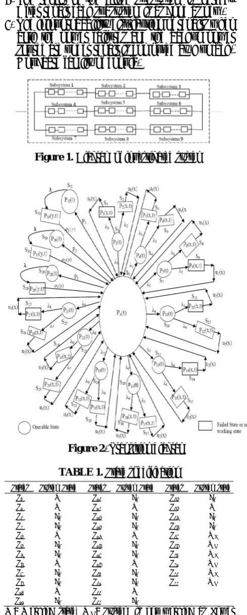
3. We considered the system having nine subsystems arranged in the form of 3x3 matrix in which each row contains three subsystems. The configuration of each row is 2-out-of-3-F, i.e. if any two subsystems fails then the row will fail. The whole system fails if any one row fails.

4. Each subsystem has n units connected in series

(1-out-of-n: F).

5. The system is analyzed with three types of power failures.

6. When the system stops working due to the power failure, a backup power source starts automatically and the system restarts,. Here we assume the backup power source is not very efficient and cannot operate the system for a long period.

7. The repair of the failed subsystem is perfect. After repair each subsystem is as good as new.

8. The joint probability distribution of repairs when both the power failures and the backup power source are under repair is computed by Gumbel -Hougaard family of copula.

Figure 1.Diagram of investigated system

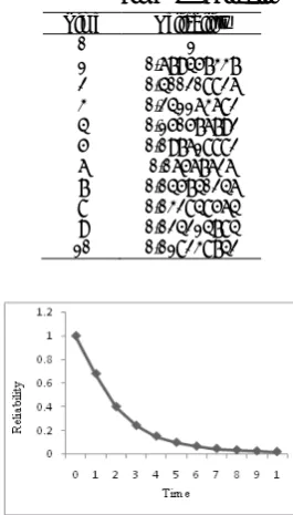
TABLE 1. State specification

States System State States System State States System state

S0 W S12 FR S24 FR

S1 W S13 W S25 W

S2 FR S14 FR S26 FR

S3 FR S15 FR S27 FR

S4 W S16 W S28 WP

S5 FR S17 FR S29 WN

S6 FR S18 FR S30 WP

S7 W S19 W S31 WN

S8 FR S20 FR S32 WP

S9 FR S21 FR S33 WN

S10 W S22 W

S11 FR S23 FR

W: Working state, WN: System is not working as Power failure and standby Power supply under repair, FR: Failed under repair, WP: Working due to standby power supply

(4)

3. NOTATIONS

3 2 1/ /

 : Failure rate of subsystem 1 / subsystem 2 / subsystem 3, where



 



 

 n

k k n

j j n

i i

1 3 1

2 1

1 ,  and 



6 5 4/ /

 : Failure rate of subsystem 4 / subsystem 5 / subsystem 6, where



 



 

 n

r r n

q q n

p p

1 6 1

5 1

4  ,  and 



9 8 7/ /

 : Failure rate of subsystem 7 /

subsystem 8 / subsystem 9, where

, and ,

1 9 1

8 1

7



 



 

 n

g g n

m m n

l

l    

 

where n is the total number of units in each

subsystems 1

P

: Failure rate of blackout.

2

P

: Failure rate of transient fault. 3

P

: Failure rate of Brownout.



: Failure rate of standby power supply.

) (

1 x

u : Repair rate of subsystem 1, subsystem 2 and subsystem 3.

) (

2 x

) (

3 x

) ( 1 y

 : Repair rate of blackout. )

( 2 y

 : Repair rate of transient fault.

) (

3 y

 : Repair rate of brownout.

) (y

v : Repair rate of standby power supply. x: Elapsed repair time.

y: Elapsed repair time for power failure and

standby power supply failure.

Pi(t): Probability that the system is in Sistate at

instant tfor i= 1 to i= 33.

) (s

Pi : Laplace transform of Pi (t).

Pi(x,t): Probability density function that at time t

the system is in failed state Si and the system is under repair, elapsed repair time is x.

Pj(y,t): Probability density function that

at time t the system is not in working

state Sj(j = 29, 31 and 33) and the main power source and standby power source

failure are under repair, elapsed repair time is y.

E p (t): Expected profit during the interval (0, t].

K1, K2: Revenue per unit time and service cost per unit time respectively.

) (x

S : Laplace transform of

S(x)=





 

0 0

)) ( exp(

) (

x

dx x sx

x 



Ifu₁v(y),u₂₁( ),y ₂( ),y ₃( )y then the expression for the joint probability according to Gumbel-Hougaard family of copula is given by

] } )) ( log ( )) ( log {( exp[ ) (

/ 1 2 2

/ 1 1 1

  

 

y y

v y

y y

v y

  

 

  

 

] } )) ( log ( )) ( log {( exp[ )

( 3 1/

3    

 y    v y   y

where θ is the parameter which may take all values

in the interval [1, ∞).

4. FORMULATION OF MATHEMATICAL MODEL

By probability consideration and continuity arguments the following difference-differential equations governing the behavior of the system seems to be good.



      

    

     

0 3 1 0

3 2 1 9 8 7 6

5 4 3 2

1 ₍₎ ₍ ₎ ₍ _, ₎

dx t x P x u t P P P P dt

d

   

    



 



 



0 0

6 1 5

1 0

2

1(x)P(x,t)dx u (x)P(x,t)dx u (x)P(x,t)dx u



 



 



0

11 2 0

9 1 0

8

1(x)P(x,t)dx u (x)P(x,t)dx u (x)P (x,t)dx u



 



 



0 15 2 0

14 2 0

12

2(x)P (x,t)dx u (x)P (x,t)dx u (x)P (x,t)dx u



 



 



0

20 3 0

18 2 0

17



 



 



0 0

24 3 23

3 0

21



 



 



0

29 1 0

27 3 0

26

3(x)P (x,t)dx u (x)P (x,t)dx (x)P (x,t)dx

u 





 

0

33 3 0

31

2(x)P (x,t)dx  (x)P (x,t)dx

(5)

) ( )

( ₁ ₀

1 2

3 P t P t

dt

d _ _ __

    _ _ (2) 0 ) , ( ) ( ₂

1  

  _      t x P x u x t (3) 0 ) , ( ) ( ₃

1  

  _      t x P x u x t (4) ) ( )

( ₂ ₀

4 1

3 P t P t

dt

d _ _ _

     _ _ (5) 0 ) , ( ) ( 5

1  

  _      t x P x u x t (6) 0 ) , ( ) ( ₆

1  

   _      t x P x u x

t (7)

) ( )

( 3 0

7 2

1 P t P t

dt

d _ _ _

   

 _ _ ₍₈₎

0 ) , ( ) ( ₈

1  

  _      t x P x u x

t (9)

0 ) , ( ) ( 9

1  

  _      t x P x u x

t (10)

) ( )

( ₄ ₀

10 6

5 P t P t

dt

d _ _ _

   

 _ _ ₍₁₁₎

0 ) , ( ) ( 11

2  

  _      t x P x u x

t (12)

0 ) , ( ) ( ₁₂

2  

  _      t x P x u x

t (13)

) ( )

( 5 0

13 6

4 P t P t

dt

d _ _ _

   

 _ _ ₍₁₄₎

0 ) , ( ) ( ₁₄

2  

   _      t x P x u x

t (15)

0 ) , ( ) ( ₁₅

2  

  _      t x P x u x

t (16)

) ( )

( 6 0

16 4

5 P t P t

dt

d _ _ _

   

 _ _ ₍₁₇₎

0 ) , ( ) ( ₁₇

2  

  _      t x P x u x

t (18)

0 ) , ( ) ( 18

2  

  _      t x P x u x

t (19)

) ( )

( 7 0

19 9

8 P t P t

dt

d _ _ _

   

 _ _ ₍₂₀₎

0 ) , ( ) ( 20

3  

  _      t x P x u x

t (21)

0 ) , ( ) ( 21

3  

  _      t x P x u x

t (22)

) ( )

( 8 0

22 9

7 P t P t

dt

d _ _ _

   

 _ _ ₍₂₃₎

0 ) , ( ) ( ₂₃

3  

  _      t x P x u x

t (24)

0 ) , ( ) ( 24

3  

  _      t x P x u x

t (25)

) ( )

( ₉ ₀

25 8

7 P t P t

dt

d _ _ _

   

 _ _ ₍₂₆₎

0 ) , ( ) ( 26

3  

  _      t x P x u x

t (27)

0 ) , ( ) ( ₂₇

3  

  _      t x P x u x

t (28)

) ( )

( ₁ ₀

28 t PP t P dt d _   

 __ ₍₂₉₎

0 ) , ( ) ( ₂₉

1  

  _      t y P y x

t  (30)

) ( )

( ₂ ₀

30 t PP t P dt d _   

 __ ₍₃₁₎

0 ) , ( ) ( ₃₁

2  

  _      t y P y x

t  (32)

) ( )

( 3 0

32 t PP t P dt d    

 __ ₍₃₃₎

0 ) , ( ) ( 33

3  

  _      t y P y x

(6)

Boundary conditions: ) ( ) , 0

( ₂ ₁

2 t P t

P  (35)

) ( ) , 0

( ₃ ₁

3 t P t

P  (36)

) ( ) , 0

( ₁ ₄

5 t P t

P  (37)

) ( ) , 0

( ₃ ₄

6 t P t

P  (38)

) ( ) , 0

( ₁ ₇

8 t P t

P  (39)

) ( ) , 0

( ₂ ₇

9 t P t

P  (40)

) ( )

, 0

( ₅ ₁₀

11 t P t

P  (41)

) ( )

, 0

( ₆ ₁₀

12 t P t

P  (42)

) ( )

, 0

( ₄ ₁₃

14 t P t

P  (43)

) ( )

, 0

( ₆ ₁₃

15 t P t

P  (44)

) ( )

, 0

( ₅ ₁₆

17 t P t

P  (45)

) ( )

, 0

( ₄ ₁₆

18 t P t

P  (46)

) ( )

, 0

( ₈ ₁₉

20 t P t

P  (47)

) ( )

, 0

( ₉ ₁₉

21 t P t

P  (48)

) ( )

, 0

( ₇ ₂₂

23 t P t

P  (49)

) ( )

, 0

( ₉ ₂₂

24 t P t

P  (50)

) ( )

, 0

( ₇ ₂₅

26 t P t

P  (51)

) ( )

, 0

( ₈ ₂₅

27 t P t

P  (52)

) ( ) , 0 ( ₂₈

29 t P t

P  (53)

) ( ) , 0 ( ₃₀

31 t P t

P  (54)

) ( ) , 0 ( ₃₂

33 t P t

P  (55) Initial conditions: 1 ) 0 ( 0 

P , and other state probabilities are zero at

t=0. (56)

5. SOLUTION OF THE MODEL

Taking Laplace transformation of (1) to (56) and on further simplification, one can obtain transition state probabilities of the system as:

) ( / 1 ) (

0 s A s

P  (57)

) ( ) ( 0 2 3 1

1 P s

s s P      

 ₍₅₈₎

              s s S s P s s

P ( ) ( ) 1 u1( ) 0 2 3 1 2 2   

 ₍₅₉₎

              s s S s P s s

P ( ) 0( ) 1 u1( ) 2 3 1 3 3     (60) ) ( ) ( 0 1 3 2

4 P s

s s P      

 ₍₆₁₎

              s s S s P s s

P ( ) ( ) 1 u1( ) 0 1 3 2 1 5   

 ₍₆₂₎

              s s S s P s s

P ( ) ( ) 1 u1( ) 0 1 3 2 3 6   

 ₍₆₃₎

) ( ) ( 0 2 1 3

7 P s

s s P      

 ₍₆₄₎

              s s S s P s s

P ( ) 0( ) 1 u1( ) 2 1 3 1 8     (65)               s s S s P s s

P ( ) ( ) 1 u1( ) 0 2 1 3 2 9   

 ₍₆₆₎

) ( ) ( 0 6 5 4

10 P s

s s P      

 ₍₆₇₎

              s s S s P s s

P ( ) ( ) 1 u2( ) 0 6 5 4 5 11     (68)               s s S s P s s

P ( ) ( ) 1 u2( ) 0 6 5 4 6 12   

 ₍₆₉₎

) ( ) ( 0 6 4 5

13 P s

s s P      

 ₍₇₀₎

              s s S s P s s

P ( ) ( ) 1 u2( ) 0 6 4 5 4 14   

 ₍₇₁₎

              s s S s P s s

P ( ) ( ) 1 u2( ) 0 6 4 5 6 15   

 ₍₇₂₎

) ( ) ( 0 4 5 6

16 P s

s s P      

(7)

              s s S s P s s

P ( ) 0( ) 1 u2( ) 4 5 6 5 17     (74)               s s S s P s s

P ( ) ( ) 1 u2( ) 0 4 5 6 4 18   

 ₍₇₅₎

) ( ) ( 0 9 8 7

19 P s

s s P      

 ₍₇₆₎

              s s S s P s s

P ( ) ( ) 1 u3( ) 0 9 8 8 7 20   

 ₍₇₇₎

              s s S s P s s

P ( ) 0( ) 1 u3( ) 9 8 9 7 21     (78) ) ( ) ( 0 9 7 8

22 P s

s s P      

 ₍₇₉₎

              s s S s P s s

P ( ) ( ) 1 u3( ) 0 9 7 8 7 23   

 ₍₈₀₎

              s s S s P s s

P ( ) 0( ) 1 u3( ) 9 7 8 9 24     (81) ) ( ) ( 0 8 7 9

25 P s

s s P      

 ₍₈₂₎

              s s S s P s s

P ( ) ( ) 1 u3( ) 0 8 7 9 7 26   

 ₍₈₃₎

              s s S s P s s

P ( ) ( ) 1 u3( ) 0 8 7 9 8 27   

 ₍₈₄₎

) ( )

( 1 0

28 P s

s P s P   

 (85)

             s s S s P s P s

P ( ) ( ) 1 1( ) 0

1

29 



 ₍₈₆₎

) ( )

( 2 0

30 P s

s P s P   

 (87)

             s s S s P s P s

P ( ) ( ) 1 2( ) 0

2

31 



 ₍₈₈₎

) ( )

( 3 0

32 P s

s P s P   

 (89)

             s s S s P s P s

P33( ) 3 0( ) 1 3( )   (90) where 9 8 7 6 5 4 3 2 1 ( )

(s  s         A       

 ) 1( )

2 3 1 3 3 2

1 S s

s P P P u    

1( ) 1( )

1 3 2 1 2 3 1

2 _S _s

s s S

s   u     u

     

₁( ) ₁( )

2 1 3 1 1 3 2

3 _S _s

s s S

s   u     u

         6 5 4 5 2 1 3

2 ₍ ₎ ₍ ₎

2

1 _ _

              s s S s S

s u u

2( ) 2( )

6 4 5 4 6 5 4

6 _S _s

s s S

s   u     u

        

2( ) 2( )

4 5 6 5 6 4 5

6 _S _s

s s S

s   u     u

        

2( ) 3( )

9 8 8 7 4 5 6

4 _S _s

s s S

s   u     u

        

3( ) 3( )

9 7 8 7 9 8 9

7 _S _s

s s S

s   u     u

        

3( ) 3( )

8 7 9 7 9 7 8

9 _S _s

s s S

s   u     u

         _ _  _   _          s P s S s P s S s u 2 1 8 7 9

8 ₍ ₎ ₍ ₎

1 3

2( ) 3( )

3 _S _s s

P s

S 

  _    (91)

Also up and down state probabilities of the system

are given by

) ( ) ( ) ( ) ( ) ( ) ( )

(s P0 s P1 s P4 s P7 s P10 s P13 s

Pup      

P16(s)P19(s)P22(s)P25(s)P28(s)

P30(s)P32(s)(92)

       ( ) ( ) ( ) ( ) ( ) ( ) )

(s P2 s P3 s P5 s P6 s P8 s P9 s Pdown

P11(s)P12(s)P14(s)P15(s)P17(s) P18(s)P20(s)P21(s)P23(s)P24(s) P26(s)P27(s)P29(s)P31(s)P33(s) (93) From equations (92) and (93), we have

. / 1 ) ( ) ( down

up s P s s

(8)

6. ASYMPTOTIC BEHAVIOUR

Using Able’s lemma

) ( lim )} ( { 0

lim F t

t s F s

s 

 

in equations (92) and (93), one can obtain the following time independent probabilities.

        ) 0 ( 1 ) 0 ( 1 ) 0 ( 1 1 3 2 2 3 1 A A A P_up       6 4 5 6 5 4 2 1 3 ) 0 ( 1 ) 0 ( 1               

 A A

        ) 0 ( 1 ) 0 ( 1 ) 0 ( 1 9 8 7 4 5 6 A A

A  

                  ₁ 8 7 9 9 7 8 ) 0 ( 1 ) 0 ( 1 P A A ) 0 ( 1 ) 0 ( 1 ) 0 (

1 2 3

A P A P

A      

1 1 ) 0 ( 1 ) 0 ( 1 2 3 1 3 2 3 1 2 u u down M A M A

P  

              1 1 ) 0 ( 1 ) 0 ( 1 1 3 2 3 1 3 2 1 u u M A M

A     

           1 1 ) 0 ( 1 ) 0 ( 1 2 1 3 2 2 1 3 1 u u M A M

A     

           2 2 ) 0 ( 1 ) 0 ( 1 6 5 4 6 6 5 4 5 u u M A M

A     

          

2 ₍₀₎ 2

1 ) 0 ( 1 6 4 5 6 6 4 5 4 u M A M

A  u    

           2 2 ) 0 ( 1 ) 0 ( 1 4 5 6 4 4 5 6 5 u u M A M

A     

           3 3 ) 0 ( 1 ) 0 ( 1 9 8 9 7 9 8 8 7 u u M A M

A     

           3 3 ) 0 ( 1 ) 0 ( 1 9 7 8 9 9 7 8 7 u u M A M

A     

           3 3 ) 0 ( 1 ) 0 ( 1 8 7 9 8 8 7 9 7 u u M A M

A     

                 

 2 3

1 2 1 ) 0 ( 1 ) 0 ( 1 P M A P M A P        3 ) 0 ( 1  M A   where ) ( 0 lim ) 0

( A s

s A   , ) ( 1 lim , ) ( 1 lim 2 2 1 1 0 0                       _s s S M s s S M u s u u s u , ) ( 1 lim , ) ( 1 lim 1 1 3

3 ₀ ₀ 

                     _s s S M s s S M s u s u                         s s S M s s S M s s ) ( 1 lim , ) ( 1 lim 3 3 2 2 0 0    

7. PARTICULAR CASES

Distribution In this case the results can be

derived by putting

, ) ( ) ( ) ( , ) ( ) ( ) ( 2 2 1 1 2 1 x u s x u s S x u s x u s

Su u

    , ) ( ) ( ) ( , ) ( ) ( ) ( 1 1 3 3 1 3 y s y s S x u s x u s Su        ) ( ) ( ) ( , ) ( ) ( ) ( 3 3 2 2 3 2 y s y s S y s y s S           (94)

in equations (92) and (93), which yield

         1 3 2 2 3 1 ) ( 1 ) ( 1 ) (       s s B s s B s Pup         6 5 4 2 1 3 ) ( 1 ) ( 1       s s B s s B         4 5 6 6 4 5 ) ( 1 ) ( 1       s s s B s B         9 7 8 9 8 7 ) ( 1 ) ( 1       s s B s s B         ) ( 1 ) ( 1 ) ( 1 ₁ 8 7 9 s B s P s B s s

B   

 ) ( 1 ) ( 1 ₃ 2 s B s P s B s P       2 3 1 3 1 2 3 1 2 ) ( 1 ) ( 1 ) (                        s x u s s B s s Pdown               ) ( 1 ) ( 1 ) ( 1 1 3 2 1

1 x s B s

u s s

B  

  _                  ( ) 1 ) ( 1 1 1 3 2 3

1 x s s u x

u

s  

  _             ) ( 1 ) ( 1 ) ( 1 1 2 1 3 1 x u s s B s s

B  

 

(9)

) ( 1 ) ( 1 ) ( 1 1 2 1 3 2 s B x u s s B

s _

                             6 5 4 6 2 6 5 4 5 ) ( 1         s x u s s ) ( 1 ) ( 1 ) ( 1 6 4 5 4

2 x s B s

u s s

B _   

          6 5

2 4 6 2

1 1 1

( ) ( ) ( )

s u x s B s s u x

        _ _  _ _        

5 6 4 6

5 4 2 5 4

1 1

( ) ( )

s B s s u x s

            _ _   _  _   7 8

2 8 9

1 1 1

( ) ( ) ( )

B s s u x s B s

       _ _        _                  ( ) 1 ) ( 1 3 9 8 9 7

3 x s s u x

u

s  

               ) ( 1 ) ( 1 ) ( 1 3 9 7 8 7 x u s s B s s

B  

  ) ( 1 ) ( 1 ) ( 1 3 9 7 8 9 s B x u s s B

s _

             

7 9 8 9

7 8 3 7 8

1 1

( ) ( )

s s u x s B s

           _ _    _  _   1 2 3 1

1 1 1

( ) ( ) ( )

P P

s u x s B s s y s

         _ _  _ _   _  _    3 2 3

1 1 1 1

( ) ( ) ( ) ( )

P

B s s y s B s s y

         _ _  _{ } _        where 9 8 7 6 5 4 3 2 1 ( )

(s  s        

B          ) ( ) ( ) 1 1 2 3 1 3 3 2 1 x u s x u s P P P    

2 1 1 1 2 1

3 2 1 3 1 1

( ) ( )

u x u x

s s u x s s u x

   

      

     

3 2 1 1 3 1

3 1 1 1 2 1

( ) ( )

u x u x

s s u x s s u x

   

   

     

2 3 1 5 4 2

1 2 1 5 6 2

( ) ( )

u x u x

s s u x s s u x

   

    

     

6 4 2 4 5 2

5 6 2 4 6 2

( ) ( )

u x u x

s s u x s s u x

   

      

     

6 5 2 5 6 2

4 6 2 5 4 2

( ) ( )

u x u x

s s u x s s u x

   

   

     

4 6 2 7 8 3

5 4 2 8 9 3

( ) ( )

u x u x

s s u x s s u x

   

   

     

7 9 3 7 8 3

8 9 3 7 9 3

( ) ( )

u x u x

s s u x s s u x

   

   

     

9 8 3 7 9 3

7 9 3 7 8 3

( ) ( )

u x u x

s s u x s s u x

   

   

     

8 9 3 1 1 2

7 8 3 1

( ) ( )

u x P y P

s s u x s s y s

    

    

     

2 3 3

2 3 ( ) ( ) ( ) ( ) P y y

s y s s y

 



  

  

  

7.2. If Blackout (Total Loss of Power) Occurs Only Up and down state probabilities in this case

can be derived by putting P2= P3= 0 in Equations (92) and (93), which are given by:

) ( 1 ) ( 1 ) ( 1 ) ( 1 3 2 2 3 1 s C s s C s s C s

Pup 

                       ) ( 1 ) ( 1 6 5 4 2 1 3 s C s s C

s  

            ( ) 1 ) ( 1 4 5 6 6 4 5 s C s s C

s  

            ( ) 1 ) ( 1 9 7 8 9 8 7 s C s s C

s  

    ) ( 1 ) ( 1 1 8 7 9 s C s P s C

s      ) ( 1 ) ( 1 ) ( 1 ) ( 1 2 3 1 2 s C s s S s C s s

Pdown u 

                  1

3 1 1 2

3 2 3 1

1 ( ) 1

( )

u S s

s s s C s

         _   _ _   _ _     

1 3 2 1

3 1

1 ( ) 1 1 ( )

( )

u u

S s S s

s s C s s

     _   _    _ _            1

1 3 2 3

1 2 1 2

1 ( ) 1

( )

u S s

s s C s s

         _   _{ }    _{ }    

1 5 4 2

5 6

1 1 ( ) 1 1 ( )

( ) ( )

u u

S s S s

C s s s C s s

     _   _     _ _            2

6 4 4 5

5 6 4 6

1 1 ( ) 1

( ) ( )

u S s

C s s s C s s

             _ _    _ _    

2 6 5 2

4 6

1 ( ) 1 1 ( )

( )

u u

S s S s

s s C s s

            _ _           

5 6 2 4 6

5 4 5 4

1 1 ( )

( )

u

S s

s C s s s

   

 _ 

  _ _

(10)

2 7 8 3

8 9

1 1 ( ) 1 ( ) 1

( ) ( )

u u

S s S s

C s s s s C s

   

 _   _ 

   _ _  

   

   

7 9 3 7 8

8 9 7 9

1 1 ( ) 1

( ) ( )

u S s

s C s s s C s

   

 _ 

    

  _ _  

3 9 8 3

7 9

1 ( ) 1 1 ( )

( )

u u

S s S s

s C s s s

   

 _   _ 

    

 

   

   

3

7 9 8 9

7 8 7 8

1 1 ( ) 1

( ) ( )

u S s

C s s s C s s

   

  

  _ _ 

  __ __  

3 1 1

1 ( ) 1 1 ( )

( )

u P

S s S s

s s C s s

 



     

_ _  _ _



   

   

where

         

( ₁ ₂ ₃ ₄ ₅ ₆ ₇ ₈ ₉

)

(s s         

C

) 1( ) 1( )

2 3

1 2

2 3

1 3

1 S s

s s S s

P u  u

   

  

 

  

 

   

 

 1( ) 1( )

1 3

2 3

1 3

2

1 _S _s

s s S

s u   u

  

 

   



 1( ) 1( )

2 1

3 2

2 1

3

1 _S _s

s s S

s u   u

  

 

   



 2( ) 2( )

6 5

4 6

6 5

4

5 _S _s

s s S

s u   u

  

 

   



 2( ) 2( )

6 4

5 6

6 4

5

4 _S _s

s s S

s u   u

  

 

   



 2( ) 2( )

4 5

6 4

4 5

6

5 _S _s

s s S

s u   u

  

 

   



 3( ) 3( )

9 8

9 7

9 8

8

7 _S _s

s s S

s u   u

  

 

   



 3( ) 3( )

9 7

8 9

9 7

8

7 _S _s

s s S

s u   u

  

 

   



 3( ) 3( )

8 7

9 8

8 7

9

7 _S _s

s s S

s u   u

  

1( )

1 _S _s s

P



 

 

7.3. If Transient Failure (Momentary Loss of Power) Occurs Only Up and down state

probabilities in this case can be derived by putting

P1=P3=0 in Equations (92) and (93).

7.4. If Brownout (Drop in Voltage in an Electrical Power Supply) Occurs Only Up and

down state probabilities in this case can be derived by putting P1=P2=0 in Equations (92) and (93).

8. NUMERICAL COMPUTATION

The Maple software has been used to analyze availability, reliability, M.T.T.F, busy period, cost effectiveness and sensitivity of the system.

8.1. Availability AnalysisTake λ1= 0.1, λ2= 0.1,

λ3= 0.1, λ4= 0.2, λ5= 0.2, λ6= 0.2, λ7= 0.3, λ8= 0.3, λ9= 0.3, P1= 0.4,P2= 0.5, P3= 0.6, λ= 0.7, u1 = u2= u3=ψ1= ψ2= ψ3=φ1= φ2=φ3= v= 1, θ= 1, x = 1 and y = 1. Also, if the repair follows

exponential distribution i.e. Equation (94) holds, then putting all these values in Equation (92) and taking inverse Laplace transformation, we get

-0.009071706019 )

0.6910925727 1.140884736

( ) ( t

up

P t  e 

(-2.038776412 )t _{0.365780518610}-5 ( 0.9984127284 )t

e  e

_{0.00169749090} ( 0.6366204841 )t _{0.02276566549} e

 

_e( 0.4320684754 ) t __{0.00662544791}_e( 0.2318488763 ) t _0.8141359426_e( 2.853201318 ) t

(95) Now, varyingt from 0 to 10 in Equation (95),

we obtain Table 2 and correspondingly Figure 3 representing the behavior of availability of the system with respect to time.

TABLE 2. Time vs. Availability

Time Availibility

0 1

1 0.776014607 2 0.689394547 3 0.671724623 4 0.665228159 5 0.65987168 6 0.65439497 7 0.648753542 8 0.643022658 9 0.637260688 10 0.631504915

(11)

8.2. Reliability Analysis Let us fix failure rates

as λ1= 0.1, λ2= 0.1, λ3= 0.1, λ4= 0.2, λ5= 0.2, λ6= 0.2, λ7= 0.3, λ8= 0.3, λ9= 0.3, P1= 0.4, P2= 0.5, P3 = 0.6, λ= 0.7, repair rates u1=u2=u3= ψ1= ψ2=

ψ3= φ1 = φ2= φ3= v = 0, θ= 1, x = 1 and y = 1. Also, let the repair follows exponential distribution. Now, by putting all these values in Equation (92), using Equation (94) and setting t=

0, 1, 2, 3, 4, 5, 6, 7, 8, 9, 10, one can obtain Table 3 and Figure 4 which represent how reliability varies as the time increases.

8.3. M.T.T.F. Analysis Let us suppose that

repair follows exponential distribution then using equation (94) and from

M.T.T.F. =lim up( )

0P s

s

we have the following four cases:

1.Fixing λ1= 0.1, λ2= 0.1, λ3= 0.1, λ4= 0.2, λ5= 0.2, λ6= 0.2, λ7= 0.3, λ8= 0.3, λ9= 0.3, P2= 0.5, P3= 0.6, λ= 0.7, u1= u2=u3= ψ1= ψ2=

ψ3=φ1= φ2= φ3= v= 0, θ= 1, x= 1 and y= 1 and varying the value of P1as 0.1, 0.2, 0.3, 0.4, 0.5, 0.6, 0.7, 0.8, 0.9, 1.0, one can obtain variation of M.T.T.F. with respect to P1. 2.Let us set λ1= 0.1, λ2= 0.1, λ3= 0.1, λ4= 0.2,

λ5= 0.2, λ6= 0.2, λ7= 0.3, λ8= 0.3, λ9= 0.3, P1 = 0.4, P3= 0.6, λ= 0.7, u1=u2=u3=ψ1= ψ2=

ψ3=φ1= φ2= φ3= v= 0, θ= 1, x= 1 and y= 1 and varying P2as 0.1, 0.2, 0.3, 0.4, 0.5, 0.6, 0.7, 0.8, 0.9, 1.0, one can obtain change of M.T.T.F. with respect to P2.

3. By taking λ1= 0.1, λ2= 0.1, λ3= 0.1, λ4= 0.2,

λ5= 0.2, λ6= 0.2, λ7= 0.3, λ8= 0.3, λ9= 0.3, P1 = 0.4, P2= 0.5, λ= 0.7, u1=u2=u3=ψ1= ψ2=

ψ3=φ1= φ2= φ3= v= 0, θ= 1, x= 1 and y= 1 and varying P3as 0.1, 0.2, 0.3, 0.4, 0.5, 0.6, 0.7, 0.8, 0.9, 1.0, one can obtain variation of M.T.T.F. with respect to P3.

All the three cases described above are depicted by Table 4 and Figure 5.

4.Assume λ1= 0.1, λ2= 0.1, λ3= 0.1, λ4= 0.2, λ5 = 0.2, λ6= 0.2, λ7= 0.3, λ8= 0.3, λ9= 0.3, P1= 0.4, P2= 0.5, P3= 0.6, repairs rates be u1=u2 =u3=ψ1= ψ2= ψ3 =φ1= φ2= φ3= v= 0, θ= 1, x= 1 and y= 1 and increase the value of λ

from 0.1 to 1.0, we obtain Table 5 and Figure 6 which represents the manner in which

M.T.T.F. varies with respect to λ.

TABLE 4. Power supply failure (Pi) vs. M.T.T.F.

where i = 1 (Blackout), i = 2 (Transient) and i = 3 (Brownout)

P1 M.T.T.F. P2 M.T.T.F. P2 M.T.T.F.

0.1 2.404761905 0.1 2.438423645 0.1 2.474489796 0.2 2.373271889 0.2 2.404761904 0.2 2.438423645 0.3 2.34375 0.3 2.373271889 0.3 2.404761904 0.4 2.316017316 0.4 2.34375 0.4 2.373271889 0.5 2.289915966 0.5 2.316017316 0.5 2.34375 0.6 2.265306122 0.6 2.289915966 0.6 2.316017316 0.7 2.242063492 0.7 2.265306122 0.7 2.289915966 0.8 2.22007722 0.8 2.242063492 0.8 2.265306122 0.9 2.19924812 0.9 2.2007722 0.9 2.242063492 1 2.179487179 1 2.19924812 1 2.2007722

Figure 5.Power supply failure (Pi) vs. M.T.T.F. where i = 1

(Blackout), i = 2 (Transient) and i = 3 (Brownout )

TABLE 3. Time vs. Reliability

Time Reliability

0 1

1 0.679457337 2 0.400208826 3 0.241163682 4 0.150576792 5 0.097618882 6 0.06567626 7 0.045740246 8 0.032848564 9 0.024214784 10 0.018238742

(12)

8.4. Busy Period Analysis Let the equation (94)

holds then Mean time to repair (M.T.T.R.) of the system is given by

M.T.T.R.lims0Pdown(s)

1. Letting λ1= 0.1, λ2= 0.1, λ3= 0.1, λ4= 0.2, λ5= 0.2, λ6= 0.2, λ7= 0.3, λ8= 0.3, λ9= 0.3, P2= 0.5,

P3= 0.6, λ= 0.7, u1=u2=u3=ψ1= ψ2= ψ3=φ1

= φ2= φ3 = v = 1, θ = 1, x = 1 and y = 1 and varying P1 as 0.1, 0.2, 0.3, 0.4, 0.5, 0.6, 0.7, 0.8, 0.9, 0.1, we obtain the changes of busy period with respect to P1.

2. Taking the values λ1= 0.1, λ2= 0.1, λ3= 0.1, λ4 = 0.2, λ5= 0.2, λ6= 0.2, λ7= 0.3, λ8= 0.3, λ9= 0.3, P1= 0.4, P3= 0.6, λ= 0.7, u1=u2=u3=ψ1

= ψ2= ψ3=φ1= φ2= φ3= v= 1, θ= 1,x= 1, y= 1 and varying P2= 0.1, 0.2, 0.3, 0.4, 0.5, 0.6, 0.7, 0.8, 0.9, 1.0, one can observe how the busy period changes with respect to P2.

3. Varying P3= 0.1, 0.2, 0.3, 0.4, 0.5, 0.6, 0.7, 0.8, 0.9, 1.0, and keeping other parameter fixed at λ1 = 0.1, λ2= 0.1, λ3= 0.1, λ4= 0.2, λ5= 0.2, λ6= 0.2, λ7= 0.3, λ8= 0.3, λ9= 0.3, P1= 0.4, P2= 0.5, λ= 0.7, u1=u2=u3=ψ1= ψ2= ψ3=φ1= φ2

= φ3= v= 1, θ= 1, x= 1,y= 1, one can get the variation of busy period with respect to P3. Variations of busy period with respect to P1,P2

and P3 in the cases (1), (2) and (3) have been shown by Table 6 and Figure 7.

8.5. Sensitivity Analysis Assuming that Equation

(94) holds, we first perform a sensitivity analysis for changes in R(t) resulting from changes in system parameters P1, P2, P3and λ.

Putting λ1= 0.1, λ2= 0.1, λ3= 0.1, λ4= 0.2, λ5= 0.2,

λ6= 0.2, λ7= 0.3, λ8= 0.3, λ9= 0.3, P2= 0.5, P3= 0.6, λ= 0.7, u1=u2=u3=ψ1= ψ2= ψ3= φ1= φ2=

φ3= v= 0, θ= 1, x= 1 and y= 1 in Equation (92), and then differentiating with respect to P1, we get:

          

2 1 2

1

1 ( .2)( 2.9 )

3 . )

9 . 2 (

1 )

(

P s

s P s

P s R

₂

1 2

1 ( .6)( 2.9 )

9 . )

9 . 2 ( ) 4 . (

6 .

P s

s P s

s      

₂

1 1

1) ( .7)( 2.9 )

9 . 2 ( ) 7 . (

1

P s

s

P P

s

s      



₂

1)

9 . 2 ( ) 7 . (

1 . 1

P s

s  



TABLE 6. Power failure (Pi) vs. Busy Period where

i = 1(Blackout), i = 2 (Transient) and i = 3 (Brownout)

Busy Period w.r.t. Blackout Transient Brownout

0.1 29.1 28.1 27.1 0.2 29.2 28.2 27.2 0.3 29.3 28.3 27.3 0.4 29.4 28.4 27.4 0.5 29.5 28.5 27.5 0.6 29.6 28.6 27.6 0.7 29.7 28.7 27.7 0.8 29.8 28.8 27.8 0.9 29.9 28.9 27.9 1 30 29 28

Figure 7.Power failure (Pi) vs. Busy Period where

i = 1(Blackout), i = 2 (Transient) and i = 3 (Brownout)

TABLE 5. Standby power supply

failure (λ) vs. M.T.T.F.

λ M.T.T.F 0.1 6.212121212 0.2 3.93939393939 0.3 3.181818182 0.4 2.803030303 0.5 2.575757576 0.6 2.424242424 0.7 2.316017316 0.8 2.234848485 0.9 2.171717171 1 2.121212121

Figure 6.Standby power supply failure (λ) vs. MTTF

(13)

Taking inverse Laplace transformation gives:

400000 . 2 ) 5 11 ( 50000000 .

27 ) (

2 1

) 0 700000000 . 0 (

1

 

 

 

P e

P t

R t



 



 

2 1

) 2000000000 .

0 (

2 1

) 4000000000 .

0 (

) 10 27 ( 30 )

2 5 ( 000

P e

P

e t t

(0.1000000000(52P₁)(115P₁)(2310 P₁)(2710P₁)(7000P₁348300P₁211100

90 82797) 700000 6 0.9660000

1

1 t P 

P

107P150.55231000108P140.1673316

0010 0.28304245010 2 0.253

1 9 3

1

9_P _ _P _

119174109P₁0.9333895890108)

2

1 )

) 10 29 ( 1000000000 .

0

( 1 _/((₁₁ ₅_P₎

e  P t 

(2310P₁)2(52P₁)2(2710P₁)2)

₂

1 ) 6000000000 .

0 (

) 10 23 ( 90

P

e t



 

Using the same procedure described above, we can get (), ()and ().

3

2 

 

 R t

P t R P

t R

Now, we perform a sensitivity analysis of changes in M.T.T.F. with respect to P1, P2, P3 and

λ. Setting λ1= 0.1, λ2= 0.1, λ3= 0.1, λ4= 0.2, λ5= 0.2, λ6= 0.2, λ7= 0.3, λ8= 0.3, λ9= 0.3, P2= 0.5, P3 = 0.6, λ= 0.7, u1=u2=u3=ψ1= ψ2= ψ3=φ1= φ2=

φ3= v= 0, θ= 1, x= 1 and y= 1 in Equation (92) then using Equation (94), we get:

1 1

10 29

20 99 7142857143 .

0 . . . .

P P F

T T M

  

Differentiating it with respect to P1, we have:

1

1 29 10

1 28571429 .

14 . . . .

P P

F T T M

 

 

₂

1 1

) 10 29 (

) 20 99 ( 142857143 .

7

P P 

 

Using the same procedure

2

. . . .

M T T F P 

 ,

3

. . . .

and

M T T F M T T F

P 

 

  can be obtained.

Numerical results of the sensitivity analysis for the system reliability and the M.T.T.F. are presented in Figures 8 - 11 and Tables 7-10.

TABLE 7. Sensitivity of system reliability w. r. t. Piwhere i=1 (Blackout), i=2 (Transient) and i=3

(Brownout)

1

( )

R t P



 ₂

( )

R t P



 3

( )

R t P

 

Time

0 0 0 0

1 -0.036564414 -0.035039093 -0.028560154 2 -0.033135699 -0.0314714 -0.024744067 3 -0.025842503 -0.024514741 -0.019190421 4 -0.019602452 -0.018589659 -0.014535014 5 -0.01473436 -0.013971798 -0.010920474 6 -0.011069977 -0.010497208 -0.008205377 7 -0.008353782 -0.007922136 -0.006194561 8 -0.006348868 -0.006021452 -0.004710522 9 -0.004865326 -0.004614962 -0.003612083 10 -0.003760494 -0.003567407 -0.0027936

Figure 8.Sensitivity of system reliability w. r. t. Pi

where i = 1 (Blackout), i = 2 (Transient) and i = 3 (Brownout)

TABLE 8. Sensitivity of system reliability w.r.t.

standby power supply failure (λ)

( )

R t



 

Time λ=0.2 λ=0.5

0 0 0

1 -0.274123478 -0.215938461 2 -0.544280636 -0.324031722 3 -0.711007298 -0.315920924 4 -0.799534658 -0.26411302 5 -0.832609568 -0.204165507 6 -0.827422185 -0.150504276 7 -0.7967571 -0.107462627 8 -0.750021404 -0.074991328 9 -0.694048922 -0.051435788 10 -0.633724011 -0.034806997