SIMULTANEOUS DUE DATE ASSIGNMENT
AND
LOT SIZING WITH UNCERTAIN FLOW TIMES
G. Mokhtari* and F. Kianfar
Department of Industrial Engineering, Sharif University of Technology Tehran, Iran
[email protected] - [email protected] *Corresponding Author
(Received: January 31, 2007 – Accepted in Revised Form: September 13, 2007)
Abstract Due date assignment for customer orders has been studied in various production environments using different modeling approaches. In this paper the researchers consider a production system in which the orders of several customers are produced in a single batch because of the economy of scale. If a batch is completed before receiving customer orders, inventory carrying cost is incurred but if it is completed after receiving customer orders, shortage cost is incurred and finally if the order is delivered after its due date, tardiness cost is charged. The problem is to decide on batch size, due date of batch (imposed on supply process) and lead time (to be quoted to the next coming customers) so that relevant costs are minimized. The objective function is to minimize total cost of supply, inventory carrying, shortage and tardiness. Production flow times are probabilistic which follow a probability distribution. The proposed model is solved using real-coded genetic algorithms and numerical results are presented. This work was motivated by a heavy equipment production system which has some products with relatively low demand rates, high prices and long supply lead times.
Keywords Due Date Assignment, Lot-Sizing, Lead Time Quotation, Real-Coded Genetic Algorithms
ﻩﺪﻴﻜﭼ
ﺎـﺑﻭﻒـﻠﺘﺨﻣﯼﺪﻴﻟﻮﺗﯼﺎﻫﻂﻴﺤﻣﺭﺩﻥﺎﻳﺮﺘﺸﻣﺵﺭﺎﻔﺳﻞﻳﻮﺤﺗﺪﻋﻮﻣﻦﻴﻴﻌﺗﺩﺭﻮﻣﺭﺩ
ﺵﻭﺭﺯﺍﻩﺩﺎﻔﺘـﺳﺍ
ﻝﺪﻣﯼﺎﻫ
ﺖﺳﺍﻩﺪﺷﻖﻴﻘﺤﺗ،ﯽﺗﻭﺎﻔﺘﻣﯼﺯﺎﺳ
.
ﻪﻟﺎﻘﻣﻦﻳﺍﺭﺩ ،
ﯽﻣﺮﻈﻧﺭﺩﺍﺭﯼﺪﻴﻟﻮﺗﻢﺘﺴﻴﺳﮏﻳ
ﻞـﻴﻟﺩﻪـﺑﻪـﮐﻢﻳﺮﻴﮔ
ﭻﺑﮏﻳﺭﺩﯼﺮﺘﺸﻣﻦﻳﺪﻨﭼﺵﺭﺎﻔﺳ،ﺱﺎﻴﻘﻣﺯﺍﯽﺷﺎﻧﯽﻳﻮﺟﻪﻓﺮﺻ
، ﯽﻣﺪﻴﻟﻮﺗ ﺪﻧﻮﺷ
. ﺖـﻓﺎﻳﺭﺩﺯﺍﻞﺒﻗ،ﭻﺑﺪﻴﻟﻮﺗﺮﮔﺍ
ﺑﯼﺩﻮﺟﻮﻣﯼﺭﺍﺪﻬﮕﻧﻪﻨﻳﺰﻫ،ﺪﺑﺎﻳﻥﺎﻳﺎﭘﻥﺎﻳﺮﺘﺸﻣﺵﺭﺎﻔﺳ ﯽﻣﺩﻮﺟﻮ
ﻥﺎﻳﺮﺘﺸـﻣﺵﺭﺎﻔـﺳﺖـﻓﺎﻳﺭﺩﺯﺍﺪـﻌﺑﺮﮔﺍﺎﻣﺍﺪﻳﺁ
ﻞـﻳﻮﺤﺗﯼﺮﺘﺸـﻣﻪﺑ،ﻩﺪﺷﻦﻴﻴﻌﺗﺪﻋﻮﻣﺯﺍﺪﻌﺑﯽﺷﺭﺎﻔﺳﺮﮔﺍﺖﻳﺎﻬﻧﺭﺩﻭﺖﺷﺍﺩﻢﻴﻫﺍﻮﺧﺩﻮﺒﻤﮐﻪﻨﻳﺰﻫ،ﺩﻮﺷﻞﻴﻤﮑﺗ
ﯽﻣﺩﺎﺠﻳﺍﺮﻴﺧﺄﺗﻪﻨﻳﺰﻫ،ﺩﻮﺷﻩﺩﺍﺩ ﺩﺩﺮﮔ
. ﭻـﺑﻞﻳﻮﺤﺗﺪﻋﻮﻣ،ﭻﺑﻩﺯﺍﺪﻧﺍﺩﺭﻮﻣﺭﺩﯼﺮﻴﮔﻢﻴﻤﺼﺗﺯﺍﺖﺳﺍﺕﺭﺎﺒﻋﻪﻠﺌﺴﻣ
)
ﺮﺑﻩﺪﺷﻝﺎﻤﻋﺍ ﺗﺪﻨﻳﺍﺮﻓ
ﺄ ﻦﻴﻣ
(
ﻞﻳﻮﺤﺗﺕﺪﻣﻭ
)
ﯽﻣﻡﻼﻋﺍﻥﺎﻳﺮﺘﺸﻣﻪﺑﻪﮐ ﺩﺩﺮﮔ
( ﻪـﮐﯼﻮـﺤﻧﻪﺑ، ﻉﻮـﻤﺠﻣ
ﺎـﻫﻪـﻨﻳﺰﻫ
ﺩﺩﺮﮔﻞﻗﺍﺪﺣ
.
ﺗﯼﺎﻫﻪﻨﻳﺰﻫﻞﮐﯼﺯﺎﺳﻞﻗﺍﺪﺣ،ﻑﺪﻫﻊﺑﺎﺗ ﺄ
ﺖـﺳﺍﺮﻴﺧﺄـﺗﻭﺩﻮﺒﻤﮐ،ﯼﺩﻮﺟﻮﻣﯼﺭﺍﺪﻬﮕﻧ،ﻦﻴﻣ
. ﻥﺎـﻣﺯ
ﯽﻣﯼﻭﺮﻴﭘﯽﻟﺎﻤﺘﺣﺍﻊﻳﺯﻮﺗﮏﻳﺯﺍﻭﻩﺩﻮﺑﯽﻟﺎﻤﺘﺣﺍ،ﺪﻴﻟﻮﺗﻥﺎﻳﺮﺟﯼﺎﻫ ﺪﻨﻨﮐ
.
ﺪﺷﻪﺋﺍﺭﺍﻝﺪﻣ
ﻢﺘﻳﺭﻮـﮕﻟﺍﺯﺍﻩﺩﺎﻔﺘﺳﺍﺎﺑ،ﻩ
ﺪـﻧﺍﻩﺪـﺷﻪﺋﺍﺭﺍﯼﺩﺪﻋﺞﻳﺎﺘﻧﻭﻩﺪﺷﻞﺣ،ﯽﻘﻴﻘﺣﮓﻨﻳﺪﮐﺎﺑﮏﻴﺘﻧﮊ
. ﺪـﻴﻟﻮﺗﻢﺘﺴـﻴﺳﮏـﻳﺱﺎـﺳﺍﺮـﺑﻖـﻴﻘﺤﺗﻦـﻳﺍ
ًﺎﺘﺒﺴﻧﯼﺎﺿﺎﻘﺗﺎﺑﻝﻮﺼﺤﻣﯼﺩﺍﺪﻌﺗﻪﮐﺖﻓﺮﮔﻡﺎﺠﻧﺍﻦﻴﮕﻨﺳﺕﺍﺰﻴﻬﺠﺗ
ﺪـﻴﻟﻮﺗ،ﯽﻧﻻﻮﻃﻦﻴﻣﺄﺗﺕﺪﻣﻭﻻﺎﺑﺖﻤﻴﻗ،ﻢﮐ
ﯽﻣ ﺪﻳﺎﻤﻧ
.
1. INTRODUCTION
In make-to-order production systems, it is crucial to have short lead times and a good due date performance. With the latter it is meant that orders are delivered as close as possible to their due dates. Researches have shown that price, quality and response time are the most important criteria in
contractors selection. Hence trying to reduce lead times and on time delivery is essential for competition.
the order close to the order due date. On the other hand long lead times make it easy for the order realization function to obtain a good due date performance but these lead times are, in general, not acceptable for the customers. Long lead times not only dissatisfy customers but also increase WIP and total inventories. Many authors have studied this trade-off between the length of lead times quoted to the customer and the delivery reliability. In due date assignment two kinds of costs exist:
• Too long lead time costs (lost sales, lower prices, customer dissatisfaction,…)
• Too short lead time costs (Tardiness penalties, more production costs, quality problems, customer dissatisfaction,…) Due dates must be set so as to minimize total costs. In other words, due dates must be attractive for customers and profitable for manufacturers.
The majority of published papers about due date assignment assume a make-to-order production system in which each customer order is quoted and processed separately. The researcher’s contribution is formulating and solving due date assignment in a make-to-demand production system in which the order of several customers are aggregated and produced in a single batch.
The rest of this paper is organized as follows. In Section 2, some of the relevant literature is summerized while Section 3 presents this paper’s analytical model. In Section 3, the specific problem is described and modeled. In Section 4 real-coded genetic algorithms are applied to solve the sample problems and analyze the results.
2. LITERATURE REVIEW
In this paper a problem is considered which is simultaneously related to due date assignment and lot sizing literature. Hence the principal research streams in these distinct areas are reviewed. Sections 2.1, 2.2 are about due date assignment and lot sizing respectively.
2.1. Due Date Assignment Literature
There are many published papers about due dateassignment problem. Here three principal research streams are recognized:
• Studies that combine due date assignment with orders sequencing and scheduling problems [13,15,22,36]. In this line of research, production systems may include single machines, parallel machines, job shop, flow shop or continuous. • Studies that use a simulation approach to estimate order lead time based on some independent variables [12].
• Studies that use flow time approach for due date assignment. In this approach, each order has a flow time which usually has a probability distribution function. [23,28]
Key factors that differentiate between the above streams are:
• Amount and precision of information considered about workshop schedule and new arriving orders: When due date assignment is mixed with scheduling, very detailed information about workshop load (jobs already in system) is considered. But when flow time approach is used, information about workshop load is considered with some approximations. Some empirical methods use non-stochastic estimates like total work content (TWK), total work on the critical path (TWKCP), job processing time plus a slack (SLK), the number of operations (NOP), processing time and current queue length (JIQ), job processing time, waiting time and number of jobs in the system (JIS).
• Decision variables : may include optimal due date, product price [16], order acceptance … • Objective function: may be minimizing costs (including tardiness and earliness cost, long quoted lead time cost) or maximizing profit (when decision has an effect on sales revenue
The flow time approach is followed in this paper so papers that are in this line of research are concentrated on.
distribution function. Late deliveries incur two kinds of tardiness costs (independent of tardiness time and proportional to the amount of tardiness). The objective function is maximizing profit which is revenue minus lead time related costs. Optimal lead time is obtained by derivation. Finally they study the model performance using a simulation model. Ooijen and Bertrand [23] follow the approach of Bertrand and Ooijen [28]. In this paper they try to use new order information and work loads are taken into account. They define Internal and external due dates. Internal due dates are used for determining the priorities on the shop floor and external due dates are quoted to the customer. Internal due date is a function of arrival time of order, number of operations of order, processing time of operations, number of orders in the shop at the arrival time of order, number of machines in the shop and steady state utilization. At the end of the paper they use simulation to verify model performance.
Song, et al [11] investigates the problem of assigning product due dates for complex multistage assemblies. Manufacturing and assembly processing times are stochastic. In order to analyze multistage assemblies their product structures are decomposed into stage subsystems. A two-stage assembly system has some components that are processed in parallel and then assembled. In assigning product due dates it is assumed that there is a production plan of start times which is being followed. An operation begins at its planned start time, unless it is delayed. It would then start immediately after the completion of previous activities, or in the case of assemblies, when all components are available. The completion time of a component and first stage is obtained based on these assumptions. They use three different forms of earliness and tardiness cost functions (absolute deviation, squared deviation and linear combination of positive and negative deviations).
Saibal and Jewkes [39] study due date assignment when both demand rate and product price are lead time sensitive. Orders arrive according to a Poisson process and processing times are exponentially distributed. The firm’s objective is to maximize profits by selecting an optimal guaranteed delivery time taking into account that (i) reducing delivery time will require investment, and (ii) the firm must be able to satisfy a pre-specified service level. Mean demand rate is
modeled as a decreasing linear function of price and delivery time while price itself is a decreasing linear function of the guaranteed delivery time. Hence demand rate is a function of delivery time. They assume that the investment function takes a linear form and later discuss the extension to non-linear investment functions. The firm has a unit operating cost, initially assumed to be constant (i.e., economies of scale do not exist).
Veral [12] uses a simulation model for estimating the order flow time which is the base of due date assignment. An average allowance for operation i at machine j is calculated using the processing time of operation i at machine j and average utilization of machine j. The flow allowance for a job is calculated as the sum of all its operations.
2.2. Lot Sizing Literature
The concept of batching has been examined in various families of problems. Two major families of problems are lot sizing and lot scheduling problems. For a review of lot sizing problems the reader is referred to [52]. Lot sizing problems are production planning problems with setups between production lots. Because of these setups, it is often too costly to produce a given product in every period. On the other hand, generating fewer setups by producing large quantities to satisfy future demands, results in high inventory holding costs. Thus, the objective is to determine the periods where production should take place, and the quantities to be produced, in order to satisfy demand while minimizing production, setup and inventory holding costs. Other costs might also be considered. Examples are backorder cost, changeover cost, etc. Several models have been proposed for lot sizing problems. One of the ancestors of these models is the Economic Order Quantity (EOQ) model, which is a continuous time model with an infinite time horizon. It considers a single item and imposes no capacity restrictions. Later, the EOQ model was extended to consider multiple items and capacity limits. Research on continuous models is still carried out.The classification of lot sizing problems is based on several criteria: number of machines, number of production stages (levels), capacity constraints and their nature (fixed or variable), length of production periods, etc. Based on production stages, single-level and multi-level problems can be considered. While if the focus is on period length, big time bucket problems and small time bucket problems can be considered. Small time bucket problems have short production periods, which normally are of the order of a few hours. Big time bucket problems consist of longer time periods, normally of the order of a few days or weeks. The latter can be seen as a time aggregation of the former. This leads to the consideration of hierarchical planning problems. Lot sizing problem may be considered capacitated or uncapacitated. The latter can be seen as a lot sizing problem with a single (or aggregate) product, in which the production capacity is assumed to be high enough to never be binding in an optimal solution.
For a review of lot scheduling problems the reader is referred to [7,9]. In lot scheduling problems jobs may be batched if they share the same setup on a machine or a machine can process several jobs simultaneously. In these problems, doing jobs in batches has fewer costs than doing them separately.
One situation where benefits may result from batching occurs when machines require setups if they are to process jobs that have differing characteristics. The setup may reflect the need to change a tool or to clean the machine. In a family scheduling model, jobs are partitioned into families according to their similarity, so that no setup is required for a job if it belongs to the same family of the previously processed job. However, a setup time is required at the start of the schedule and on each occasion when the machine switches from processing jobs in one family to jobs in another family. In this model, a batch is a maximal set of jobs that are scheduled contiguously on a machine and share a setup. Large batches have the advantage of high machine utilization because the number of setups is small. On the other hand, processing a large batch may delay the processing of an important job belonging to a different family.
In lot scheduling, problems involving the
scheduling of a single machine, of m parallel machines, and of m-machine flow shops, job shops and open shops may be considered. There is a set of jobs to be processed. The processing time of jobs, release dates, due dates and the weights of jobs is known.
In scheduling problems it is often assumed that due dates are determined before and some of them in which due date is a part of decision variables, the problem and costs structure is different from due date assignment problem [see References 20, 21].
3. PROBLEM DESCRIPTION AND FORMULATION
In this section, a specific problem is formulated with flow time approach. The problem was defined in a heavy equipments company. Consider a product that has deterministic demand and because of economy of scale is produced in batches and each batch satisfies several customer orders. Because of relatively long lead times, supply of a batch usually starts based on demand forecasting. If a batch is completed before receiving customer orders for it, inventory carrying cost is incurred but if it is completed after receiving customer orders, a due date is quoted to each customer and a shortage cost is charged (which is also called backlogging cost in inventory systems literature and reveals in the forms of sales price reduction, customer goodwill …). If an order is delivered after its due date, tardiness cost is incurred.
To formulate the problem symbolically, some definitions and notations will be required. Consider a product with an interval time between two successive orders of λ. After receiving each order, a due date is quoted to its customer, if it could not be delivered simultaneously. Let L(i) be function which determines the lead time quoted to customer i. Due date of order i will be iλ+L(i) since order i is received at iλ. Quoting a lead time x to a customer, will charge w.x cost. Supply cost function is S(Q) in which Q is the batch size. Let
1
cost rate per unit of product. Inventory carrying cost per unit per unit time is h. Consider d to be the batch due date that is used in supply planning process. Because of uncertainty in supply process, batch completion time is a random variable (showed by Xd) with a probability density function f which is a function of the batch due date. In other words, if the supply due date of a batch is set at d, the batch completion time will be a random function of d. So decision variables are:
• Batch size (Q) • Batch due date (d)
• Customer due date assignment function, L(i) • If the batch size is Q, shortage cost of a
cycle will be
∑
= > λ
Q 1 i ) i d X ( P ). i ( L
w (1)
In which Xd is batch receive time and P(Xd >iλ) is the probability that the batch is not received until order receiving time, iλ.
Inventory carrying cost is incurred for products that are not sold until batch completion. Inventory carrying cost of a cycle will be
⎥ ⎥ ⎦ ⎤
∫ λ∞− λ−
∑ = ⎢⎢⎣
⎡
+
∫λλ+ λ+ −
i (x)dx
d X f ). x i ( Q 1 i ) i ( L i
i (x)dx
d X f ). x ) i ( L i ( h (2)
Where iλ+L(i)−x is the duration of holding product i when supply completion time is x and the product due date is iλ+L(i). Inventory carrying cost expression has two parts because it could happen to be in two different situations. Firstly, it incurs if the batch is received before customer order, iλ. Secondly, it happens if the product is not received before customer order so a lead time is quoted to him, but it is received before due date quoted to its customer.
Tardiness cost occurs for products that are delivered beyond their assigned due date.
Tardiness cost of a cycle will be
∑
= ∫∞ +λ − λ−
π + ∑
= > λ+
π
Q
1
i i L(i)
dx ) x ( d X f )]. i ( L i x [ 2 Q 1
i P[Xd i L(i)] 1
(3)
Where P[Xd >iλ+L(i)] is the probability of tardiness and [x−iλ−L(i)]is tardiness of product i, if batch is received at time x. It is obvious that tardiness occurs when the batch is received in range
[
iλ+L(i),∞]
.Hence total cost of a cycle is
+
=S(Q)
) Q (
Z ∑
= > λ
Q 1 i ) i d X ( P ). i ( L w + ⎥ ⎦ ⎤
∫ λ∞− λ−
∑
= ⎢⎣
⎡
+
∫ +λλ λ+ −
i (x)dx
d X f ). x i ( Q 1 i ) i ( L i
i (i L(i) x).fXd(x)dx h
+
∑
= ∫∞ +λ − λ−
π + ∑
= > λ+
π
Q 1
i i L(i)[x i L(i)].fXd(x)dx 2
Q 1
i P[Xd i L(i)] 1
(4)
Average cost of unit product is Z(Q) Q
1 which must be minimized.
For further elaboration of the model, L(i) is considered to be a linear function of i, i.e.
ib a ) i (
L = − . Although with respect to the proposed solution method, there is no limitation in considering other structures for function L(i). Parameters a, b together with d and Q are the decision variables of the model.
4. MODEL SOLUTION USING GENETIC ALGORITHMS
own level of “fitness”. The change in the population is achieved by the selection, reproduction and mutation procedures within the method. The operation of these three procedures is dependent upon the fitness of the individuals concerned.
Every good GA needs to balance the extent of exploration of information obtained up until the current generation through recombination and mutation operators with the extent of exploitation through the selection operator. If the solutions obtained are exploited too much, premature convergence is expected. On the other hand, if too much stress is given on a search (i.e. exploration), the information obtained thus far has not been used properly. Therefore, the solution time may be enormous and the search exhibits a similar behavior to that of a random search. The issue of exploration and exploitation makes a recombination and mutation operator dependent on the chosen selection operator for successful GA run.
4.1. Encoding
Genetic algorithms are characterized by the fact that all the information for any individual in the population is encoded using some linear encoding system. This (usually binary) encoding is intended to be analogous to natural DNA consisting of a string of four kinds of chromosomes. The standard encoding technique for applying genetic algorithms to non-linear optimization problems (where the parameters are continuous and real), is a concatenation of all the binary approximations to each number. Handling continuous search space with binary coded genetic algorithm has several difficulties [40]. Real coded genetic algorithm represents parameters without coding, which makes representation of the solutions very close to the natural formulation of many problems. Then a chromosome is a vector of floating point numbers, the precision of which will be restricted to that of the computer with which the algorithm is carried out. The size of the chromosomes is kept the same as the length of the vector which is the solution to the problem; in this way, each gene represents a variable of the problem. The values of the chromosome genes are forced to remain in the interval established by the variables they represent so the genetic operators must observe this requirement. In real coded GA (RCGA) recombination and mutation operators aredesigned to work with real parameters. In this paper, RCGA is applied for optimization.
4.2. Cross-Over
The means by which two different chromosomes (i.e. members of the population) can combine to form some new “offspring” is cross-over. Here, some well-known or recently proposed crossover operators are presented and considered in experiments.
4.2.1. Blend crossover (BLX-α) [46] Assume that C1=(c11,...,c1n) and C2=(c12,...,c2n)are two chromosomes that have been selected to apply the crossover operator to them. An offspring,H=(h1,...,hi,...,hn) is generated, where hi is a randomly (uniformly) chosen number of the interval [cmin − .Iα,cmax+ .Iα],
) 2 i c , 1 i c max( max
c = , cmin =min(c1i,ci2),
min c max c
I= − . The BLX-0.0 and BLX-0.25 are also called flat crossover and extended intermediate crossover respectively.
4.2.2. Heuristic crossover (HX) [49] With this operator, also called direction based crossover, from a pair of parents x(1)=(x1(1),x2(1),...,xn(1)) and x(2)=(x1(2),x2(2),...,xn(2)) an offspring
) n y ,..., 2 y , 1 y (
y= is generated in the following manner:
) 2 ( i x ) ) 1 ( i x ) 2 ( i x ( u i
y = − +
Where u is a uniformly distributed random number in the interval [0,1] and the parent x(2) has a fitness value no worse than that of parent x(1). If the offspring generated lies outside the feasible region, a new random number u is generated to produce another offspring. If required, this process is repeated up to k times. If it fails to produce a feasible offspring, like laplace operator, a random point in the feasible region is chosen. In this paper k is fixed to be 4 (as in [50,45]).
4.2.3. Laplace crossover (LX) [45] Laplace crossover is based on laplace distribution. Distribution function of Laplace distribution is given by ⎪ ⎪ ⎪ ⎩ ⎪⎪ ⎪ ⎨ ⎧ > − − − ≤ − = a x , b a x e 2 1 1 a x , b a x e 2 1 ) x (
F (5)
Where a∈Ris called the location parameter and b > 0 is termed as scale parameter.
Using laplace crossover, two offspring
) ) 1 ( n y ,..., ) 1 ( 2 y , ) 1 ( 1 y ( ) 1 (
y = and
) ) 2 ( n y ,..., ) 2 ( 2 y , ) 2 ( 1 y ( ) 2 (
y = are generated from a
pair of parents x(1)=(x1(1),x2(1),...,xn(1)) and
) ) 2 ( n x ,..., ) 2 ( 2 x , ) 2 ( 1 x ( ) 2 (
x = in the following way.
First, a uniformly distributed random number
[ ]
0,1u∈ is generated. Then, a random number β is generated which folalows the laplace distribution by simply inverting the distribution function of Laplace distribution as follows:
⎪ ⎩ ⎪ ⎨ ⎧ > + ≤ − = β 2 1 u , ) u ( Ln . b a 2 1 u , ) u ( Ln . b a (6)
The offspring are given by the equations
) 2 ( i x ) 1 ( i x ) 2 ( i x ) 2 ( i y ) 2 ( i x ) 1 ( i x ) 1 ( i x ) 1 ( i y − β + = − β + =
From the above equations it is clear that both the offspring are placed symmetrically with respect to the position of the parents. For smaller values of b, the offspring are likely to be produced near the parents and for larger values of b offspring are expected to be produced far from the parents. For fixed values of a and b, LX dispenses offspring proportional to the spread of parents i.e. if the parents are near each other the offspring are also expected to be near each other and if the parents
are far from each other then the offspring are likely to be far from each other.
4.2.4. Average-bound crossover (ABX) [42] The two parents will eventually produce two offspring. The ABX comprises two operations: average crossover and bound crossover which produce 4 offspring in the following manner:
2 2 i x 1 i x 1 i
y = + (7)
2 a ) 2 i x 1 i x ( ) a 1 )( u i x l i x ( 2 i
y = + −ω + + ω (8)
b ) 2 i x , 1 i x max( ) b 1 ( u i x 3 i
y = −ω + ω (9)
b ) 2 i x , 1 i x min( ) b 1 ( l i x 4 i
y = −ω + ω (10)
[ ]
0,1 b w ,a ∈
ω Denote the user defined weight for average crossover and bound crossover, respectively. As the value of ωa tends to 1, the offspring tends to be the average of the selected parents. As the value of ωa tends to 0, the offspring tends to be the average of the domain boundary. For many optimization problems, the value of the weight ωa can be set as 0.5.
Changing the value of the weight ωb in the ABX will change the characteristics of the bound crossover operations. It is also chosen by trial and error, which depends on the kind of the optimization problem. A value of ωb approaching 1 will make the offspring to be near the selected parents. As the value of ωb tends to 0, the offspring will become near the domain boundary. Among y1i to yi4, two with the best fitness values are used as the offspring of the crossover operation.
It seems that ABX is some what like a fuzzy connectives based crossover [51] in which the interval of the action of each gene is divided into three regions and demonstrate exploration and exploitation zones. The first two offspring of ABX are generated in the exploitation zone and the last two are generated in the exploration zone.
their genes’ values: hi∈[lbi,ubi],i=1,...,n If not feasible, the offspring are regenerated following the same rule with other randomly picked numbers.
4.3. Mutation
The role of mutation in GA is to restore lost or unexpected genetic material into a population to prevent the premature convergence of GA to sub-optimal solutions.
Any good searching algorithm must explore large search space at the beginning and the search should then narrow down as it converges to the solution.
Basically each bit within the population is flipped with a certain (small) probability. This probability is usually less than one in one thousand. Some propose that the mutation is simply a means of preventing an early convergence (and hence allowing the algorithm enough time to complete its work). However others claim that it is, in fact, an essential means of introducing genetic diversity into the population. That is, allowing genes which contain desirable characteristics to be formed, which would not otherwise be formed. Here some of the well-known or recently developed mutation operators are introduced:
4.3.1. Non-uniform mutation (NUM) [47] Randomly selects one gene ci and sets its value according to the following rule:
⎪⎩ ⎪ ⎨ ⎧ ≥ Γ − − < Γ − + = 5 . 0 1 a if ) t ( . ) i b l i c ( i c 5 . 0 1 a if ) t ( . ) i c i b u ( i c ' i
c (11)
b max t t 1 2 a 1 ) t ( ⎟ ⎟ ⎟ ⎟ ⎠ ⎞ ⎜ ⎜ ⎜ ⎜ ⎝ ⎛ − − =
Γ (12)
With a1 and a2 two random numbers in [0,1], b a constant parameter, t the time or generation number, tmax the maximum number of generations the GA is allowed to run.
This function gives value in the range [0,1] such that the probability of returning a number close to zero increases as the algorithm advances. The size of the gene generation interval shall be lower with the passing of generations. This property causes
this operator to make a uniform search in the initial space when t is small and very locally at a later stage, favoring local tuning.
4.3.2. Wavelet mutation (WAV) [42]
⎪ ⎩ ⎪ ⎨ ⎧ ≤ δ ⎟ ⎠ ⎞ ⎜ ⎝ ⎛ − δ + > δ ⎟ ⎠ ⎞ ⎜ ⎝ ⎛ − δ + = 0 , l i x i x . i x 0 , i x u i x . i x i
xˆ (13)
By using the Morlet wavelet,
( )
⎟ ⎠ ⎞ ⎜ ⎝ ⎛ ϕ ϕ − = δ ) a ( 5 cos 2 2 a / e a1 (14)
Where ϕ∈
[
−2.5,2.5]
is randomly generated. If δ is positive (δ>0) approaching 1, the mutated gene will tend to the maximum value of xi. Conversely, when δ is negative (δ≤0) approaching -1, the mutated gene will tend to the minimum value ofi
x . A larger value of
δ
gives a larger searching space for xi. Whenδ
is small, it gives a smaller searching space for fine-tuning the gene.The value of the dilation parameter a can be set to vary with the value of τ/T in order to meet the fine-tuning purpose, where T is the total number of iteration and τ is the current number of iteration. In order to perform a local search when τ is large, the value of a should increase as τ/T increases so as to reduce the significance of the mutation. Hence, a monotonic increasing function governing a and
T /
τ is proposed as
(
1 /T)
ln(g) )g ( ln e
a= − −τ ζ + (15)
Where ζ is the shape parameter of the monotonic increasing function, g is the upper limit of the parameter a. In this paper, g is set as 10,000. The value of a is between 1 and 10,000. The maximum value of δ is 1 when the random number of ϕ=0
dilation parameter a = 4,000. If the random value of ϕ is zero, the value of δ will be equal to 0.0158; a small searching space for the mutated gene is given for fine tuning.
A larger ζ (ζ = 5) means that the RCGA will go to perform fine-tuning faster. On the other hand, a smaller ζ (ζ = 0.2) means the mutation operation is playing a significant role at a later stage. When ζ
becomes larger, the decreasing speed of the step size (δ) of the mutation becomes faster.
4.4. Reproduction
This is one of the most important, and surprisingly, least controversial of the operations. This is where it is decided which members of the population will be allowed to survive, and which will perish. It is usually done via a weighted random selection. The weighing is done on the fitness of each individual.That is, the more fit members of the population have a greater chance of progressing to the next generation than those less fit.
Elitism is a technique to preserve and use previously found best solutions in subsequent generations of GA. In an elitist GA, the statistic of the population’s best solutions cannot degrade with the generation. Maintaining archives of non-dominated solutions is an important issue. The final contents of archive represent (usually) the result returned by optimization process. It is common (and highly effective) to employ an archive as a pool from which to guide the generation of new solutions. Some algorithms use solutions in the archive exclusively for this purpose, while others tend to rely on the archive to varying degrees according to parameter settings. 4.4.1. Tournament selection
In tournament selection, a number Tour of individuals is chosen randomly from the population and the best individual from this group is selected as a parent. This process is repeated until the required numbers of parents are selected. These selected parents produce uniform offspring at random. The parameter for tournament selection is the tournament size Tour. Tour takes values ranging from 2 to popsize, the number of individuals in the population.
4.4.2. Normalized geometric ranking
Rank-based methods order the chromosomes according to their fitness value. Since the selection here depends on the degree the fitter chromosomes are favored, the GA will produce improved population fitness over succeeding populations. The normalized geometric ranking scheme [41] is used in this work. Individuals in the population are ranked in decreasing order according to their fitness value. Then each individual is assigned a probability of selection based upon a triangular or geometric distribution. Michalewicz [47] and Joines and Houck [48] have shown that GAs incorporating ranking methods based upon the geometric ranking distribution outperform those based on the triangular distribution. Thus for a finite population size the probability assigned to the ith individual or chromosome will be Pi =q(1−q)r−1.
Where q is the probability of selecting the best individual and r is the rank of the individual (1 is the best rank). Joines and Houck [48] showed that a pure geometric distribution is not appropriate since its range is defined on the interval one to infinity. To alleviate this problem, they developed a normalized distribution such that the probability will be
1 r ) q 1 ( q i
P = ′ − − ,
P ) q 1 ( 1
q q
− − =
′ (16)
Where p is the population size.
4.5. Experimental Setup
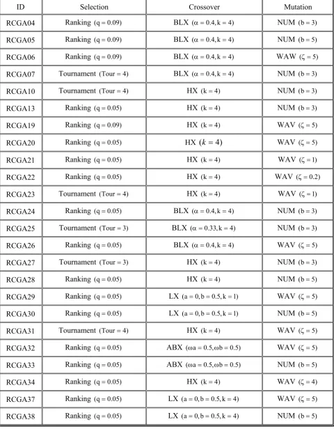
Table 1 show 24 different algorithms that were tested with three problem instances.
The present experiments were carried out using the following parameters: the population size is 60, the crossover and mutation probabilities are 0.8, 0.1 respectively. The number of generations in each run is 100. Each algorithm of Table 1 was run 25 times for each sample data set. The Elitism size was set to 1. g parameter in wavelet mutation was set as 10,000.
4.6. Problem Instances
Parameters values and function forms are determined based on studies in a manufacturing environment. S function assumed to be linear piecewise functions so that the impact of batch size on procurement and assembly costs could be represented properly.TABLE 1. Real-Coded Genetic Algorithms.
ID Selection Crossover Mutation
RCGA04 Ranking (q=0.09) BLX (α=0.4,k=4) NUM (b=3)
RCGA05 Ranking (q=0.09) BLX (α=0.4,k=4) NUM (b=5)
RCGA06 Ranking (q=0.09) BLX (α=0.4,k=4) WAW (ζ=5)
RCGA07 Tournament (Tour=4) BLX (α=0.4,k=4) NUM (b=3)
RCGA10 Tournament (Tour=4) HX (k=4) NUM (b=3)
RCGA13 Ranking (q=0.05) HX (k=4) NUM (b=3)
RCGA19 Ranking (q=0.09) HX (k=4) WAV (ζ=5)
RCGA20 Ranking (q=0.05) HX
(
k
=
4
)
WAV (ζ=5)RCGA21 Ranking (q=0.05) HX (k=4) WAV (ζ=1)
RCGA22 Ranking (q=0.05) HX (k=4) WAV (ζ=0.2)
RCGA23 Tournament (Tour=4) HX (k=4) WAV (ζ=1)
RCGA24 Ranking (q=0.05) BLX (α=0.4,k=4) NUM (b=3)
RCGA25 Tournament (Tour=3) BLX (α=0.33,k=4) NUM (b=3)
RCGA26 Ranking (q=0.05) BLX (α=0.4,k=4) WAV (ζ=5)
RCGA27 Tournament (Tour=3) HX (k=4) NUM (b=3)
RCGA28 Ranking (q=0.05) HX (k=4) NUM (b=5)
RCGA29 Ranking (q=0.05) LX (a=0,b=0.5,k=1) WAV (ζ=5)
RCGA30 Ranking (q=0.05) LX (a=0,b=0.5,k=1) NUM (b=5)
RCGA31 Tournament (Tour=4) HX (k=4) WAV (ζ=5)
RCGA32 Ranking (q=0.05) ABX (ωa=0.5,ωb=0.5) WAV (ζ=5)
RCGA33 Ranking (q=0.05) ABX (ωa=0.5,ωb=0.5) NUM (b=5)
RCGA34 Ranking (q=0.05) HX (k=4) WAV (ζ=4)
RCGA37 Ranking (q=0.05) LX (a=0,b=0.5,k=4) WAV (ζ=5)
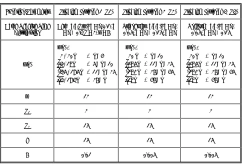
TABLE 2. Problem Instances.
Function/Parameter Problem Instance 1 (P1) Problem Instance 2 (P2) Problem Instance 3 (P3) Batch Receive Time
Distribution
Beta (a,b,p,q): a = d-0.1, b = d + 0.3 p = 2, q = 6
Triangular (a,c,b): a = d-0.05, b = d + 0.15, c = d
Uniform (a,b): a = d-0.05, b = d + 0.15
s(n) ⎪ ⎪ ⎩ ⎪ ⎪ ⎨ ⎧ ≤ + ≤ ≤ + ≤ ≤ + ≤ + = n 26 , n 3 . 18 4 25 n 11 , n 5 . 18 5 . 3 10 n 5 , n 19 3 4 n , n 20 2 ) n ( s ⎪ ⎪ ⎩ ⎪ ⎪ ⎨ ⎧ ≤ ≤ ≤ ≤ ≤ ≤ = n 46 , n 19 45 n 26 , n 2 . 19 25 n 11 , n 5 . 19 10 n , n 20 ) n ( s ⎪ ⎪ ⎩ ⎪ ⎪ ⎨ ⎧ ≤ ≤ ≤ ≤ ≤ ≤ = n 46 , n 19 45 n 26 , n 2 . 19 25 n 11 , n 5 . 19 10 n , n 20 ) n ( s
w 12 12 12
P1 2 2 2
P2 15 15 15
h 15 15 15
λ 0.01 0.005 0.005
solved using different algorithms. As Table 2 shows, three different probability distribution functions (including beta, triangular and uniform) have been used. The Beta distribution can be used to model events which are constrained to take place within an interval defined by a minimum and maximum value. For this reason, the Beta along with the triangular distribution-is used extensively in PERT, CPM and other project management/control systems to describe the duration of an activity. Beta probability density function with parameters p, q distributed over the interval a, b is:
1 q , p , b x a , ) q , p ( aˆ 1 q p ) a b ( 1 q ) x b ( 1 p ) a x ( ) x (
f < < >
− + − − − − − = (17)
In which a, b are lower and upper limits of the beta random variable. Parameters p and q determine the shape of beta distribution. Mean and variance of beta are calculated by:
2 ) q p )( 1 q p ( 2 ) a b ( pq 2 , a q p q b q p p + − + − = σ + + + = μ (18) Figure 1 shows a sample beta pdf in which a, b are
0.3, 0.8 respectively. Mean of this random variable is 0.425. In the data set 1, p, q were considered to be 2, 6 and a, b to be functions of batch due date (d) which means that batch receive time is a beta random variable whose upper and lower limits are
0.3 d b , 0.1 -d
a= = + respectively.
Figure 1. Beta probability density function with parameters 2, 6.
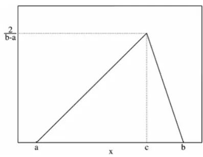
Figure 2. Triangular probability density function.
distribution defined on the range x∈
[ ]
a,b with probability density and distribution functions⎪ ⎪ ⎩ ⎪ ⎪ ⎨ ⎧
≤ < − −
− −
≤ ≤ − −
− =
⎪ ⎪ ⎩ ⎪⎪ ⎨ ⎧
≤ < − −
−
≤ ≤ − −
−
=
b x c ) c b )( a b (
2 ) x b ( 1
c x a ) a c )( a b (
2 ) a x ( )
x ( F
, b x c ) c b )( a b (
) x b ( 2
c x a ) a c )( a b (
) a x ( 2 ) x ( f
(19)
Figure 2 depicts the triangular pdf.
4.7. Model Verification
Model verification is often defined as “ensuring that the computer program of the computerized model and its implementation are correct” and the definition is adopted here. The following techniques are used for model verification:4.7.1. Structured programming and program modularity The computer program has been designed, developed, and implemented using techniques found in software engineering. These include such techniques as structured programming and program modularity. Totally 24 functions and 15 procedures constitute the overall program that could be partitioned in 2 main modules (objective function calculation and genetic algorithm). This modularity makes the program more traceable. 4.7.2. Testing Three testing techniques were used: Structured walk-through: These are step-by-step reviews of program to assure that it behaves correctly.
Unit test: this type of testing is oriented to discovering defects in the individual functions and procedures making up the program. For example, functions written for beta distribution function were tested in this step.
Integration test: These are tests at the module and program level. As higher levels of integration are reached the purpose of testing moves from predominantly verification to validation. These groups should be tested to see if they work together properly as the program is built. For example, objective function is a module that was tested in this way.
TABLE 3. Optimum Solutions.
Problem n a b d Fitness
P1 13 0.0622 0.00145 0.03833 20.05777
P2 26 0.0633 0.00141 0.00136 20.2903
P3 26 0.1006 0.00356 -0.02364 20.4640
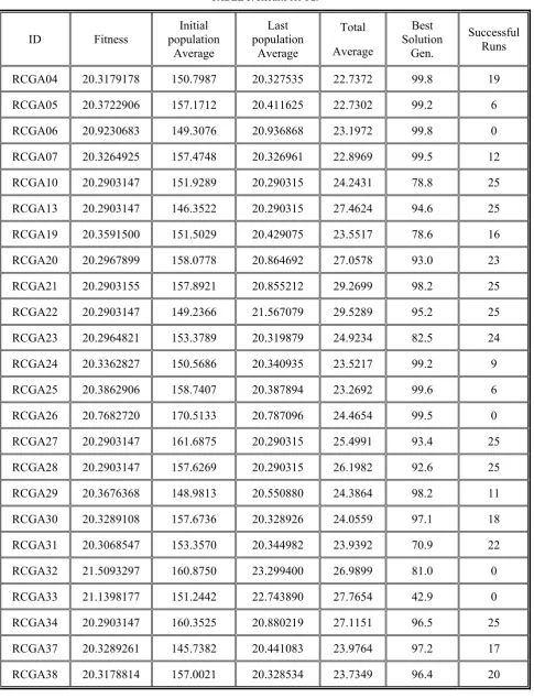
TABLE 4. Problem Instances.
ID Fitness Initial population
Average
Last population
Average
Total Average
Best Solution
Gen.
TABLE 5. Results for P2.
ID Fitness Initial population
Average
Last population
Average
Total Average
Best Solution
Gen.
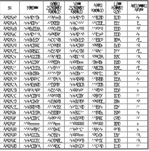
TABLE 6. Results for P3.
ID Fitness Initial population
Average
Last population
Average
Total Average
Best Solution Gen.
Successful Runs
RCGA04 20.5834359 161.36 20.583461 23.2912 99.2 2
RCGA05 20.6045089 158.78 20.604510 22.9444 98.4 1
RCGA06 21.0556529 159.53 21.072663 23.5274 99.2 0
RCGA07 20.5673691 157.14 20.567529 23.2800 99.2 2
RCGA10 20.4743162 148.07 20.474320 24.7782 96.8 23
RCGA13 20.4701713 161.99 20.470195 27.1952 97.5 24
RCGA19 20.5110514 162.69 20.539689 24.0052 92.6 17
RCGA20 20.4743190 156.03 20.572707 27.0499 91.4 23
RCGA21 20.4640564 159.09 20.786432 30.3777 95.9 24
RCGA22 20.4640546 161.33 21.545295 30.5182 90.6 25
RCGA23 20.4654835 166.36 20.495321 25.5842 97.0 24
RCGA24 20.5489485 156.39 20.549045 23.8561 98.6 9
RCGA25 20.5801834 168.79 20.580366 23.5307 99.5 1
RCGA26 21.0731202 153.90 21.099351 24.4922 99.2 0
RCGA27 20.4640497 162.79 20.464056 25.6914 98.2 25
RCGA28 20.4640495 156.29 20.464051 26.4296 97.7 25
RCGA29 20.5255613 152.73 20.657026 24.7777 96.4 13
RCGA30 20.5008146 160.33 20.500947 24.4406 98.2 18
RCGA31 20.5090685 163.63 20.537408 24.6862 94.9 17
RCGA32 21.4778228 155.84 23.997060 27.1444 66.2 0
RCGA33 21.2324508 157.66 23.844241 27.3270 91.2 0
RCGA34 20.4701840 156.48 20.673386 26.9250 91.5 23
RCGA37 20.5767227 161.95 20.624625 24.5855 97.8 5
population is low. Successful runs is the number of runs in which the deviation of the found solution from the optimum fitness is at most 1×10⁻⁵. Hence, a success was counted when the following condition was me
5 10 opt f 1
f − ≤ −
Where fopt is the known global minimum of the problem and f1 is the best value obtained by an algorithm.
Experiment results show that crossover operator is the most important part of the algorithm; because the crossover operator has significant effect on performance of the algorithms. The HX crossover presents the best performance (algorithms RCGA28, RCGA34, RCGA27, RCGA21 and RCGA13) and after it, the LX shows better performance (RCGA30) but the worst results are obtained from BLX and ABX (RCGA32, RCGA33). With normalized geometric ranking, q = 0.05 and with tournament selection, Tour = 3 have a better result.
Total average of the best algorithms is significantly higher than of other algorithms which show that these algorithms are more explorative than others.
5. CONCLUSIONS
In this paper, the problem of due date assignment in make-to-demand production systems were characterized and an original model were presented for it. The main focus was on products with relatively low demand rates. In such cases, the economy of scale??? could not be ignored. On the other hand, quoted lead time and due date related costs must be considered. A model was formulated for such a problem. In the lot sizing literature, the lead time and due date related costs and in the due date assignment literature, economy of scale are ignored. In this paper both were considered. A real-coded genetic algorithm was developed for solving the model.
Assumptions are based on a specific company. The approach used in this paper may be
applied to other production systems. Below are some of the possible extensions:
• Demand may be considered stochastic. • Each customer may order more than one unit
of product. The customer order quantity may follow a probability distribution.
• Long quoted lead times may lead to lost sales.
• Constraints like resource availability may be considered.
6. REFERENCES
1. Dupon, A., Van Nieuwenhuyse, I. and Vandaele, N., “The impact of sequence changes on product lead time”,
Robotics and Computer Integrated Manufacturing,
Vol. 18, (2002), 327-333.
2. Claudio Garavelli, A., “Performance analysis of a batch production system with limited flexibility”, Int. J. Production Economics, Vol. 69, (2001), 39-48.
3. Haskose, A., Kingsman, B. G. and Worthington, D., “Performance analysis of make-to-order manufacturing systems under different workload control regimes”, Int. J. Production Economics, Vol. 90, (2004), 169-186.
4. Dolgui, A. and Ould-Louly, M. A., “A model for supply planning under lead time uncertainty”, Int. J. Production Economics, Vol. 78, (2002), 145-152. 5. Me´ndez, C. A., Henning, G. P. and Cerda, J., “Optimal
scheduling of batch plants satisfying multiple product orders with different due-dates”, Computers and Chemical Engineering, Vol 24, (2000), 2223-2245. 6. Sung, C. S. and Kim, Y. H., “Minimizing due date
related performance measures on two batch processing machines”, European Journal of Operational Research, Vol. 147, (2003), 644-656.
7. Sox, C. R., Jackson, P. L., Bowman, A. and Muckstadt, J. A., “A review of the stochastic lot scheduling problem”, Int J. Production Economics, Vol. 62,
(1999), 181-200.
8. Moon, C., Kim, J. and Hur, S., “Integrated process planning and scheduling with minimizing total tardiness in multi-plants supply chain”, Computers and Industrial Engineering, Vol. 43, (2002), 331-349.
9. Potts, C. N. and Kovalyov, M. Y., ”Scheduling with batching: A review”, European Journal of Operational Research, Vol. 120, (2000), 228-249.
10. Donk, D. P. V., “Make to stock or make to order: The decoupling point in the food processing industries”, Int. J. Production Economics, Vol. 69, (2001), 297-306.
11. Song, D. P., Hicks, C. and Earl, C. F., “Product due date assignment for complex assemblies”, Int. J. Production Economics, Vol. 76, (2002), 243-256.
in multi-machine Job Shops”, Computers and Industrial Engineering, Vol. 41, (2001), 77-94.
13. Veral, E. A. and Mohan, R. P., “A two-phased approach to setting due-dates in single machine job shops”,
Computers and Industrial Engineering, Vol. 36,
(1999), 201-218.
14. Laan, E. V. D., Salomon, M. and Dekker, R., “An investigation of lead-time effects in manufacturing/remanufacturing systems under simple PUSH and PULL control strategies”, European Journal of Operational Research, Vol. 115, (1999),
195-214.
15. Croce, F. D., Gupta, J. N. D. and Tadei, R., “Minimizing tardy jobs in a flowshop with common due date”, European Journal of Operational Research,
Vol. 120, (2000), 375-381.
16. Easton, F. F., Moodie, D. R., “Pricing and lead time decisions for make-to-order firms with contingent orders”, European Journal of Operational Research,
Vol. 116, (1999), 305-318.
17. Reiner, G. and Trcka, M., “Customized supply chain design: Problems and alternatives for a production company in the food industry. A simulation based analysis”, Int. J. Production Economics, Vol. 89,
(2004), 217-229.
18. Habchi, G. and Labrune, Ch., “Study of lot sizes on job shop systems performance using simulation”,
Simulation Theory and practice, Vol. 2, (1995),
277-289.
19. Mosheiov, G., “A common due-date assignment problem on parallel identical machines”, Computers and Operations Research, Vol. 28, (2001), 719-732.
20. Mosheiov, G. and Yovel, U., “Minimizing weighted earliness-tardiness and due-date cost with unit processing-time jobs”, European Journal of Operational Research, Vol. 172, (2006), 528-544.
21. Mosheiova, G. and Oronb, D., Ritovc, Y., “Minimizing flow-time on a single machine with integer batch sizes”,
Operations Research Letters, Vol. 33, (2005), 497-501. 22. Soroush, H. M., “Sequencing and due-date
determination in the stochastic single machine problem with earliness and tardiness costs”, European Journal of Operational Research, Vol. 113, (1999), 450-468.
23. Ooijen, H. P. G. V. and Bertrand, J. W. M., “Economic due-date setting in job-shops based on routing and workload dependent flow time distribution functions”,
Int. J. Production Economics, Vol. 74, (2001),
261-268.
24. Sabuncuoglu, I. and Comlekci, A., “Operation-based flowtime estimation in a dynamic job shop”, Omega,
Vol. 30, (2002), 423-442.
25. Gupta, J.N.D., KruK ger, K., Lauff, V., Werner, F., Sotskov, Y.N., “Heuristics for hybrid flow shops with controllable processing times and assignable due dates”,
Computers and Operations Research, Vol. 29, (2002),
1417-1439.
26. Jahnukainen, J. and Lahti, M., “Efficient purchasing in make-to-order supply chains”, Int. J. Production Economics, Vol. 59, (1999), 103-111.
27. Bertrand, J. W. M. and Sridharan, V., “A study of simple rules for subcontracting in make-to-order
manufacturing”, European Journal of Operational Research, Vol. 128, (2001), 509-531.
28. Bertrand, J. W. M. and Ooijen, H. P. G. V., “Customer order lead times for production based on lead time and tardiness costs”, Int. J. Production Economics, Vol. 64,
(2000), 257-265.
29. So, K. C. and Zheng, X., “Impact of supplier's lead time and forecast demand updating on retailer’s order quantity variability in a two-level supply chain”, Int. J. Production Economics, Vol. 86, (2003), 169-179. 30. Ozdamar, L. and Yazgac, T., “Capacity driven due date
settings in make to order production systems”, Int. J. Production Economics, Vol. 49, (1997), 29-44.
31. Rodrigues, L. A., Graells, M., Cant, J., Gimeno, L., Rodrigues, M. T. M., Espufta, A. and Puigjaner, L., “Utilization of processing time windows to enhance planning and scheduling in short term multipurpose batch plants”, Computers and Chemical Engineering,
Vol. 24, (2000), 353-359.
32. Badell, M. and Puigjaner, L., “Advanced enterprise resource management systems for the batch industry, The TicTacToe algorithm”, Computers and Chemical Engineering, Vol. 25, (2001), 517-538.
33. Hegedus, M. G. and Hopp, W. J., “Due date setting with supply constraints using MRP”, Computers and Industrial Engineering, Vol. 39, (2001), 293-305.
34. ElHafsi, M., “An operational decision model for lead-time and price quotation in congested manufacturing systems”, European Journal of Operational Research,
Vol. 126, (2000), 355-370.
35. Park, M. W. and Kim, Y. D., “A branch and bound algorithm for a production scheduling problem in an assembly system under due date constraints”, European Journal of Operational Research, Vol. 123, (2000),
504-518.
36. Birman, M., Mosheiov, G., “A note on a due-date assignment on a two-machine flow-shop”, in Computers and Operations Research, Vol. 31, (2004),
473-480.
37. He, Q. M., Jewkes, E. M. and Buzacott, J., “Optimal and near-optimal inventory control policies for a make-to-order inventory-production system”, European Journal of Operational Research, Vol. 141, (2002),
113-132.
38. Kolisch, R., “Integration of assembly and fabrication for make-to-order production”, Int. J. Production Economics, Vol. 68, (2000), 287-306.
39. Ray, S. and Jewkes, E. M., “Customer lead time management when both demand and price are lead time sensitive”, European Journal of Operational Research, Vol. 153, (2004), 769-781.
40. Herrera, F., Lozano, M. and Verdegay, J. L., “Tackling real-coded genetic algorithms: operators and tools for the behavioral analysis”, Artificial Intelligence Reviews, Vol. 12, (1998), 265-319.
41. Houck, C. R., Joines, J. A. and Kay, M. G., “A genetic algorithm for function optimization: A Matlab implementation”, NCSUIE Technical Report, (1995), 95-09.
mutation operations”, Soft Comput, Vol. 11, (2007),
7-31.
43. Arumugam, M. S. and Rao, M. V. C., Palaniappan, R., “New hybrid genetic operators for real coded genetic algorithm to compute optimal control of a class of hybrid systems”, Applied Soft Computing, Vol. 6,
(2005), 38-52.
44. Kaelo, P. and Ali, M. M., “Integrated crossover rules in real coded genetic algorithms”, European Journal of Operational Research, Vol. 176, (2007), 60-76. 45. Deep, K. and Thakur, M., “A new crossover operator
for real coded genetic algorithms”, Applied Mathematics and Computation, Vol. 188, (2007),
895-911.
46. Eshelman, L. J. and Schaffer, J. D., “Real coded genetic algorithms and interval schemata”, L. Darrell Whitley, editor, FOGA-2. Morgan Kaufmann, (1993), 187-202. 47. Michalewicz, Z., “Genetic algorithms + Data structures
= Evolution programs”, Springer-Verlag, NewYork, (1992).
48. Joines, J. A. and Houck, C. R., “On the use of
non-stationary penalty functions to solve nonlinear constrained optimization problems with genetic algorithms”, Proceedings of the First IEEE Conference on Evolutionary Computation, (1994),
579-584.
49. Wright, A. H., “Genetic algorithms for real parameter optimization”, G. J. E. Rawlins (Ed.), Foundations of Genetic Algorithms I,Morgan Kaufmann, San Mateo,
(1991), 205-218.
50. Meittinen, K., Makela, M. M. and Toivanen, J., “Numerical comparision of some penalty based constraint handling techniques in genetic algorithms”, Journal of Global Optimization, Vol. 27, (2003), 427-446.
51. Herrera, F., E. Herrera-Viedma, Lozano, M. and Verdegay, J. L., “Fuzzy tools to improve genetic algorithms”, Proc. second European Congress on Intelligent Techniques and Soft Computing, (1994),
1532-1539.