A Bi-objective Stochastic Optimization Model for Humanitarian Relief Chain by Using Evolutionary Algorithms

(1)

Please cite this article as: N. Javadian, S. Modarres, A. Bozorgi, A Bi-objective Stochastic Optimization Model for Humanitarian Relief Chain by Using Evolutionary Algorithms, International Journal of Engineering (IJE), TRANSACTIONS A: Basics Vol. 30, No. 10, (October 2017) 1526-1537

International Journal of Engineering

J o u r n a l H o m e p a g e : w w w . i j e . i r

A Bi-objective Stochastic Optimization Model for Humanitarian Relief Chain by

Using Evolutionary Algorithms

N. Javadian*a_{, S. Modarres}a_{, A. Bozorgi}b

a_{Mazandaran University of Science and Technology, Mazandaran, Iran}

b_{School of Industrial Engineering, College of Engineering, University of Tehran, Tehran, Iran}

P A P E R I N F O

Paper history:

Received 07 March 2017

Received in revised form 21 June 2017 Accepted 07 July 2017

Keywords: Lines of Code Uncertainty ɛ-constraint Method Emergency Logistics Humanitarian Relief Chain Evolutionary Algorithms

A B S T R A C T

Due to the increasing amount of natural disasters such as earthquakes and floods and unnatural disasters such as war and terrorist attacks, Humanitarian Relief Chain (HRC) is taken into consideration of most countries. Besides, this paper aims to contribute humanitarian relief chains under uncertainty. In this paper, we address a humanitarian logistics network design problem including local distribution centers (LDCs) and multiple central warehouses (CWs) and develop a scenario-based stochastic programming (SBSP) approach. Also, the uncertainty associated with demand and supply information as well as the availability of the transportation network's routes level after an earthquake are considered by employing stochastic optimization. While the proposed model attempts to minimize the total costs of the relief chain, it implicitly minimize the maximum travel time between each pair of facility and the demand point of the items. Additionally, a data set derived from a real disaster case study in the Iran area, and to solve the proposed model a exact method called ɛ-constraint in low dimension along with some well-known evolutionary algorithms are applied. Also, to achieve good performance, the parameters of these algorithms are tuned by using Taguchi method. In addition, the proposed algorithms are compared via four multi-objective metrics and statistically method. Based on the results, it was shown that: NSGA-II shows better performances in terms of SNS and CPU time, meanwhile, for NPS and MID, MRGA has better performances. Finally, some comments for future researches are suggested.

doi: 10.5829/ije.2017.30.10a.14

1. INTRODUCTION1

In recent years, many areas around the world have been affected by natural disasters

.

These events are leading to the death, injury and destruction of property and disruption of daily activities that these unpleasant experiences are considered as natural disasters [1]. Moreover, disasters can be natural (such as earthquake, famine, tsunami, cyclone, hurricane, flood, etc.), manmade disasters (such as terrorism, war, civil disorder, etc.), disease (like HIV/aids or malaria) or extreme poverty situation.

The rate of natural disasters is increasing intensely due to population growth, global inclination in

*Corresponding Author’s Email: [email protected] (N. Javadian)

(2)

beneficiaries. Besides, the high scale of these crises, has increased the need for efficient management of the relief supply chain

.

Iran is one of the most disaster-prone country in the

world due to its geographical conditions, that destructive earthquakes and the crisis which occurred after its occurrence, every year causing irreparable damage to people and the economy of the country. Existence of an integrated chain of all components and Humanitarian Relief, will be facilitate the disaster management in natural disasters, especially earthquakes that offered to the people involved in the events [2].

Humanitarian Relief Logistics is one of the most important elements of the relief operation in crisis management.Logistics planning in disaster relief are included sending of several items (such as medicine, rescue equipment, rescue teams, food, etc.) from a number of source of supply to multiple points of distribution in damaged areas through a chain structure. Also, the transfer of goods should be done quickly and efficiently so that the survival rate of affected people, and the cost of operations are maximized and minimized, respectively [3].

There are some review articles showing the state of the art in area of HRCs from various viewpoints consisting a general review on HRCs to identify suitable measures in various phases or steps of disasters which are pre-disaster, during-disaster and post-disaster [1, 4-6]. For instance, Caunhye et al. [6] reviewed proposed models for post and pre-disaster operations. In addition, they mentioned proposed models for traffic control and

lifeline rehabilitation. More recently, Özdamar and Ertem [7] presented a survey that focused on the response and recovery planning steps of the disaster lifecycle.

Recently, a three-level relief chain model include suppliers, distribution centers, and affected areas is proposed by Zokaee et al. [2]. They proposed a MILP deterministic model by using stochastic optimization and they considered uncertainty for demand, supply, and all of the cost parameters, where the uncertain parameters are independent and bounded random variables. Their offered model attempts to minimize the total costs of the relief chain, it implicitly maximizes people’s satisfaction level in the affected areas through applying a penalty to shortages of relief commodities. Moreover, a real disaster case study in the Iran for earthquakes is applied to test the efficiency of the suggested model. In addition, Sahebjamnia et al. [8] proposed a Hybrid Decision Support System (HDSS) include a simulator, a rule-based inference engine, and a knowledge-based system in order to design a three level HRC. Three main performance measures including the coverage, total cost, and response time are considered to make an explicit trade-off analysis between cost efficiency and responsiveness of the designed HRC. Also, a real case study in Tehran demonstrate use of

stochastic data. Moreover, some researches paid

attention to earthquake; for example, Yazdani and

Kowsari, Nateghi et al., Rajabipour and Behnamfar and

Yazdani et al. [9-12]. Finally, a brief review of papers in

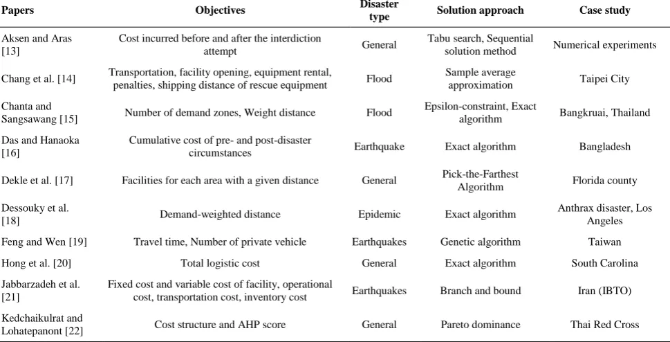
this research area is presented in Table 1.

TABLE 1. A brief review of related works

Papers Objectives Disaster

type Solution approach Case study

Aksen and Aras [13]

Cost incurred before and after the interdiction

attempt General

Tabu search, Sequential

solution method Numerical experiments Chang et al. [14] Transportation, facility opening, equipment rental,

penalties, shipping distance of rescue equipment Flood

Sample average

approximation Taipei City Chanta and

Sangsawang [15] Number of demand zones, Weight distance Flood

Epsilon-constraint, Exact

algorithm Bangkruai, Thailand Das and Hanaoka

[16]

Cumulative cost of pre- and post-disaster

circumstances Earthquake Exact algorithm Bangladesh Dekle et al. [17] Facilities for each area with a given distance General Pick-the-Farthest

Algorithm Florida county Dessouky et al.

[18] Demand-weighted distance Epidemic Exact algorithm

Anthrax disaster, Los Angeles Feng and Wen [19] Travel time, Number of private vehicle Earthquakes Genetic algorithm Taiwan Hong et al. [20] Total logistic cost General Exact algorithm South Carolina Jabbarzadeh et al.

[21]

Fixed cost and variable cost of facility, operational

cost, transportation cost, inventory cost Earthquakes Branch and bound Iran (IBTO) Kedchaikulrat and

(3)

As is clear, some of these researches paid to disaster issues and tried to minimize total costs via exact method. Also, some of them used heuristic and metaheuristic approaches and report the efficiency of these algorithms in their workes.

As one of this paper contribution, we consider two objective function include minimizing costs and minimizing maximum travel time which to the best of

our knowledge simultaneouscompination of them is not reported yet. Moreover, we developed two well-known meta-heuristics along with ɛ-constraint method to solve proposed framework which is another contribution of this paper. Additionally, a data set derived from a real disaster case study in the Iran area.

The structure of this paper is planned as follows: Section 2 and Section 3 presents the problem definition and model formulation, respectively. Section 4 presents Solution approach. In Section 5, parameter tuning process is performed. In Section 6, a computational results is presented. Finally, future research and conclusion are given in Section 7.

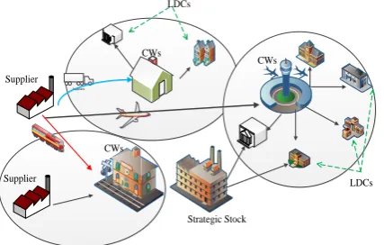
2. PROBLEM DESCRIPTION

The proposed network of disaster relief logistics is presented in Figure 1. The stages are the set of suppliers, the contain CWs and strategic stocks, and the last stage include of local distribution centers (LDCs) in the areas, which are affected by disaster. Hence, suppliers could play as a critical role in the relief chain

and they prepare the required commodities to people in

devastated areas. Those people could play a main role of the customers in the physical distribution. CWs contain warehouses, airports, train station and bus stations. The location of LDCs can be determined on the facilities of fortified existing public as health centers, schools, and mosques which are distributed in all over the city. Using of LDCs is completely justifiable since according to the response agency representatives it is not practical to found a large number of CWs that remain inactive until a disaster strikes.

Suppliers

Strategic Stock Supplier

LDCs CWs

Supplier

LDCs

CWs

Figure 1. Overall structure of HRC

3. MODEL FORMULATION

In this section, the model elements including indices, parameters, and variables are introduced as follows.

Indices

l Index of potential suppliers

i Index of potential CWs j Index of potential LDCs

k Index of affected areas; demand points

h Index of potential strategic stocks

m Index of potential transportation mode

s Index of potential disaster scenarios

q Index of relief items

c Index for storage capacity levels of CWs

g Index of potential sub-sequent disasters

Parameters c

i

F Establishing cost of ith CW at capacity level c

j

G Establishing cost of jth LDC

h

E Establishing cost of hth strategic stocks

q

IH Inventory holding cost of item q

is q

UC Unit inventory cost of unused item q at each CWs i

in disaster scenario s

js q

UL Unit inventory cost of unused item q at each LDCs j

in disaster scenario s

i qs

 Usable inventory ratio of the qth item at the ith CW under scenario s

j qs



Usable inventory ratio of the qth item at the jth LDC under scenario s

s l



Usable capacity ratio of the lth supplier under scenario s

s q

US Unit shortage cost of item q in disaster scenario s

s ijm

TA

Transportation time between the ith CW and jth LDC via mode m to reflect the road and traffic conditions in disaster scenario s

s lim

TB

Transportation time between the lth supplier and the

ith CW via mode m to reflect the road and traffic conditions in disaster scenario s

s ijm



1, if mode m is available under scenario s between the ith CW and jth LDC; 0 otherwise

s lim



1, if mode m is available under scenario s between the lth supplier and ith CW; 0 otherwise

s qk

D Demand level for the qth item at the kth demand

point under scenario s

c

V Storage capacity of each CW established at capacity _level_c

j

(4)

q h

SA Storage capacity of the hth strategic stock for qth

item

ql

CS Storage capacity of the lth supplier for the qth item

ijm

CAP Capacity of transportation mode between ith CW

and jth LDC via mode m

lim

ccp Capacity of transportation mode between the lth

supplier and the ith CW via mode m

qlim

CT Cost of transportation mode between the lth supplier

and the ith CW via mode m for qth item

qijkm

CTR Cost of transportation mode between ith CW and jth

LDC to demand point k via mode m for qth item

q

A Required unit storage capacity of the qth item

s

P Probability of occurring the scenario s

g s



Sub-sequent disasters effects on demands after the major disaster in scenario s (g is the number of minor disaster in scenario s)

g s

 Sub-sequent disasters effects on delivery time after major disaster scenario s (g is the number of minor disaster in scenario s)

ql

 1, if supplier lth capable to deliver qth item

Decision variables

c i

Y 1, if the ith candidate CW is opened at capacity level

c; 0, otherwise

j

O 1, if the jth candidate LDC is opened; 0, otherwise

h

 1, if the hth candidate strategic stock is opened; 0, otherwise

l



1, if the lth candidate supplier is selected; 0, otherwise

qi

R Inventory level of the qth item at the ith CW

qj

U Inventory level of the qth item at the jth LDC

s qi

UI Unused inventory level of the qth item at the ith CW

under disaster scenario s

s qj

UR Unused inventory level of critical item q at the jth

LDC under disaster scenario s

s ijm

N 1, if transportation mode m is selected between ith

CW and jth LDC under scenario s

s lim

C 1, if transportation mode m is selected between lth

supplier and ith CW under scenario s

s qjk

x

Amount of the qth critical item to be delivered from the jth LDC to demand point k under disaster scenario s

s qijkm

z

Amount of the qth item to be delivered from CW i to demand point k via jth LDC and transportation mode m under disaster scenario s

s qhjk

v

Amount of the qth item to be delivered from strategic stock h to demand point k via jth LDC under disaster scenario s

s qlim

w

Amount of the qth item to be delivered from supplier l to the ith CW via transportation mode m under

disaster scenario s

s qk

 Amount of unfulfilled demand for the qth item in demand point k under disaster scenario s

max

T Maximum travel time between each pair of facility _{and the demand point of the items}

Assumptions

The main characteristics and assumptions used in the formulation of resilience HRC model are as follows:

The capability of suppliers and candidate CWs may be partially disrupted by a disaster through damage to the roads and/or destruction to the facility. (Vulnerability of facilities is taken into account through incorporating different usable inventory ratio of each item at each CW/LDS under each scenario to capture supply uncertainty as a result of possible destruction of storage sites (completely or partially) during the disaster;

Each CW is supplied by suppliers (with limited capacity).

Each LDC is supplied by either CWs or multiple CWs or strategic stocks.

Strategic stock is located in the safe places commonly outside of the expected disaster regions.

Each strategic stock ships the items directly not to all the LDCs but nearest ones. (It means, there is the limitation of distance and each strategic stock can ship the items to the LDCs which are located at the acceptable distance far away from strategic stock.

Transportation between suppliers and CWs or strategic stock and LDCs are considered to be multi-mode (Train, Plane, Helicopter, Truck, Motorcycle etc). The capability of each mode or rout may be partially disrupted by a disaster through damage to the roads. In fact, the possible destruction of transportation routes at different levels is considered.

The resiliency level is calculated for each facility (i.e., suppliers, CWs, LDCs).

The multiple disasters or sub-sequent minor disasters are considered for modeling. This study assumes that these minor disasters can affect the time of delivery and increasing the initial demand.

More than one kind of relief commodity must be delivered, and each product is concerned with a various volume and a various cost of procurement, storage, and transportation.

Each supplier and LDC can deliver a given number of relief commodities and it is based on suppliers’ flexibility level.

Inventory may be stored at CWs, LDCs and strategic stocks. Similar to suppliers, each CW, LDC and strategic stock can keep one or several kinds of relief commodity; consequently, they can deliver a given number of service and commodity.

(5)

factors including the disaster scenario and the impact of the disaster.

Several capacity levels are considered for each candidate CW where appropriate capacity should be determined for each selected CW.

Here, we aim to present a bi-objective mixed integer linear programming to specify the location of CWs and LDCs, simultaneously and the corresponding inventory quantities for relief items, and the distribution quantities from supplier to CWs, from CWs to the affected areas (LDC) and from strategic stock to LDC.

. . . .

. . .

.

. .

.

c c

i i j j h h q ki

i c j h q k i

is s js s s s

q qi q qj q qk

q i q j q k

s s s

s qlim qlim qijkm qijkm

q l i m q i j k m

q kj

q k j

Min TC F Y G O E IH R

UC UI UL UR US

P

CT w CTR z

IH U





   

   

 

  

 

 

 



















(1)

max

MinT (2)

Subject to:

. c. c

q qi i

q c

A R  V Y  i I



(3)

1

c i c

Y   i I



(4)

. .

q qj j j q

A U CA O  j J



(5)

(1 )

, ,

s s s s g s

qjk qijkm qhjk qk s qk

j i j m h j g

x z v D

k K q Q s S

 

    

   









(6)

. , ,

s s j qjk qj qs qj k

x UR  U  j J qQ sS



(7)

. , ,

s s i

qijkm qi qs qi

j k m

z UI  R  i I qQ sS



(8)

. . , , ,

s s s

qijkm ijm ijm ijm

q k

z  CAP N  i I jJ mM sS



(9)

. . . , ,

s s qlim ql l ql l i m

w   CS   q Q lL sS



(10)

. . , , ,

s s s

qlim lim lim lim

q

w  CCP C  l L iI mM sS



(11)

. , ,

s q qhjk h h k j

v SA



 h H qQ sS



(12)

. (1 ) . .

, , , ,

s g s s Max

ijm s ijm ijm

g

T A N T

i I j J m M g G s S

 

 

 

 

 

     



₍₁₃₎

max

. (1 ) . .

, , , ,

s g s s

lim s lim lim

g

TB C T

l L i I m M g G s S

 

 

 

 

 

     



₍₁₄₎

. . , , , ,

s s s

qlim lim lim

w M C   l L iI mM qQ sS (15)

. . , , , , ,

s s s

qijkm ijm ijm

z M N   k K jJ iI mM q Q s S (16)

max

, , , , , , , , , 0

, , , , , ,

s s s s s s s qijkm qjk qk qlim qhjk qj qj qi qi

z x w T v UR U R UI

i I j J l L k K h H q Q s S

 

        (17)

 

, , , , , 0,1

, , , , , ,

c s s j i l h ijm lim

O Y N C

i I l L m M c C j J h H s S

  

        (18)

Objective function (1) minimizes the total operating costs of selected CWs and LDCs, and their inventory costs. The last part of objective function (1), minimize total cost of unused inventories and shortage cost of unmet demands and transportation cost of items. Objective function (2) minimizes the maximum travel time between each pair of CW/LDC and demand point for the items.

Constraint (3) enforce restrictions on the available capacity of CWs. Constraint (4) implies that maximum number of CW with specified capacity level which could be constructed at each candidate site is one. Constraint (5) enforces restrictions on the available capacity of LDCs. Constraint (6) determines the unsatisfied demands for critical items. The right hand of

Equation (6) determines initial demand plus demands added after sub-sequent minor disasters. Constraints (7) and (8) ensure that the distributed quantity of each item plus regarded unused inventory is equal to their corresponding inventory levels in respective CW/LDCs. Constraint (9) enforce restrictions on the available capacity of transportation system between pair of CW/LDCs. Constraint (10) enforces restrictions on the available capacity of suppliers. Each supplier can deliver a given number or set of critical items which is depend on suppliers’ flexibility level. Also, each supplier may loss its capacity partially or totally and right hand of constraint (10) guarantees these conditions. Constraint (11) ensures restrictions on the available capacity of transportation system between pair of supplier/CWs. Constraint (12) enforce restrictions on the available capacity strategic stock. Constraints (13) and (14) calculate the maximum travel time. Constraints

(6)

4. SOLUTION APPROACH

In low dimension problem, a exact method called ɛ-constraint is used and due to NP-hardness of the proposed model, exact methods are not proper for large-size problem. Besides, non-dominated sorting genetic algorithm (NSGA-II), non-dominated ranking genetic algorithm (NRGA) are applied to discover Pareto solutions. The mentioned algorithms are used in the same way in recent literature. Moreover, encoding and decoding procedures are illuminated in the following section.

4. 1. Encoding and Decoding Diverse methods have been established to encode the solutions in different models, such as: Michalewicz matrix, Prufer numbers, and priority-based technique.In this paper, the priority-based method is applied. To present the offered array or chromosome,

a

small-size example is shown in this sector to show the procedure of satisfying all the constraints by the suggested form. In this example,

amountsof indices as i=3, l=3, h=2, j=3,c=3,q=2, and

k=2 are assumed. The offered chromosome is a matrix with two rows for each items and (l+2i+h+2j+k) columns which have three sectors. These sectors are considered according to the flows shown in Figure 1. The plan of suggested chromosome is shown in Figure 2.

The matrix shown in Figure 2 is randomly generated and all elements of first row of this matrix are set to random numbers in the interval [0, 1], and all elements of second row of this matrix are filled by uniform~ [1, c]. After sorting the values of first row and rounding the values of second row, the priority-based matrix is achieved. In addition, sorting of each segment, for each sub-segment, is done separately. The plan of suggested priority-based chromosome is shown in Figure 3.

Segment one presents the amount of shipped goods from suppliers (l) to CWs (i). Segment two presents the amount of shipped goods from CWs and strategic stocks (h+i) to LDCs (j). Also, segment three presents the amount of shipped goods from LDCs (j) to affected areas (k).

Segment 1 Segment 2 Segment 3

It em n o d e

l i h+i j j k

1 Pr. 0 .0 7 2 0 .1 3 2 0 .7 8 6 0 .9 5 8 0 .7 9 9 0 .6 4 1 0 .3 8 5 0 .6 5 0 0 .8 9 7 0 .6 7 4 0 .1 1 5 0 .2 4 3 0 .1 2 2 0 .4 9 0 0 .9 8 6 0 .2 1 8 0 .5 1 6 0 .0 2 6 0 .3 4 6 C .L. 1 .5 2 6 1 .2 6 8 1 .2 0 9 1 .5 6 2 2 .1 2 3 2 .5 4 4 2 .7 3 8 1 .7 2 6 2 .7 8 3 1 .8 6 0 1 .1 6 8 1 .4 6 9 2 .9 8 9 1 .7 1 6 2 .2 8 9 1 .2 3 9 2 .4 5 7 2 .7 2 3 1 .1 9 9 2 Pr. ₀.09

9 0 .3 3 2 0 .0 3 4 0 .3 8 3 0 .3 3 9 0 .4 3 1 0 .9 9 7 0 .3 5 0 0 .7 9 2 0 .3 1 3 0 .8 5 2 0 .5 1 2 0 .3 9 1 0 .3 8 2 0 .4 7 2 0 .3 0 4 0 .8 9 4 0 .4 7 1 0 .6 3 5 C .L. 2 .7 3 8 1 .7 2 6 2 .7 8 3 1 .8 6 0 1 .1 6 8 1 .4 6 9 2 .9 8 9 1 .7 1 6 2 .2 8 9 1 .2 3 9 2 .4 5 7 2 .7 2 3 1 .1 9 9 1 .5 2 6 1 .2 6 8 1 .2 0 9 1 .5 6 2 2 .1 2 3 2 .5 4 4

Figure 2. Plan of random key chromosome

Segment 1 Segment 2 Segment 3

It em n o d e

l i h+i j j k

1

Pr. 1 2 3 3 2 1 2 3 5 4 1 2 1 3 3 1 2 1 2

C

.L. * * * 2 2 3 * * 3 2 1 * * * * * * * *

2

Pr. 3 2 1 2 1 3 5 2 3 1 4 3 2 1 2 1 3 1 2

C

.L. * * * 2 1 1 * * 2 1 2 * * * * * * * *

Figure 3. Plan of priority-based chromosome

Moreover, Capacity level of each CWs (i) is presented in second row of proposed chromosome. Furthermore, allocation procedure is presented in Figure 4 which for each segment can be used from needed steps of it.

Figure 4. The allocation procedure

4. 2. NRGA and NSGA-II Usually, the real world issues and decisions are often complex, hence they cannot be solved by the exact methods in a proper time and cost [23, 24]. NSGA-II, offered by Deb et al. and NRGA, proposed by Al Jaddan et al., as two strong well-known multi-objective algorithms are utilized to evaluate the performance of solutions [25, 26]. The

For s=1:S For q=1:Q

Inputs: I: set of source J: set of applicant

Djs: demand of applicant j under scenario s

Cais: capacity of source i under scenario s

V(I+J): Encode solution of item q for scenario s

Outputs:

Xalocijs: amount of shipment between nodes under scenario s

Yj: binary variable shows the opened applicant

Uqis: amount of unused item q of source i under scenario s

Uqjs: amount of unused item q of applicant j under scenario s

0 & & 0

is js

i j

W hileCa   D 

Step1: Xalocijs0  i I j, J

Step2: select value of first column of sub-segment I for i index

select value of first column of sub-segment J for j index

Step3: Xalocijs=min(Cais , Djs)

Update demands and capacities

Cais= Cais - Xalocijs Djs= Djs - Xalocijs

Step4: if Cais=0 then V(1,I)=0

if Djs =0 then V(1,J)=0

End while

Step5: Uqis=Cais Uqjs =Djs

End for

Step6: for j= 1 to J

if ₀

ijs s jX aloc 

 

then Yj=1

(7)

chromosome structure and the function evaluation procedure in NSGA-II and NRGA algorithms are similar to each. The only difference between these algorithms is in their selection mechanism. NSGA-II uses binary tournament selection strategy while NRGA uses Roulette wheel selection strategy. Moreover, four types of mutation operators including reversion mutation, insertion mutation, continuous mutation, and swap mutation are used in local search sector of these algorithm. Furthermore, three types of crossover operators including single-point crossover, double-point crossover, and uniform crossover are utilized in these algorithms to enhance their performances. The main structure of these two algorithms is provided in literatures [25, 26].

4. 3. Performance Metrics Four performance are used in this sector to evaluate the performance of the above-mentioned multi-objective evolutionary algorithms.

Number of Pareto solution (NPS): The number of Pareto optimal solutions is offered by this metric. The more number of Pareto solutions in an algorithm is better performance.

Mean ideal distance (MID): This metric is used to compute the distances between the Pareto fronts and the ideal point. The value of this metric is calculated by Equation (19) :

2 2

1

1 1 2 2

n _i _best _i _best max min max min i

total total total total

f f f f

MID

n 

   _  

 _   _ 

   





(19)

In this equation, n is the number of non-dominated solutions, and f1i and f2i are the value of i

th

non-dominated solution for each objective functions, respectively. (f1best, f2best) is the ideal point which

characterizes the point (0,0) in this problem. fjtotalmax,

fjtotal min

are the smallest and the biggest values of every fitness function among all non-dominated solutions resulted from an algorithm, respectively.

The less the value of MID, the better algorithm’s performance.

 Spread of non-dominance solution (SNS): To assess the diversity of Pareto solutions, this metric is applied and is framed as Equation (20):





2

1

n

i

i MID C

SNS

n

 







₍₂₀₎

Where,

2 2

1 2

i i i

C  f f

 Computational time (CPU time): The speed of running the algorithms to find near optimum solutions is one of the most important indices to evaluate the performance of an algorithm.

5. PARAMETERS SETTING

Here, the parameter tuning process is performed both on the parameters of the algorithms and on the model parameters in the following two subsections, respectively.

5. 1. Parameter Tuning

Here, in order to tuning the values of the algorithms' parameters, the Taguchi method is applied [27]. This effective method proposed by Taguchi and this method is utilized instead of the full factorial experimental design. Multi-objective algorithms are assessed according to multi-objective measures. Also, Equation (21) presents the selected response of Taguchi method in this study. The advantage of this response is that it considers both of the two main features of multi-objective algorithms entitled diversity and convergence.

MID MCOV

SNS

 (21)

The first step to produce a Taguchi design is identify the levels of each factors of algorithms. This step is shown in Table 2 where each factor has three levels. Then, by using Minitab ® software and applying the Taguchi method the L9

orthogonal array

for NRGA, NSGA-II

algorithms are designated. The orthogonal arrays of each algorithm along with the achieved results are displayed in Table 3.

For each algorithm, the related S/N ratio chart obtained by the Minitab® software is shown in Figure 5-6. In this figure, the best level of each factor is selected to be the one with the highest S/N ratio. Besides, {Pc=0.7, Pm=0.1, N-pop=100, Max-iteration =100} are the selected parameters for NSGA-II and {Pc=0.7, Pm=0.15, N-pop=50, Max-iteration =200} are the selected parameters for NRGA by using the Figures 5 and 6.

Moreover, it should be notice that the Taguchi experiment is perform for the first test problem of Table 4 and for other test problems these tuned parameters are utilized.

TABLE 2. Algorithm parameter ranges along with their levels

Algorithms parameters Parameter level Level 1 Level 2 Level 3

NSGA-II

Pc 0.7 0.8 0.9

Pm 0.05 0.1 0.15

N-pop 50 100 150

Max-iteration 100 200 300

NRGA

Pc 0.7 0.8 0.9

Pm 0.05 0.1 0.15

N-pop 50 100 150

(8)

TABLE 3. The orthogonal array L9 and results for the algorithms

Run Pc Pm Npop Max-iter NRGA NSGA-II

1 1 1 1 1 1.5426e-011 1.7548e-011 2 1 2 2 2 2.3523e-011 2.3432e-011 3 1 3 3 3 1.8792e-011 2.7898e-011 4 2 1 2 3 3.4582e-011 3.1347e-011 5 2 2 3 1 3.1835e-011 1.7458e-011 6 2 3 1 2 1.7481e-011 5.5568e-011 7 3 1 3 2 2.5756e-011 4.2356e-011 8 3 2 1 3 2.9625e-011 2.8796e-011 9 3 3 2 1 2.7452e-011 1.5143e-011

Figure 5. Signal to noise plot of NSGA-II

Figure 6. Signal to noise plot of NRGA

Also, in performing of Taguchi experiment, the "smallest response is better" as a selected response for identifying of parameters is used.

5. 2. Case Study In this section, to accumulation of the proposed model's parameters, a case study in Iran is applied. In this respect, the proposed model is applied on the case study to demonstrate the correctness and appropriateness of the results. In fact, this research is stimulated regarding to the complex issue of designing a HRC in Mazandaran province in Iran. Accordingly, we provide details of the case study for the design of HRC

in one of the northern province of Iran, Mazandaran; aiming at better response to a potential disasters. The province covers a region of 23,842 km². In addition, Mazandaran is one of the most thickly populated provinces in Iran and has various natural resources, especially large reservoirs of oil and natural gas. The population of the province was 2,922,432 regarding to the census of 2006, in which 46.82% villagers, 53.18% were urban dwellers, and remaining were non-residents.

Increasing the number of disruption scenarios represented that the leads to computational time could be increased. Meanwhile, the number of scenarios which is considered for the network design problems is 3 disruption scenarios in our case study.

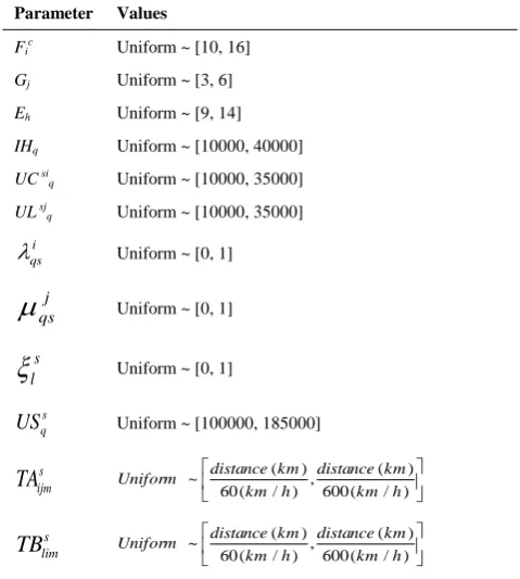
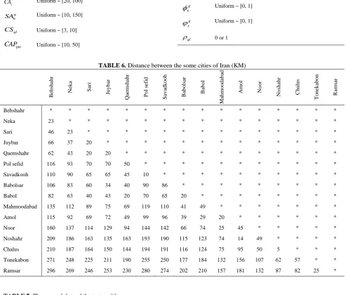
The level of a disaster scenario depends on the occurrence time which are separately presented in the Table 4. The proposed mathematical model is coded in the MATLABTM 2010 software and regarding to a Pentium dual-core 2.5 GHz computer with 4 GB RAM is solved. Moreovere, other parameters of proposed model such as: the general data of the test problems and other parameters are presented in Tables 5-7.

TABLE 4. Probabilities of different earthquake scenarios Disaster scenarios Probability Number

Scenario 1 0.453 3

Scenario 2 0.345 2

Scenario 3 0.202 1

TABLE 5. Other model parameters tuning Parameter Values

Fic Uniform ~ [10, 16]

Gj Uniform ~ [3, 6]

Eh Uniform ~ [9, 14]

IHq Uniform ~ [10000, 40000]

UC si

q Uniform ~ [10000, 35000] UL sjq Uniform ~ [10000, 35000]

i qs



Uniform ~ [0, 1]

j qs



Uniform ~ [0, 1]

s l



Uniform ~ [0, 1]

s q

US Uniform ~ [100000, 185000]

s ijm

TA

~ ( ), ( )

60 ( / ) 600 ( / )

distance km distance km Uniform

km h km h

 

 

 

s lim

TB

~ ( ), ( )

60 ( / ) 600 ( / )

distance km distance km Uniform

km h km h

 

 

 

3 2 1 216

214

212

210

208

3 2 1

3 2 1 216

214

212

210

208

3 2 1 Pc

M

ea

n

of

S

N

ra

tio

s

Pm

N-pop Maxiter

Data Means

Signal-to-noise: Smaller is better

3 2 1 214

213

212

211

3 2 1

3 2 1 214

213

212

211

3 2 1 Pc

M

ea

n

of

S

N

ra

tio

s

Pm

N-pop Maxiter

Data Means

(9)

s ijm



0 or 1

s lim



0 or 1

s qk

D Uniform ~ [50, 300]

V c _{Uniform ~ [80, 250]} j

CA Uniform ~ [20, 100]

q h

SA Uniform ~ [10, 150]

ql

CS Uniform ~ [3, 10]

ijm

CAP Uniform ~ [10, 50]

lim

CCP Uniform ~ [4, 10]

qlim

CT Uniform ~



distance km( ) 10000( ), R distance km( ) 100000( ) R



qijkm

CTR Uniform ~



distance km( ) 10000( ), R distance km( ) 100000( ) R



Aq Uniform ~ [0.01, 0.4]

Ps [0.2, 0.5, 0.3]

g s

 Uniform ~ [0, 1]

g s

 Uniform ~ [0, 1]

ql

 0 or 1

TABLE 6. Distance between the some cities of Iran (KM)

B

eh

sh

ah

r

N

ek

a

S

ar

i

Ju

y

b

ar

Q

ae

ms

h

ah

r

P

o

l

se

fi

d

S

av

ad

k

o

h

B

ab

o

lsar

B

ab

o

l

M

ah

m

o

d

ab

ad

A

mo

l

N

o

r

N

o

sh

ah

r

C

h

al

u

s

To

n

ek

ab

o

n

R

ams

ar

Behshahr * * * * * * * * * * * * * * * *

Neka 23 * * * * * * * * * * * * * * *

Sari 46 23 * * * * * * * * * * * * * *

Juybar 66 37 20 * * * * * * * * * * * * *

Qaemshahr 62 43 20 20 * * * * * * * * * * * *

Pol sefid 116 93 70 70 50 * * * * * * * * * * *

Savadkooh 110 90 65 65 45 10 * * * * * * * * * *

Babolsar 106 83 60 34 40 90 86 * * * * * * * * *

Babol 82 63 40 43 20 70 65 20 * * * * * * * *

Mahmoodabad 135 112 89 75 69 119 110 41 49 * * * * * * *

Amol 115 92 69 72 49 99 96 39 29 20 * * * * * *

Noor 160 137 114 129 94 144 142 66 74 25 45 * * * * *

Noshahr 209 186 163 135 163 193 190 115 123 74 14 49 * * * * Chalus 210 187 164 150 144 194 191 116 124 75 95 50 5 * * * Tonekabon 271 248 225 211 190 255 250 177 184 132 156 107 62 57 * * Ramsar 296 269 246 253 230 280 274 202 210 157 181 132 87 82 25 *

TABLE 7. The general data of the test problems

Test L I J K H M S Q C G

1 3 2 3 2 2 2 3 4 2 1

2 5 3 5 3 2 3 3 6 3 2

3 7 4 7 5 3 3 3 9 3 3

4 9 6 9 6 5 3 3 10 5 5 5 11 7 11 8 6 3 3 15 6 5 6 12 9 14 10 7 3 3 18 8 6 7 13 10 16 13 9 3 3 20 10 7

8 16 12 19 14 10 3 3 22 12 8 9 17 15 21 18 11 3 3 25 15 9 10 18 18 23 20 13 3 3 30 20 10

6. COMPUTATIONAL RESULTS

(10)

the algorithms on the 10 test problems introduced in Section 5.2. To validate proposed approaches, ɛ-constraint method is used in low dimension problems. As is clear, two developed metaheuristics have a near behavior with ɛ-constraint method which it refers to efficiency of them.

In order to compare the obtained metrics, analysis of variance (ANOVA) is used. The results prove that there is a clear statistically significant difference between performances of the algorithms. The intervals plot (at the 95% confidence level) for these algorithms for each metric are shown in Figures 7-10. Each interval plot has three points for each algorithm in each metric.

TABLE 8. The obtained results of algorithms

Ex.

NPS ↑ CPU Time↓ MID↓ SNS↑

NSGA-II NRGA EC NSGA-II NRGA EC

1 10 9 10 42.48 48.42 480.55 1.47 2.47 1.22 2.8475e011 2.7586e011 2.9712e011 2 12 10 10 105.43 114.24 828.70 1.15 1.19 1.05 3.9973e011 4.0173e011 4.2493e011 3 11 8 10 188.81 209.13 1750.6 2.76 2.12 1.86 6.8714e011 4.9314e011 6.5741e011

4 9 12 - 302.75 342.87 - 3.75 3.11 - 7.4586e011 6.2486e011 -

5 10 7 - 843.28 924.24 - 3.46 3.61 - 9.2345e011 8.7521e011 -

6 11 14 - 1092.76 2096.75 - 3.75 2.81 - 1.1247e012 9.7547e011 -

7 8 9 - 2257.45 2379.99 - 5.01 5.02 - 1.2632e012 1.0086e012 -

8 10 13 - 3978.62 4271.47 - 4.42 5.14 - 1.3478e012 1.1456e012 - 9 12 15 - 4675.63 4215.52 - 4.15 3.97 - 1.4125e012 1.4896e012 - 10 14 15 - 5104.43 4902.48 - 3.45 3.74 - 1.7236e012 1.8452e012 - Sum 107 112 - 18591.63 19505.12 - 33.39 33.23 - 9.913E+12 9.135E+12 -

Figure 7. The intervals plot of NPS

Figure 8. The intervals plot of CPU Time

Figure 9. The intervals plot of MID

Figure 10. The intervals plot of SNS

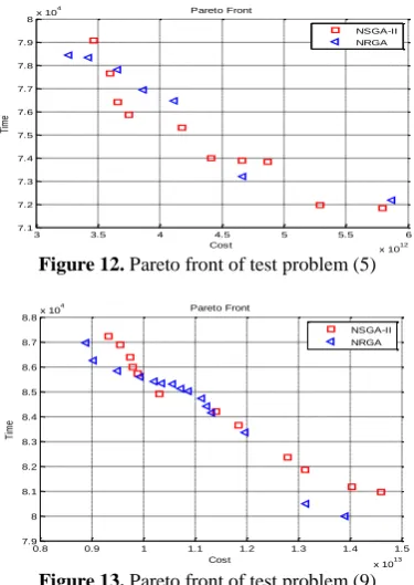
We note that while in terms of the SNS and NPS metrics, bigger values are desired, for spacing, MID and CPU time, smaller values are better. Then, in general, based on the outputs in the last row of Table 8, it is clear that NSGA-II shows better performances in terms of SNS and CPU time. Meanwhile, for other two metrics, NPS and MID, MRGA has better performances. Besides, to clarify better performance of the proposed Pareto-based algorithms, the obtained Pareto solutions of all algorithms on four test problem 1, 5, and 9 are presented in Figures 11-13.

Figure 11. Pareto front of test problem (1)

NRGA NSGA-II

13

12

11

10

9

Da

ta

Interval Plot of NPS

NRGA NSGA-II

3500

3000

2500

2000

1500

1000

500

0

Da

ta

Interval Plot of CPU Time

NRGA NSGA-II

4.25

4.00

3.75

3.50

3.25

3.00

2.75

2.50

D

at

a

Interval Plot of MID

NRGA NSGA-II

1.4000E+12

1.3000E+12

1.2000E+12

1.1000E+12

1.0000E+12

9.0000E+11

8.0000E+11

7.0000E+11

6.0000E+11

5.0000E+11

Da

ta

Interval Plot of SNS

2 2.5 3 3.5 4 4.5 5 5.5 6 6.5 7

x 1011 4.5

4.6 4.7 4.8 4.9 5 5.1 5.2 5.3x 10

4

Cost

Ti

m

e

Pareto Front

(11)

7. CONCLUSION

In this paper, a bi-objective mixed integer linear programming to specify the location of CWs and LDCs, simultaneously and the corresponding inventory quantities for relief items, and the distribution quantities from supplier to CWs, from CWs to the affected areas (LDC) and from strategic stock to LDC. The presented model seeks to minimize the cost variability, expected total cost. In the second stage, a relief distribution plan is extended based on different disaster scenarios by goals of minimizing the total distribution time, the maximum weighted distribution time of critical items, total cost of unused inventories, and the shortage cost of unmet demands. The model considers uncertainty in the locations where the demands might increase like as the possibility that some of the pre-arranged supplies at CWs or suppliers might be destroyed partially regarding to the disaster (i.e., supply uncertainty). To demonstrate the imprecise parameters, we make utilize of discrete scenarios from set S of potential disaster conditions. Then, in view of the NP-Hardness of proposed model, two tuned Pareto-based multi-objective meta-heuristic algorithms, called NSGA-II and NRGA were proposed to solve the problem.

Moreover, to achieve better performance, these algorithms are tuned by Taguchi method. The proposed algorithms were compared using 10 test problems via four multi-objective metrics. Also, to validate proposed framework, ɛ-constraint method is used in low dimension problems. Moreover, the perfomance of two algorithms for each matric via statistically method

called the intervals plot are analyzed. As is shown in Figure 11 and Table 8, two developed metaheuristics have a close behavior with ɛ-constraint method which refers to efficiency of these two algorithms. Finally, based on the results it was shown that: NSGA-II shows better performances in terms of SNS and CPU time, meanwhile, for NPS and MID, MRGA has better performances. Finaly, managers by using this comprehensive framework and solution approaches can achive the best performance includes minimum total costs and minimum of maximum travel time, and based on their organization directions can choose best solution among pareto fronts. As a limitation, it should be noted that the proposed framework and data are related to the selected case study and we cannot be sure that these outcomes will be efficient for other areas.

As future research, the model can be extended to have multiple fuzzy-objective. In addition, different methods for solving the proposed model can be developed. Applying the proposed model in similar fields can be one of the research areas for the future studies. The proposed solution approaches can also be used for the aforementioned cases.

8. REFERENCES

1. Galindo, G. and Batta, R., "Review of recent developments in or/ms research in disaster operations management", European Journal of Operational Research, Vol. 230, No. 2, (2013), 201-211.

2. Zokaee, S., Bozorgi-Amiri, A. and Sadjadi, S.J., "A robust optimization model for humanitarian relief chain design under uncertainty", Applied Mathematical Modelling, Vol. 40, No. 17, (2016), 7996-8016.

3. Boonmee, C., Arimura, M. and Asada, T., "Facility location optimization model for emergency humanitarian logistics",

International Journal of Disaster Risk Reduction, (2017). 4. Hoyos, M.C., Morales, R.S. and Akhavan-Tabatabaei, R., "Or

models with stochastic components in disaster operations management: A literature survey", Computers & Industrial Engineering, Vol. 82, (2015), 183-197.

5. Hristidis, V., Chen, S.-C., Li, T., Luis, S. and Deng, Y., "Survey of data management and analysis in disaster situations", Journal of Systems and Software, Vol. 83, No. 10, (2010), 1701-1714. 6. Caunhye, A.M., Nie, X. and Pokharel, S., "Optimization models

in emergency logistics: A literature review", Socio-economic Planning Sciences, Vol. 46, No. 1, (2012), 4-13.

7. Özdamar, L. and Ertem, M.A., "Models, solutions and enabling technologies in humanitarian logistics", European Journal of Operational Research, Vol. 244, No. 1, (2015), 55-65. 8. Sahebjamnia, N., Torabi, S.A. and Mansouri, S.A., "A hybrid

decision support system for managing humanitarian relief chains", Decision Support Systems, Vol. 95, No., (2017), 12-26.

9. Yazdani, A. and Kowsari, M., "Statistical prediction of the sequence of large earthquakes in iran", International Journal of Engineering-Transactions B: Applications, Vol. 24, No. 4, (2011), 325-333.

10. Nateghi, F., Dehghani, A. and Tabnak, A., "Seismic damage and disaster management maps (a case study)", International Journal of Engineering-Transactions B: Applications, Vol. 21, No. 4, (2008), 337-343.

3 3.5 4 4.5 5 5.5 6

x 1012

7.1 7.2 7.3 7.4 7.5 7.6 7.7 7.8 7.9

8x 10

4

Cost

Ti

m

e

Pareto Front

NSGA-II NRGA

0.8 0.9 1 1.1 1.2 1.3 1.4 1.5

x 1013

7.9 8 8.1 8.2 8.3 8.4 8.5 8.6 8.7 8.8x 10

4

Cost

Ti

m

e

Pareto Front

(12)

11. Rajabipour, A. and Behnamfar, F., "A fire ignition model and its application for estimating loss due to damage of the urban gas network in an earthquake", International Journal of Engineering, Transactions B: Applications, Vol. 29, No. 11, (2016), 1507-1519.

12. Yazdani, A., Shahpari, A. and Salimi, M., "The use of monte-carlo simulations in seismic hazard analysis in tehran and surrounding areas", International Journal of Engineering-Transactions C: Aspects, Vol. 25, No. 2, (2012), 159-166. 13. Aksen, D. and Aras, N., "A bilevel fixed charge location model

for facilities under imminent attack", Computers & Operations Research, Vol. 39, No. 7, (2012), 1364-1381.

14. Chang, M.-S., Tseng, Y.-L. and Chen, J.-W., "A scenario planning approach for the flood emergency logistics preparation problem under uncertainty", Transportation Research Part E: Logistics and Transportation Review, Vol. 43, No. 6, (2007), 737-754.

15. Chanta, S. and Sangsawang, O., "Shelter-site selection during flood disaster", Lect. Notes Manag. Sci, Vol. 4, (2012), 282-288.

16. DAS, R. and HANAOKA, S., "Robust network design with supply and demand uncertainties in humanitarian logistics",

Journal of the Eastern Asia Society for Transportation Studies, Vol. 10, (2013), 954-969.

17. Dekle, J., Lavieri, M.S., Martin, E., Emir-Farinas, H. and Francis, R.L., "A florida county locates disaster recovery centers", Interfaces, Vol. 35, No. 2, (2005), 133-139.

18. Dessouky, M., Ordonez, F., Jia, H. and Shen, Z., "Rapid distribution of medical supplies", International Series in Operations Research and Management Science, Vol. 91, (2006), 309-318.

19. Feng, C. and Wen, C., "A bi-level programming model for allocating private and emergency vehicle flows in seismic

disaster areas", in Proceedings of the Eastern Asia Society for Transportation Studies, Vol 5. Vol. 5, (2005), 1408-1423. 20. Hong, J.-D., Xie, Y. and Jeong, K.-Y., "Development and

evaluation of an integrated emergency response facility location model", Journal of Industrial Engineering and Management, Vol. 5, No. 1, (2012), 4-12.

21. Jabbarzadeh, A., Fahimnia, B. and Seuring, S., "Dynamic supply chain network design for the supply of blood in disasters: A robust model with real world application", Transportation Research Part E: Logistics and Transportation Review, Vol. 70, No., (2014), 225-244.

22. Kedchaikulrat, L. And Lohatepanont, M., "Multi-objective location selection model for thai red cross’s relief warehouses", in Proceedings of the Eastern Asia Society for Transportation Studies. Vol. 10, (2015).

23. Cheraghalipour, A. and Hajiaghaei-keshteli, M., "Tree growth algorithm (TGA): An effective metaheuristic algorithm inspired by trees behavior", in 13th International Conference on Industrial Engineeringn, Scientific Information Databases., (2017), 1-8.

24. Cheraghalipour, A., Paydar, M.M. and Hajiaghaei-keshteli, M., "“An integrated approach for collection center selection in reverse logistics", International Journal of Engineering, Transactions A: Basics, Vol. 30, No. 7, (2017), 1005-1016. 25. Deb, K., Pratap, A., Agarwal, S. and Meyarivan, T., "A fast and

elitist multiobjective genetic algorithm: NSGA-II", IEEE Transactions on Evolutionary Computation, Vol. 6, No. 2, (2002), 182-197.

26. Al Jadaan, O., Rajamani, L. and Rao, C., "Non-dominated ranked genetic algorithm for solving multi-objective optimization problems: NRGA", Journal of Theoretical & Applied Information Technology, Vol. 4, No. 1, (2008). 27. Taguchi, G., "Introduction to quality engineering: Designing

quality into products and processes, (1986).

A Bi-objective Stochastic Optimization Model for Humanitarian Relief Chain by

Using Evolutionary Algorithms

N. Javadiana_{, S. Modarres}a_{, A. Bozorgi}b

a_{Mazandaran University of Science and Technology, Mazandaran, Iran}

b_{School of Industrial Engineering, College of Engineering, University of Tehran, Tehran, Iran}

P A P E R I N F O

Paper history:

Received 07 March 2017

Received in revised form 21 June 2017 Accepted 07 July 2017

Keywords: Lines of Code Uncertainty ɛ-constraint Method Emergency Logistics Humanitarian Relief Chain Evolutionary Algorithm

ديكچ ه

یدادما هریجنز عوضوم ،یتسیرورت تلامح و گنج دننام یعیبط ریغ یایلاب و لیس و هلزلز دننام یعیبط یایلاب نازیم شیازفا هب هجوت اب هتفرگ رارق اهروشک زا یرایسب رظن دروم هناتسودرشب تسا

.

ربانب مدع تحت هناتسود رشب یدادما هریجنز هب کمک هلاقم نیا فده ،نیا

یلحم عیزوت زکارم لماش هناتسودرشب کیتسجل هکبش یحارط هلاسم کی ،شهوژپ نیا رد .دشاب یم تیعطق

(LDC)

یزکرم اهرابنا و

ددعتم

(CWS)

( ویرانس رب ینتبم یفداصت درکیور کی هعسوت و

SBSP

و اضاقت اب طابترا رد تیعطق مدع ،نینچمه .تسا هدش هئارا )

یزاس هنیهب هئارا اب هلزلز زا دعب لقن و لمح هکبش یاهریسم حوطس ندوب سرتسد رد زین و نیمات تاعلاطا یعطقریغ

هدش هتفرگ رظن رد