An Inventory Model for Deteriorating Items Using Vendor-Managed Inventory Policy

Please cite this article as: M. Setak, L. Daneshfar, An Inventory Model for Deteriorating Items Using Vendor-Managed Inventory Policy. International Journal of Engineering (IJE) Transactions A: Basics, Vol. 27, No. 7, (2014): 1081-1090

International Journal of Engineering

J o u r n a l H o m e p a g e : w w w . i j e . i r

An Inventory Model for Deteriorating Items Using Vendor-Managed Inventory

Policy

M. Setak*, L. Daneshfar

Department of Industrial Engineering, K.N. Toosi University of Technology, Tehran, Iran

P A P E R I N F O

Paper history:

Received 26 September 2013

Received in revised form 02 November 2013 Accepted 07 November 2013

Keywords:

Vendor-managed Inventory (VMI) Deterioration

Stock-dependent Demand Partial Backlogging

A B S T R A C T

In recent researches, vendor managed inventory (VMI) policy is rarely considered in the case of deteriorating items. This study considers the supply chain partner’s collaboration via a VMI system and provides an EOQ model for a two-level supply chain (single supplier-single retailer) with stock-dependent demand and constant deterioration and backlogging rates, to examine the inventory management proceedings for VMI and non-VMI supply chains. The equations are simplified using a new approach in modeling. A comparison between the costs of two mentioned cases is done. The results of analytical examination of inventory costs with and without VMI show that VMI system in our proposed model always has the ability to reduce total costs of the supply chain and is always better than the traditional one. Some numerical examples and sensitivity analysis are also given to illustrate the application of the proposed model.

doi:10.5829/idosi.ije.2014.27.07a.09

1. INTRODUCTION1

In traditional supply chain strategies, each party in the chain focuses on its own profit. Hence, decisions are made with little regard to their impact on other supply chain partners. Vendor Managed Inventory (VMI) is a streamlined approach to inventory management and order fulfillment. VMI involves collaboration between suppliers and their customers (e.g., distributor, retailer, or product end user) which changes the traditional ordering process.The emergence of a VMI system goes back to 1980s [1] and nowadays the usage of VMI has become more vital [2]. Supply chain performance will improve in the light of a VMI system because of its reduction in inventory levels [3]. The purpose of its partnership is to share information between members of the supply chain resulting in shorter lead times, reduced inventory, reduced obsolescence, and more efficient manufacturing. The up-stream member of the supply chain (the supplier) takes on more decision making for what to supply to the customer. The result is a more leveraged relationship for the supplier and improved service for the customer [4].

1_{*Corresponding Author’s Email: [email protected] (M. Setak)}

In the overall deterioration means: decay, damage, evaporation, obsolescence or loss of product value over the time [5]. Deterioration in many inventory systems such as food items plays an important role. Food retailers, such as Kraft Foods, Wal-Mart, McCain Foods and Barilla continuously deal with deteriorating products. One of the most advantages of VMI implementation are to provide their retailers and end consumers with foods with their best initial quality and freshness [1]. In this paper, we have extended Pasandideh’s model [6] by formulating an EOQ model for deteriorating items with stock dependent demand and partial backlogging and using different approaches in modeling and the way of simplifying the equations used by Pentico and Drake [7]. The model considered for a two-level supply chain consists of one supplier- one retailer to evaluate the inventory control costs before and after implementing VMI system. The rest of the paper is structured as follows: the next section, reviews the related literature in two scopes: VMI and deteriorating items. Section 3 describes the proposed model framework, and contains the model, its assumptions and notations. Section 4 analyzes cost savings due to VMI by an inverted procedure. To explain the application of our model, three numerical

examples and related analysis are given in Section 5. The paper ends with conclusions and some suggestions for future research, in section 6.

2. LITERATURE REVIEW

Inventory problems in VMI supply chains have been widely studied for non-deteriorating items [1]. By probing and searching in existing literature, although extremely limited, it is clear that VMI especially before the second half of the 90th _{century was considered not as} a basis for inventory management but as a flavoring in inventory management.A conceptual framework of VMI was explained by Magee [8] while discussing about the responsibility for inventory control.But from the second half of the 90th _{century, with the introduction of internet} technology, the VMI was not more looked as an unreachable ideal, while the impact of this change in attitude is clearly seen in the literature.VMI is widely studied by many researchers [9] where suppliers try to sync their cycles of production with their retailers’ orders by expressing a common replenishment cycle. Dong and Xu [10] assessed how VMI policy impacts a supply chain and showed the VMI is an impressive strategy that can realize many of the advantages achievable only in a totally integrated supply chain. Yao et al. [11] also developed an analytical model and demonstrated the benefits, as inventory cost reductions, may be appeared from integration according to the ratio of the order costs of the supplier to the buyer and the ratio of the carrying charges of the supplier to the buyer. They also showed that how the benefits are likely to be distributed between buyers and suppliers. Van Der Vlist et al. [12] developed the Yao et al. [11] model by considering shipping costs from the supplier to the buyer. Pasandideh et al. [6] developed a model to discover the effect of main supply chain parameters on the cost savings with the use of VMI policy. Yugang et al. [1] considered a VMI supply chain for products and raw materials where both are deteriorating items.In recent years, most researches in the area of inventory control have been oriented towards the development of more realistic and practical models for decision makers. Recently, deteriorating of items in inventory system has become an interesting topic due to its practical importance [13]. It should be considered that deteriorated products in developing the models, in comparison with non-deteriorating items, are more complicated. To date, in many researches, the deterioration of items has been considered which represents the importance of deterioration in inventory problems. Whitin [14] was the first onewho considered deterioration, such asfashion items deteriorating. Ghare and Schrader [15] established a model for an exponentially decaying inventory. Inventory models with time dependent deterioration were established by

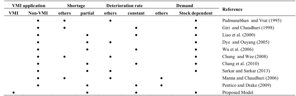
TABLE 1. Classified viewed articles

VMI application Shortage Deterioration rate Demand

Reference VMI Non-VMI others partial others constant others Stock dependent

● ● ● ● Padmanabhan and Vrat (1995)

● ● ● ● Giri and Chaudhuri (1998)

● ● ● ● Liao et al. (2000)

● ● ● ● Dye and Ouyang (2005)

● ● ● ● Wu et al. (2006)

● ● ● ● Chung and Wee (2008)

● ● ● ● Chang et al. (2010)

● ● ● ● Sarkar and Sarkar (2013)

● ● ● ● Manna and Chaudhuri (2006)

● ● ● ● Pentico and Drake (2009)

● ● ● ● Proposed Model

3. MODELING

3. 1. Problem Deinition We considered a two level supply chain (single supplier-single retailer) that acts under VMI and non-VMI policy. In an integrated supply chain, the supplier receives the details of the customer demand directly. Therefore, the supplier is now responsible for all the deterioration, shortage, ordering and holding cost.That means the supplier inventory cost equals to the total integrated supply chain cost, therefore according to the total cost, determines the timing and the quantity of replenishment in every cycle. The main difference between a VMI and traditional system is that in a VMI system, this is the supplier that determines the retailer order quantity [26].Next, the assumptions and notations whichhave been used are provided:

3. 2. Assumptions The following assumptions are used:

1. A single-supplier–single-retailer supply chain with one item is considered.

2. Lead time is zero.

3. The planning horizon is infinite.

4. The demand rate R(I(t)) is known as a function of instantaneous stock level I(t);R(I(t)) is taken as following form:

î í ì

£ > +

=

0 I(t) if

0 I(t) if ) ( ))

( (

D t I D t I

R a

5. The on hand inventory deteriorates at a constant rate θ (0 <θ <1) per time unit.

6. There is no repair or replacement of the deteriorated items.

7. The shortage is allowed and partially backlogged. 8. β is the backlogging rate and is constant; 0<β<1.

3. 3. Notations

AS Supplier's ordering cost per cycle AR Retailer 's ordering cost per cycle P Purchase cost per unit

θ The deterioration rate

H The holding cost per unit per unit time S The shortage cost per unit per unit time

l The lost sale cost due to lost sales per unit per unit time

I(t) The inventory level at time t, where tÎ_{[0, ]}T

β The backlogging rate and is constant; 0£ £b 1 T The length of the replenishment cycle

K The percentage of the cycle that inventory is positive; 0≤ K ≤1

Q Order quantity per cycle

TCRVMI Retailer 's inventory cost after VMI TCSVMI Supplier's inventory cost after VMI TCVMI Total costs of VMI supply chain TCRnoVMI Retailer's inventory cost before VMI TCSnoVMI Supplier's inventory cost before VMI TCnoVMI Total costs of non-VMI supply chain

3. 4. Decision Variables

T Common replenishment cycle for the vendor to replenish the product to the retailer

K The percentage of the cycle that inventory is positive; 0≤ K ≤1

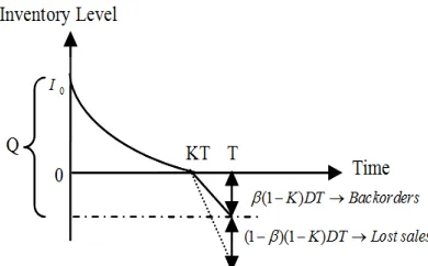
Figure 1. The inventory level of the product in a cycle

As shown in Figure 1, at the beginning of the cycle the inventory is maximum, then the inventory level decreases due to demand and deterioration up to t=KT. At this time inventory reaches zero and shortage is occurring and is partially backordered during [KT,T]. At the end of the cycle, the inventory reaches the maximum backordered level. So as described, the changes of inventory at evrywhere are shown using the two following differential equations:

1

1 1 1 1

( )

( ) ( ( )) ( ) ( ) ( ) ( )

; 0 t KT

dI t

I t R I t I t I t D I t

dt D

q q a q a

= - - = - - - = +

- £ £ (1)

T t KT ; ) (

2 _{=- D £ £}

dt t

dI _b

(2)

With the boundary condition I(t)=0; t=KT, the solutions of the above differential equations (1) and (2) areobtained as the following equations:

KT t 0 ); 1 ( ) ( ( )( )

1 = ₊ - £ £

-+ KT t e D t

I q a

a

q (3)

T t KT ); ( ) (

2 t =- D t- KT £ £

I b (4)

3. 5. 1. The Case of VMI Supply Chain In a VMI system, some agreements are made between the parties. First, supplier determines the timing and order quantity of each period, second in addition to its own ordering cost, takes full responsibility for all the inventory and ordering cost of the retailer.

After implementing the VMI, the inventory costs of the retailer and supplier and, thus, the total inventory costs of the VMI supply chain are computed as follows [26]:

0 TCRVMI =

HC) LC SC PC A (A 1

TCSVMI= S+ R+ + + +

T (5)

TCS T

K) (T,

TCVMI = CRVMI+ VMI (6)

where

AS + AR Ordering cost per cycle

PC Total purchase cost per cycle

SC Total backordered cost per cycle

LC Total lost sale cost per cycle

HC Total holding cost per cycle

So the total purchase cost is calculated as follows:

] K)T -D(1 1) -(e D P[ K)T -D(1 (0) p[I PQ

C ( )( )

1 b _{q a} b

a q ₊ + = + =

= + KT

P (7)

Using the Taylor expansion:

2 2 2 ) )( ( _{( )} 2 1 ) (

1 KT K T

eq+a KT _{= + q +a + q +a (8)}

So ) 1 ( 2 ) ( PDK PDKT C 2 2 K T PD T

P = + q +a + b - (9)

and its backordered cost per cycle is:

2 2 2() ( ) ₂ (1 K)T

D S dt KT t D S dt t I S SC T KT T KT -= -=

-= _{ò ò}b b (10)

and the lost sale cost due to lost sales per cycle is:

DT K l Ddt l dt t I R l L T KT T KT ) 1 )( 1 ( ) 1 ( )) ( ( ) 1

(- 1 = - = -

-= _ò b _ò b b (11)

Finally, the total inventory holding cost in a common replenishment cycle is given as:

( )( )

1 2

0 0

( )( )

( ) ( 1)

( ) ( )

( 1 ( ) )

KT KT

KT t

KT

hD hD

HC hI t dt e dt

KT e

q a

q a

q a q a

q a + -+ = = - = + + - - + +

ò

ò

₍₁₂₎

By usingthe Taylor expansion and simplifying we have:

2

2 2_T hDK

HC= (13)

Therefore,the total cost of the inventory system during the period [0, T] is given by:

2 2 2 2 2 ( , ) 1 1 ( , ) ( ) ( ( )

(1 ) (1 )

2 2

(1 )(1 ) )

2 VMI VMI VMI

VMI S R S R

TC T K TCR TCS

TC T K A A PC SC LC HC A A

T T

PDK T S D

PDKT PD T K K T

hDK T

l K DT

q a _b b

b = + ® = + + + + + = + + + + + - + -+ - - + (14)

By simplifying the total cost function, we have:

b b b b b b a q b PD D l PD PD D l K D S D S K pD D S hD K T A A T K T

TCVMI S R

+ -+ + -+ -+ + + + + = ) 1 ( ] ) 1 ( [ ] 2 ) 2 ( 2 ) 2 ) ( ( [ ] [ 1 ) , ( 2 (15)

By simplifications used by Pentico and Drake [16] in equations, TCVMI(T,K) can be rewritten as:

2 0

1 2 2 3 4

( , ) [ 2 ]

VMI

W

TC T K T K W KW W KW W

T

where b b b b b b a q b PD D l W P l D PD PD D l W D S W pD D S hD W A A

W _{S R}

+ -= -= + -= = + + + = + = ) 1 ( ) )( 1 ( ) 1 ( 2 2 ) ( 4 3 2 1 0

Because all parameters are positive, hence allW0, W1, W2 and W4 are positive except W3, that depends on the parameters P and l and are considered as W1>W2. Our objective is to create conditions under which Equation (16) has a unique interior which minimizes the cost function.

The optimum values of decision variables (T*, K*) could be obtained by getting the first derivations of the cost function with respect to decision variables and setting them to zero.

By first derivation of TCVMI(T,K) with respect to T and setting it zero we get:

0 ] 2 [ ) , ( 2 2 1 2

20+ - + =

-= ¶

¶ _{KW KW W}

T W T K T TCVMI (17)

The above phrase equals zero only when T satisfies:

2 2 1 2 * 2 0 ) ( W KW W K W K TVMI + -= (18) Then, 2

1 2 2

( ) 2

y K =K W - KW +W

Because the discriminatorof y(K),

2

2 1 2 2 2 1

( 2 )W 4WW 4 (W W W)

D = - - = - is negative, y(K)does not have any root. Thus, y K( )does not equal to zero and is positive or negative. Since, y(0)= W2>0, so y(k) is positive.

So, Equation (18) for each K gives an exclusive T

that minimizes the cost function given by Equation (16). At the same time, getting first derivation ofTCVMI(T,K) with respect to K and setting it as zero results in:

0 ] 2 2 [ ) , ( 3 2

1- - =

= ¶ ¶ W W KW T K K T

TCVMI ₍₁₉₎

1 2 3 * 2 2 ) ( W W T W T K VMI + = (20)

With respect to Equation (20),we conclude that the decision variable “K” has a unique quantity; and If “K” in the interval [0 , 1] does not satisfy Equation (20), that means the cost function in Equation (16) is strictly increasing or decreasing at the range 0≤ K ≤1, thus the optimal value of “K” occurs at the corners, therefore: K*

VMI =0 or K*VMI =1.

By inserting Equation (20) into Equation (18), we have:

0

3 3

2 2

2

1 2 2

1 1

2 2

2

0 1 0 1

2 2 2 2 2 2

3 1 2 2 3 1 2 2

2 2 2

0 1 3 1 2 2

2

* 0 1 3

2

1 2 2

2 2

( ) 2( )

2 2

4 4

(4 4 ) (4 4 )

4 (4 4 )

4

4 4

VMI

W

T _{W W}

W W

T _W T _{W W}

W W

W WT _T W WT

W T WW W W T WW W

W W W T WW W

W W W T WW W = = + + - + ® = + - + -® = + - ® -= -(21)

And by substituting Equation (21) into Equation (20) we get: 1 2 2 2 2 1 2 3 1 0 3 * 2 2 4 4 4 W W W W W W W W W K VMI + -= (22)

Thus, optimum values of decision variables (T* VMI, K*VMI) are obtained by Equations (21) and (22).

To prove the convexity of the cost function given by Equation (16), first the second derivatives of TCVMI(T,K) is taken with respect to K:

0 2 ) , ( 1> = ¶ ¶ TW K K T

TCVMI ₍₂₃₎

This is positive for all T.

Then, inserting Equation (20) into Equation (16) results in:

3 3

2 2

* 0 2

1 2 1 1 2 3 3 ₀ 2 * 1

2 3 4

1 2 2 3 2 2 4 1 1 2 2

( , ) [( ) 2( )

2 2 ( ) 2 ₄ ] ( ) ( , ) 2 [ ] VMI VMI VMI VMI W W W W

W _{T T}

TC T K T W W

T W W

W

W _{W W}

W T

W W W TC T K

W T

W W W

T W W

W W + + = + -+ + - + ® = + - + -(24)

Since the only remaining decision variable in the cost functionTCVMI(T,K*VMI) is T, the partial differentiates with respect to T should be taken.

First derivation: 2 3 0 * 2 1 2 2 2 1 2 3 0 2

* 1 0 1 3

2 2

2 1 2 2

2 1

( )

( , ) 4

( ) 0

4 4 4 4 VMI VMI VMI W W

TC T K W W

W

T T W

W W

W W W W

T

W WW W

W W - -¶ _{= + - =} ¶ -® = = -(25)

That is the same as Equation (21). Second derivation:

31 2 3 1 0 3 1 2 3 0 2 *

2 ₄ )

4 ( 2 ) 4 ( 2 ) , ( T W W W W T W W W T K T

TCVMI VMI

-= -= ¶ ¶ (26)

Since the above condition holds, it can be concluded that the cost function is convex at the global optimum point (T*

By substituting Equations (21) and (22) into Equation (16) we obtain the following phrase for TCVMI(T*VMI, K* VMI): 1 3 2 4 1 2 2 2 1 2 3 0 * * _{)( )} 4 ( 2 ) , ( W W W W W W W W W W K T

TCVMI VMI VMI = - - + - (27)

Which represents the value of the objective function at the optimal point.

3. 5. 2. The Case of Traditional Supply Chain Before implementing VMI, there is no responsibility for supplier and the product enters directly to the retailer’s warehouse, thus all inventory costs will be borne by the retailer.

In this case, this is the retailer that determines the optimal timing and quantity replenishment in each cycle and the supplier just have to deliver the identified amount of products at the time scheduled by retailer.

The retailer determines the timing and quantity replenishment according to its own inventory costs which are not necessarily optimal and do not minimize the total cost function. In this case the retailer and supplier and thus the total cost function are calculated as follows (by using the simplified phrases):

2 0

1 2 2

3 4

( , ) S [ 2 ]

noVMI

W A

TC R T K T K W KW W

T KW W

-= + - +

- + (28)

( , ) S

noVMI

A TCS T K

T

= (29)

2 0

1

2 2 3 4

( , ) ( , ) ( , ) [

2 ]

noVMI noVMI noVMI

W

TC T K TCR T K TCS T K T K W

T

KW W KW W

= + = +

- + - + (30)

By getting the partial differentiates of TCnoVMI(T,K) with respect to decision variables respectively and setting them to zero we get:

2 0 1 2 2 ( , ( ) ) 2 0

no VM I S

TC R T K W A

K W K W

T T

W

¶ -

-= +

-¶

+ = (31)

* 0

2

1 2 2

( )

2 S n oVM I

W A

T K

K W K W W

-® =

- + (32)

As proved before, sincey(K)is all positive, thus Equation (32) for each K, gives an exclusiveTthat minimizes the cost function given by Equation (28).

1 2 3

( , )

[ 2 2 ] 0

noVM I

TC R T K _{T K W W W} K ¶ _{= - - =} ¶ (33) 3 2 * 1 2 2 noVMI W W T K W + = (34)

As before, with respect to Equation (34) we conclude that the decision variable “K” has a unique quantity; and

if “K” in the interval [0 , 1] does not satisfy Equation (34), that means the cost function in Equation (28)is strictly increasing or decreasing at the range 0≤K≤1, thus the optimal “K” occurs at the corners, therefore: K*

noVMI=0orK*noVMI=1. By inserting Equation (34) into Equation (32), we have:

0

3 3

2 ₂ 2

1 2 2

1 1

2

0 1

2 2 2

3 1 2 2

2 2

( ) 2 ( )

2 2

4 ( )

( 4 4 )

S

S

W A

T

W _W W _W

T _W T _{W W}

W W

W A W T

W T W W W

-= = + + - + -+ -2

2 0 1 2

0 1 3

2 2 2

3 1 2 2

2 2

1 2 2

4( )

4( ) (4 4 )

(4 4 ) S

S

W A WT

T W A W W

W T WW W

T WW W

-® = ® - = +

+

-2

* 0 1 3

2

1 2 2

4( )

(4 4 )

S noVMI

W A W W

T

WW W

-

-® =

- (35)

and by inserting Equation (35) into Equation (34), we have:

Thus, the optimal values of decision variables (T* noVMI, K*

noVMI) are obtained by Equations (35) and (36). To prove the convexity of the cost function given by Equation (28), first the second derivativeof TCRnoVMI(T,K) is taken with respect to K:

1

( , ) _{2 0}

noVMI

TCR T K _TW K

¶

= >

¶ (37)

which is positive for all T.Then, inserting Equation (34) into Equation (28) results in:

3 2

* 0 2

1 1

3 3

2 2

2 2 3 4

1 1

2 3

0 2

* 1 2 2 3

2 4 1 1 2 ( , ) [( ) 2 2 2

2( ) ] ( )

2 2 4 ( , ) [ ] S noVMI noVMI S noVMI noVMI W W

W A _T

TCR T K T W

T W

W _W W _W

T _{W W} T _{W W}

W W

W

W A

WW

W W

TCR T K T W W

T W W

+ -= + -+ + + - + ® - -= + - + -(38)

Since the only remaining decision variable in the cost function TCVMI(T, K*VMI) is T, the partial differentiates with respect to T should be taken.

First derivation: 0 ) ( ) 4 ( ) , ( 1 2 2 2 2 1 2 3 0 * = -+ -= ¶ ¶ W W W T W W A W T K T TCR S noVMI noVMI 2 2 2 1 2 3 1 0 1 2 2 2 1 2 3 0 * 4 4 ) ( 4 4 W W W W W A W W W W W W A W T S S noVMI -= -=

® (39)

3

2 2

0 1 3

2

1 2 2

*

1 2

4( )

(4 4 )

2

S

noVMI

W

W W A W W

That is the same as Equation (35).Second derivation:

2 2

3 0 1 3

0

2 *

1 1

2 3 3

4( )

2( ) 2( )

( , ) 4 4

0

S S

noVMI noVMI

W W A W W

W A

TCR T K W W

T T T

- --

-¶ _{= = >}

¶ (40)

Since the above condition holds, it can be concluded that the cost function is convex at the global optimal point (T*

noVMI, K*noVMI).

By substituting Eequations (35) and (36) into Equation (30) we obtain the following phrase for TCnoVMI(T*noVMI, K* noVMI): 1 3 2 4 1 2 3 0 1 2 3 0 1 2 3 0 1 2 2 2 * * ) 4 ( ) 4 ( ) 4 ( ( ) ( ) , ( W W W W W W A W W W A W W W W W W W K T TC S S noVMI noVMI noVMI -+ -+ -= (41)

That represents the value of the objective function at the optimal point.

4. COMPARISON OF TWO CASES: VMI AND NON-VMI SUPPLY CHAIN

To compare and analyze the total inventory costs before and after implementation of VMI in the supply chain, we establish the following assumption and by an inverted procedure we reach the appropriate condition that the inequality holds:

) , ( ) , ( * * * * noVMI noVMI noVMI VMI VMI

VMI T K TC T K

TC £ (42)

2 3 0

2 2 2

3 2 2 3 2 1

0 2 4 2 ₂

1 1 1 1 3

0 1 2

3 2 3

0 4

1 1

4

2 ( )( ) ( ) ( )

4 ( ) 4 ( ) 4 S S W W

W W W W W W

W W W W

W W W W _{W A} W

W

W W W

W A W

W W -® - - + - £ -- -+ - - + -) 4 ( ) 4 ( 4 ) 4 ( 2 ) 4 ( ) ) 4 ( 4 ( ) ( ) )( 4 ( 2 ) , ( ) , ( 1 2 3 0 1 2 3 0 1 2 3 0 1 2 3 0 1 3 2 4 1 2 3 0 1 2 3 0 1 2 3 0 1 2 2 2 1 3 2 4 1 2 2 2 1 2 3 0 * * * * W W A W W W A W W W W W W W W W W W W W A W W W A W W W W W W W W W W W W W W W W W K T TC K T TC S S S S noVMI noVMI noVMI VMI VMI VMI -+ -£ -® -+ -+ -£ -+ -® £

By above simplifications we reach the following condition: ) 4 ( ) 4 ( 4 ) 4 ( 2 1 2 3 1 2 3 1 2 3 1 2 3 W W A W W A W W A A W W A A R R R S R

S +

-+ £ -+

® ₍₄₃₎

If we set

) 4 ( ) 4 ( 4 ) 4 ( 2 ) ( 1 2 3 1 2 3 1 2 3 1 2 3 W W A W W A W W A A W W A A A U R R R S R S

S -

-+ -+ = ® ₍₄₄₎

By getting the first derivation ofU(AS) with respect to ASwe have:

0 0 ) 4 ( 1 ) 4 ( 1 ) ( 1 2 3 1 2 3 = ® = -+ = ¶ ¶ ® S R R S S S _A W W A W W A A A A U (45)

Thus the above equation gets zero at AS =0and for AS>0, is all negative. Thus U(AS) is decreasing due to

S

A and is maximum at the point AS =0: 2 3

2 2 2

3 1 3 3

2

1 3 1 1

1

0 4

( 0) 2 (0 ) ( ) 2 ( )

4 4 4

( )

4 R

S R R R

R

W A

W W W W

U A A A A

W _W W W

A W + -= = + - - - - = -2 3 2 3 1 2 1 3 1

4 _{( ) 0}

4 ( ) 4 R R R W A W W A W W A W -- - - =

-That equals zero (means total costs are the same in VMI and traditional supply chain) and because it is a decreasing function, so it becomes negative for all other AS as shown in Figure 2. So the condition given by Inequality (44) always holds; and we can conclude that in the proposed model, (i) implementing VMI decreases total costs of the supply chain, and (ii) VMI system is always better than the traditional one.

Figure2. Display U(AS ) versus AS

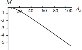
Figure 4. Display M function versus AS

5. NUMERICAL EXPERIMENTS AND SENSITIVITY ANALYSIS

In order to explain the application of the mentioned model and evaluate the comparison, three numerical examples and related analysis are given.

5. 1. Numerical Examples The values for the parameters are shown in Table 2, such that all parameters are constant and the values related to P are different in the examples.The results of the examples are gathered in Table 3 and the performance of the VMI system is obvious.The cost function of example 1 is shown in Figure 3.

5. 2. Sensitivity Analysis To evaluate the effect of changes in model parameters on total cost in two

mentioned cases with increasing or decreasing the parameter AS and keeping the other parameters without any change, sensitivity analysis is done and the related results are shown in Table 4 and Figure 4. Also we analyzed the changes in cost functions with increasing or decreasing the parameters αand θas the main parameters of our model and showed the results at the end of Table 4. By forming M function and observing the values obtained from changing in parameterASin Table 4, it can be seen thatthe VMI system is always better than the traditional one; andasshown in Figure 4 with an increase in the parameterAS, VMI system causes greater reduction in supply chain costs. Also it is obvious that by any change in the main parameters, VMI is better than non-VMI system; and with increase in the parameters α and θ,the cost of both cases will increase but the absolute valueofthe difference betweenVMI and non-VMI costs (Mvalue) will decline slightly.

TABLE 2. The initial data of numerical examples

Example AS AR D h P l S q a β

Example1 70 30 200 2 8 12 3 0.1 0.6 0.8 Example2 70 30 200 2 12 12 3 0.1 0.6 0.8 Example3 70 30 200 2 15 12 3 0.1 0.6 0.8

TABLE 3. The results of three examples

Example K*VMI T*VMI TC*VMI Q*VMI K*noVMI T*noVMI TC*noVMI Q*noVMI _TC*_noVMI-TC*_noVMI

Example1 0.352 0.7163 1982.92 129.409 0.46 0.359 2047.42 66.219 -64.5

Example2 0.187 0.7161 2679.28 121.252 0.187 0.392 2731.44 66.084 -52.16

Example3 0.103 0.696 3179.67 114.631 0.052 0.370 3237.5 60.022 -57.83

TABLE 4. Results for sensitivity analysis

Parameter A=TC_VMI(T*VMI,K*VMI) B=TCnoVMI(T*noVMI,K*noVMI) M=100((A-B)/A)

0 1852.82 1852.82 0

10 1878.17 1880.62 - 0.1304%

AS 30 1919.35 1936.22 - 0.8788%

50 1953.33 1991.82 - 1.9707%

100 2091.9 2130.83 - 5.3875%

0.3 1954.73 2077.84 -6.2981%

α 0.45 1970.81 2093.5 -6.2254%

0.75 1992.39 2114.51 -6.1293%

0.9 2000 2121.91 -6.0955%

0.05 1979.23 2101.7 -6.1878%

θ 0.075 1981.12 2103.54 -6.1793%

0.125 1984.66 2106.99 -6.1638%

6. CONCLUSION AND FUTURE RESEARCH

This paper is an extension of Pasandideh’s model [6] by formulating an EOQ model for deteriorating items with stock dependent demand and partial backlogging in a two level supply chain. However, in most papers, the computations are difficult and some complicated, but in the above model, the calculations are facilitated using some simplifications in the equations. The type of objective function is cost and is minimized. Because of inability in proving the convexity of the cost function in general, we proved it is convex at the optimum point and because the answers for parameters K and T are unique, so the point(T*_{, K}*_{)is the global optimum.} At last by calculating the model, the optimal cycle time (T*_{), order quantity and the other decision variable} (K*_{)have been found. Also in the comparison between} VMI and non-VMI supply chain costs for the proposed model, we conclude that:

(i) implementing VMI decreases total costs of the supply chain, and

(ii) VMI system is always better than the traditional one.

As a result, for the same scenarios, we propose to use the VMI system.

In this research, modeling is done in a certain area and due to the complexity of stochastic areas, it was ignored; therefore, to improve the model, to get closer to reality, demand, lead time or the backlogging rate could be considered stochastic.

Also in the related inventory literature most researches assumed just one item, however in reality we face more than one item; hence the above model could be extended by considering two or more products.

Also by considering some constraints such as limitation on the storage capacity or on the number of orders, the model is gotten closer to the reality.

7.REFERENCES [1-26]

1. Yu, Y., Wang, Z. and Liang, L., "A vendor managed inventory supply chain with deteriorating raw materials and products",

International Journal of Production Economics, Vol. 136, No.

2, (2012), 266-274.

2. Arora, V., Chan, F.T. and Tiwari, M.K., "An integrated approach for logistic and vendor managed inventory in supply chain", Expert Systems with Applications, Vol. 37, No. 1, (2010), 39-44.

3. Emigh, J., "Vendor-managed inventory: Financial and business concepts in brief", Computerworld, Vol., No., (1999), 33-52. 4. Disney, S.M., Potter, A.T. and Gardner, B.M., "The impact of

vendor managed inventory on transport operations",

Transportation Research Part E: Logistics and Transportation

Review, Vol. 39, No. 5, (2003), 363-380.

5. Roy, A., Kar, S. and Maiti, M., "A deteriorating multi-item inventory model with fuzzy costs and resources based on two different defuzzification techniques", Applied Mathematical

Modelling, Vol. 32, No. 2, (2008), 208-223.

6. Pasandideh, S.H.R., Niaki, S.T.A. and Nia, A.R., "An investigation of vendor-managed inventory application in supply chain: The eoq model with shortage", The International

Journal of Advanced Manufacturing Technology, Vol. 49, No.

1-4, (2010), 329-339.

7. Pentico, D.W. and Drake, M.J., "The deterministic eoq with partial backordering: A new approach", European Journal of

Operational Research, Vol. 194, No. 1, (2009), 102-113.

8. Magee, J.F. and Boodman, D.M., "Production planning and inventory control", Vol., No., (1967).

9. De Toni, A.F. and Zamolo, E., "From a traditional replenishment system to vendor-managed inventory: A case study from the household electrical appliances sector", International Journal

of Production Economics, Vol. 96, No. 1, (2005), 63-79.

10. Dong, Y. and Xu, K., "A supply chain model of vendor managed inventory", Transportation Research Part E: Logistics and

Transportation Review, Vol. 38, No. 2, (2002), 75-95.

11. Yao, Y., Evers, P.T. and Dresner, M.E., "Supply chain integration in vendor-managed inventory", Decision Support

Systems, Vol. 43, No. 2, (2007), 663-674.

12. Van der Vlist, P., Kuik, R. and Verheijen, B., "Note on supply chain integration in vendor-managed inventory", Decision

Support Systems, Vol. 44, No. 1, (2007), 360-365.

13. Jain, M., Sharma, G. and Rathore, S., "Economic production quantity models with shortage, price and stock-dependent demand for deteriorating items", International Journal of

Engineering Transactions A Basics, Vol. 20, No. 2, (2007),

159.

14. Whitin, T.M., "Theory of inventory management, Princeton University Press, (1957).

15. Ghare, P. M. and Schrader, G. F., “An inventory model for exponentially deteriorating items”, Journal of Industrial

Engineering, Vol. 14, (1963), 238-243.

16. MISRA, R.B., "Optimum production lot size model for a system with deteriorating inventory", The International Journal Of

Production Research, Vol. 13, No. 5, (1975), 495-505.

17. Manna, S. and Chaudhuri, K., "An eoq model with ramp type demand rate, time dependent deterioration rate, unit production cost and shortages", European Journal of Operational

Research, Vol. 171, No. 2, (2006), 557-566.

18. Sarkar, B. and Sarkar, S., "An improved inventory model with partial backlogging, time varying deterioration and stock-dependent demand", Economic Modelling, Vol. 30, No., (2013), 924-932.

19. Liao, H.-C., Tsai, C.-H. and Su, C.-T., "An inventory model with deteriorating items under inflation when a delay in payment is permissible", International Journal of Production

Economics, Vol. 63, No. 2, (2000), 207-214.

20. Padmanabhan, G. and Vrat, P., "Eoq models for perishable items under stock dependent selling rate", European Journal of

Operational Research, Vol. 86, No. 2, (1995), 281-292.

21. Giri, B. and Chaudhuri, K., "Deterministic models of perishable inventory with stock-dependent demand rate and nonlinear holding cost", European Journal of Operational Research, Vol. 105, No. 3, (1998), 467-474.

22. Dye, C.-Y. and Ouyang, L.-Y., "An eoq model for perishable items under stock-dependent selling rate and time-dependent partial backlogging", European Journal of Operational

Research, Vol. 163, No. 3, (2005), 776-783.

23. Wu, K.-S., Ouyang, L.-Y. and Yang, C.-T., "An optimal replenishment policy for non-instantaneous deteriorating items with stock-dependent demand and partial backlogging",

International Journal of Production Economics, Vol. 101, No.

24. Chung, C.-J. and Wee, H.-M., "Scheduling and replenishment plan for an integrated deteriorating inventory model with stock-dependent selling rate", The International Journal of Advanced

Manufacturing Technology, Vol. 35, No. 7-8, (2008), 665-679.

25. Sana, S.S., "An eoq model for perishable item with stock dependent demand and price discount rate", American Journal

of Mathematical and Management Sciences, Vol. 30, No. 3-4,

(2010), 299-316.

26. Chang, C.-T., Teng, J.-T. and Goyal, S.K., "Optimal replenishment policies for non-instantaneous deteriorating items with stock-dependent demand", International Journal of

Production Economics, Vol. 123, No. 1, (2010), 62-68.

An Inventory Model for Deteriorating Items Using Vendor-Managed Inventory

Policy

M. Setak, L. Daneshfar

Department of Industrial Engineering, K.N. Toosi University of Technology, Tehran, Iran

P A P E R I N F O

Paper history:

Received 26 September 2013

Received in revised form 02 November 2013 Accepted 07 November 2013

Keywords:

Vendor-managed Inventory (VMI) Deterioration

Stock-dependent Demand Partial Backlogging

هﺪﯿﮑﭼ

ﺧاتﺎﻘﯿﻘﺤﺗرد

ﯿ

هﺪﻨﺷوﺮﻓﻂﺳﻮﺗيدﻮﺟﻮﻣﺖﯾﺮﯾﺪﻣ،ﺮ

) VMI (

لاوزمﻼﻗاياﺮﺑ

ﺖﺳاﻪﺘﻓﺮﮔراﺮﻗﻪﺟﻮﺗدرﻮﻣترﺪﻧﻪﺑﺮﯾﺬﭘ

.

هﺮﯿﺠﻧزيﺎﻀﻋا ﻦﯿﺑرديرﺎﮑﻤﻫ،ﻪﻟﺎﻘﻣﻦﯾارد

ﻢﺘﺴﯿﺳﻖﯾﺮﻃزاﻦﯿﻣﺎﺗ

VMI

راﺪﻘﻣلﺪﻣﮏﯾوﺖﺳاهﺪﺷﻪﺘﻓﺮﮔﺮﻈﻧرد

يدﺎﺼﺘﻗا شرﺎﻔﺳ

) EOQ (

هﺮﯿﺠﻧزﮏﯾياﺮﺑ

ﯽﺤﻄﺳ ودﻦﯿﻣﺎﺗ

)

ﻦﯿﻣﺎﺗﮏﯾ

هﺪﻨﻨﮐ

-هدﺮﺧﮏﯾ

شوﺮﻓ

(

ﻪﺑﻪﺘﺴﺑاويﺎﺿﺎﻘﺗﺎﺑ

ياﺮﺑيدﻮﺟﻮﻣﺖﯾﺮﯾﺪﻣدﺮﮑﻠﻤﻋﯽﮕﻧﻮﮕﭼﯽﺳرﺮﺑﺖﻬﺟ،ﯽﺋﺰﺟدﻮﺒﻤﮐولاوزياﺮﺑﺖﺑﺎﺛخﺮﻧوﺖﺳدرديدﻮﺟﻮﻣﺢﻄﺳ

ياﺮﺟامﺪﻋواﺮﺟاﺖﻟﺎﺣ

VMI

هدﺎﺳﺖﻬﺟيزﺎﺴﻟﺪﻣردﺪﯾﺪﺟدﺮﮑﯾورﮏﯾزاوهﺪﺷﻪﺋارا

ﺪﯾدﺮﮔهدﺎﻔﺘﺳاتﻻدﺎﻌﻣيزﺎﺳ

.

ﻪﻨﯾﺰﻫنﺎﯿﻣﻪﺴﯾﺎﻘﻣ ﮏﯾﻪﻟﺎﻘﻣﻦﯾارد

لﺪﻣرد ﻪﮐﺖﺳاﻦﯾاﺮﮕﻧﺎﯿﺑ ﻞﺻﺎﺣﺞﯾﺎﺘﻧوﻪﺘﻓﺮﮔمﺎﺠﻧارﻮﮐﺬﻣ ﺖﻟﺎﺣودرد ﺎﻫ

ﻢﺘﺴﯿﺳ،يدﺎﻬﻨﺸﯿﭘ

VMI

ﻪﻨﯾﺰﻫردﺶﻫﺎﮐﺐﺟﻮﻣﻪﺸﯿﻤﻫ

ﺎﻫ ي هﺮﯿﺠﻧز

ﺪﺷﺪﻫاﻮﺧﻦﯿﻣﺎﺗ

دﺮﮑﻠﻤﻋﯽﺘﻨﺳﻢﺘﺴﯿﺳﻪﺑﺖﺒﺴﻧو

ﺖﺷادﺪﻫاﻮﺧيﺮﺘﻬﺑ

.

ﺰﯿﻟﺎﻧآوهﺪﺷﻪﺋارايدﺪﻋلﺎﺜﻣﺪﻨﭼ،يدﺎﻬﻨﺸﯿﭘلﺪﻣدﺮﮑﻠﻤﻋﯽﮕﻧﻮﮕﭼهﺪﻫﺎﺸﻣرﻮﻈﻨﻣﻪﺑﺎﻬﺘﻧارد

ﺪﺷمﺎﺠﻧاﺖﯿﺳﺎﺴﺣ

.