Discrete Multi Objective Particle Swarm Optimization Algorithm for FPGA Placement (RESEARCH NOTE)

Please cite this article as: H. Akbarpour, G. Karimi, A. Sadeghzadeh, Discrete Multi Objective Particle Swarm Optimization Algorithm for FPGA Placement, International Journal of Engineering (IJE), TRANSACTIONS C: Aspects Vol. 28, No. 3, (March 2015) 410-418

International Journal of Engineering

Discrete Multi Objective Particle Swarm Optimization Algorithm for FPGA

Placement

H. Akbarpour, G. Karimi*, A. Sadeghzadeh

Department of Electrical Engineering, Faculty of Engineering, Razi University, Kermanshah, Iran

P A P E R I N F O

Paper history:

Received 10April2014

Received in revised form 26October2014 Accepted 13November2014

Keywords:

Discrete MOPSO Optimization Algorithm FPGA Placement VLSI Design

Wire Length Cost Function Overlap Removal

A B S T R A C T

Placement process is one of the vital stages in physical design. In this stage, modules and elements of the circuit are placed in distinct locations based on optimizationprocesses. Hence, each placement process influences one or more optimization factor. On the other hand, it can be statedunequivocally that FPGA is one of the most important and applicable devices in our electronic world. So, it is vital to spend time forbetter learning of its structure. VLSI science looks for new techniques for minimizing the expense of FPGA in order to gain better performance. Diverse algorithms are used for running FPGA placement procedures. It is known that particle swarm optimization (PSO) is one of the practical evolutionary algorithms for this kind of applications. So, this algorithm is used for solving placement problems. In this work, a novel method for optimized FPGA placement has been used. According to this process, the goal is to optimize two objectives defined as wire length and overlap removal functions. Consequently, we are forced to use multi-objective particle swarm optimization (MOPSO) in the algorithm. Structure of MOPSO is such that it introduces set of answers among which we have tried to find a unique answer with minimum overlap. Itis worth noting that discrete nature of FPGA blocks forced us to use a discrete version of PSO. In fact, we need a combination of multi-objective PSO and discrete PSO for achieving our goals in optimization process. Tested results on some of FPGA benchmark (MCNC benchmark) are shown in “experimental results” section, compared with popular method “VPR”. These results show that proper selection of FPGA’s size and reasonable number of blocks can giveus good response.

doi: 10.5829/idosi.ije.2015.28.03c.10

1. INTRODUCTION1

Placement is one of the important steps in circuit design. In this stage, modules and elements are placed in distinct locations. A very large scale integration (VLSI)application has improved control implementation performance. Indeed, an application of specific integrated circuit (ASIC) or FPGAs solution can exploitefficiently specification of the control algorithms that fixed hardware architecture cannot do[1]. In total design process of circuit, this stage consumes largest portion of the time. Therefore,algorithms with fast response and better convergence are expected tomeet the requirements. Placement problem is considered as NP-complete problem; meaning that it is a difficult problem in computation aspect. Therefore, a unique

1_{*Corresponding Author’s Email:[email protected] (G. Karimi)}

answer cannot be dedicated to it and algorithms are used to get a set of answers for solving design necessities. Structure of applied algorithms is heuristic in nature.

A Field Programmable Gate Array (FPGA) is a prefabricated silicon device comprised of an array of uncommitted circuit elements (logic blocks) and interconnection resources. In other words, it is an IC designed to be configured by end user after manufacturing carry out any function that Application Specific Integrated Circuit (ASIC) can perform. FPGAs are gaining importance both in commercial as well as research settings. The recent increase in FPGA functionality, accompanied with a significant reduction in their price resulted in a rise in their market share in the VLSI industry. The reconfigurability of FPGA has made this mode of digital circuit synthesis more popular among system designers. It provides fast and riskless means of realization of digital circuits. The structure ofFPGAs consists of three important elements: Logic

Blocks or CLBs, Input/Output Blocks or IOBs and interconnections. CLBs are used for creating functions, IOBs are interface between FPGA pins and internal signal lines and interconnections provide the path of passing signal. Running a function by means of a FPGA is based on CLBs. In fact, the main structure of a FPGA is its CLBs. Several important methods have been introduced for FPGA placement. In the placement design phase of FPGAs, the CLB and IOB blocks of a given design are distributed among the physical logic and I/O pad locations, respectively, in the FPGA fabric. Placement algorithms try to minimize the longest delay along the path in the circuit and/or minimize the total wire length. The FPGA placement problem is considered as one of the most difficult CAD problems in the very large scale integration (VLSI) design process. It is very difficult to have a mathematical formulation of the problem, since it does not depend only on finding an optimal placement for the logic blocks to minimize the total wire length. While for structures with fixed location of blocks, we donot need this complexity. Because fixed places are not able to be optimized by changing the location. All placement algorithms include partitioning based placement, simulated annealing based placement, quadratic placement and hybrid and hierarchical placement. There are three types of optimization objectives:

· Wire length driven placement: tries to place connected logic elements close together to minimize the required wiring.

· Routability driven placement: balances the wiring density across the FPGA

· Timing driven placement: maximizes the speed of the circuit.

To date, the best algorithms for performing placement on FPGAs are based on simulated annealing (SA) [2]. The SA is based on random movement of logic elements with a very robust cost function. It provides a global optimal solution of the problem, but its speed is limited. The FPGA CAD tool, VPR, which uses the SA method, has become the state of art tool in this field [3]. Surveys in [4] present a FPGA placement algorithm based on ant colony optimization (ACO) with stochastic decision policy and swarm intelligence. Genetic Algorithm (GA) is one of the evolutionary algorithms that have been used in FPGA placement. GA is a stochastic search algorithm based on biological evolution models, whose main advantages lie in its robustness of search and problem independence. Although GA has characteristics of robustness and a wide range search space, it normally takes a long time to converge to optimum. This makes fast prototyping of FPGA difficult. As a result, many times, a modified genetic algorithm is introduced. GA (Genetic Algorithm) method, mentioned in [5], is a stochastic search algorithm in the field of biological evolution models, whose main advantages lie in its robustness of

algorithm. The second objective function was acting in the reverse direction to the first objective and we were required to use the structure of two objective functions. So, our projects compared with the projects presented in [10] uses different constructs of PSO algorithm. It is worth noting that MOPSO structure is different from the PSO in many aspects.Some of MCNC benchmarks are tested with this novel method. We compare discrete MOPSO with another VLSI placement, “VPR”. VPR is one of the most applicable algorithms in FPGA placement. VPR (Versatile Placement and Routing) is a FPGA placement and routing tool that was designed to enable FPGA architecture exploration, carries out a technology-mapped circuit (i.e. a netlist, or hyper graph, composed of FPGA logic blocks and I/O pads and their required connections) in a Field-Programmable Gate Array (FPGA) chip. VPR is an example of an integrated

circuit computer-aided design program, and

algorithmically it belongs with the combinatorial optimization class of programs.Two cost functions are wire length and overlap removal. Trade off issue can be observed in this Discrete MOPSO structure for FPGA placement. In fact, we tried to work on a new algorithm with fast convergence rate that can optimize our conflicting objectives simultaneously. First theoretically and then in simulation and software testing process, PSO optimization method is used. As mentioned several times in the text, the PSO is known as an algorithm that has a very high growth rate. This high growth rate is due to the inherent nature of the algorithm and step by step techniques to achieve the optimal solution. On the other hand, we claim that both objective functions enter in process simultaneously to be optimized. Wire length and overlap are observed somehow that the increasing of one of them has imposed over the other one a decreasing trend and vice versa. So, the conflicting property is established between these two.

Nevertheless, why we decide to work on wire length and overlap? Wire length has direct effect on power consumption. If the wire length cost becomes smaller, we will have more economical circuits. On the other hand, overlaps make our chip design full of fabrication and routing obstacles, so its optimization is mandatory. As compared to other methods, we describe characteristics of algorithms used in mentioned references. In [6], a swarm of 25 particles is used to carry out FPGA placement. The PSO particles start with randomly initialized position vectors for the CLBs placement on the FPGA. In this article, a structure of 14×14 array (196 blocks) has been used; this means that we have less number of CLB blocks involved;meaning that this method has a smaller number of CLB blocks used. Although the PSO algorithm is used, but much smaller number of blocks in this method compared to our technique, shows the lack of its applications in larger scales. In [7], some methods of PSO algorithm, like simple PSO, constricted PSO and time varying

interia weight (TVIW) PSO are proposed. These designs also count 7 CLBs and 14 IOBs in FPGA device.In [9], discrete and continuous PSO algorithms for FPGA placement are introduced. These algorithms used smaller sized benchmarks that were compared to VPR. The only cost function in this problem was wire length that optimized time delay.The difference between our work and algorithm introduced in [9] is that we consider both wire length and overlap, and multi objective PSO in discrete version is used, but in the mentioned article wire length is the only cost function.Ideas raised in [6] to [10] contribute very significantly to creation and solving of this problem. However, the point is that the same general criteria should be established in all of this question. Selected data used from MCNC benchmark that we posed, differs from presented problems. In the mentioned articles, data used were much smaller than what we used in our work; wetwo cost functions, whereas they employedonly one. Allmethods listed in [5] to [8] have somehow used PSO algorithm to solve optimization problems in FPGA placement. But, many differences in terms of the number of blocks or definition of variables used can be observed. As explained before, each of them has unique technical characteristics. To insert in the paper and to compare with these methods, a valid identity should be satisfied.

The problem of comparing the results of our article with the results of the references listed here was restrictions on the use of the outcomes of benchmarks. Therefore, these papers were used as instrumental resources in creating and solving the concept of our project. But, for a complete comparison the general and functional method “VPR” was used, whichin many respects is a reliable method in FPGA placement issue. Since in all above method VPR procedure is used, the best way to judge our algorithm was to compare it with VPR algorithm in time delay aspect. The remaining of the paper is as follows:

In Section 2, we explain particle swarm optimization (PSO)'s theory, history and principles. Its concept of optimization is discussed briefly. Then, multi-objective PSO (MOPSO), Discrete PSO (DPSO) and discrete multi-objective PSO (Discrete MOPSO) are introduced and explained. Section 3 is dedicated to cost function. Wire length structure and overlap issue are points of survey in this section. Experimental results and benchmark tests are shown in Section 4. Finally, we have conclusion in Section 5.

2.OPTIMIZATION ALGORITHM

2. 1. Principles of Algorithm This algorithm of

solving problems in which the optimal solution can be expressed as a point or an n-dimension surface in the search space. PSO algorithm optimizes an objective function by doing a population-based search. This population includes potential solutions which are called particle that are a similitude of the population of birds when finding food. The initial values of these particles are determined randomly and then is freely moved in the multi-dimensional space of the problem[11]. A swarm in PSO consists of number of particles. Each particle represents a potential solution of optimization task [12]. PSO acts according to swarming theory and is inspired of social behavior of some animals, like bird flocking and fish schooling. In fact, this method is a population-based method.Each particle in PSO has its own position and velocity, finding a better answer encourages position and velocity to change value toward that. So, adequate iteration can make a good answer.Beside other evolutionary algorithms, this is a simpler one and the convergence rate is faster. We start the algorithms by set of random answers and search is done in parallel to get the best answers. Structure of each particle is influenced by 2 factors:

· Best state that particle has been achieved or pbest · Best state that is achieved by all of the particles or

gbest

The algorithm uses concepts of velocity and position; new position of each particle is obtained from previous velocity and position.

· PSO

For each particle i, we have position and velocity vectors as:

xi=[xi1,xi2,….xin] (1)

vi=[vi1,vi2,….,vin] (2)

where n is number of decision parameters of an optimal problem. And we have:

pid=position of previous “pbest” gid=position of previous “gbest

And we assume that xid(t) and vid(t) are position and velocity of i-th particle in t-th iteration. By all of these considerations we have:

vin=vin+ c1r1(pid-xin)+ c2r2(gid-xin) (3)

xin= xin+vin (4)

where w is inertia weight of velocity between [0,1] and c1,c2 named acceleration coefficients; also, r1 and r2 are two random numbers uniformly generated between 0 and 1. The first term of (3) is called inertia and considers the current state of particle. The second term, or the cognitive term, shows distance from best state in the neighborhood. The third term, or social learning term shows distance from the best answers in the entire search space. If the sum of these three values exceeds the maximum value defined for velocity (Vmax), vid

should be equal to Vmax. Algorithm with bigger Vmax has bigger steps in the search space and considers far away points, while smaller Vmax has the potential of local optimizations. Based on these expressions, the Pseudo code of standard PSO algorithm is as follows:

Initialize positions and velocities of all particles in the swarm randomly

Repeat

For each particle in the swarm Calculate the fitness value f(xi) If f(xi) < f(pid) then pid=xi End for

Update Pg, if the best particle in the current swarm has lower f(x) than f(gid)

For each particle in the swarm r1=rand (); r2=rand ();

Calculate particle velocity according to Equation (1) Restrict the velocity of particles by [-Vmax, Vmax] Update particle’s position according to Equation (2)

End for until maximum iteration or a minimum error criterion is attained.

PSO algorithm is one of the modern algorithms that like many other evolutionary algorithms applied to different problems. One of the issues that attracted the attention of many VLSI designers, is placement, and in particular FPGA placement. Simplicity of application and facility in the creation of a cost function, make PSO algorithm suitable for many problems. Besides, this algorithm has a good growth rate and the time delay will be in noticeable performance. PSO algorithm acts based on the position and velocity of the two mentioned formulas. According to mathematical equations, the defined characteristics of algorithm are updated. Now the question is how this algorithm can be used in FPGA placement. Clearly, the number of IOBs is less than that of CLB blocks; so, we insert just CLBs to algorithm cycle to have an appropriate circuit time delay. Placing matrix of CLB blocks is the “x” matrix in PSO algorithm, and these positions are updated according to the velocity matrix in order to optimize goals. Finally, an acceptable structure can be achieved

2. 2. MOPSO The successful application of PSO in

many single objective problems reflects its effectiveness, and it seems to be suitable for multi-objective optimization due to its efficiency in yielding better quality solutions while requiring less run time. In optimization problems with multi-cost function, we must set a trade-off between objectives. Sometimes in two objective problems, both objectives may be in conflict and compete with each other. In this situation, we cannot find a unique answer for the problem, but often we have a set of answers that logically can optimize cost functions; this set of answer is known as Pareto answers. We are going to minimize a function defined as:

f(x)= {f1(x),f2(x),….,fm(x)} xєD (5)

and produces Pareto solution, Pareto is a set of non-dominated solutions. If no objective can be improved without sacrificing other objectives, we must set a trade-off. The main difficulty in extending PSO to multi-objective problem is to find the best way for selecting the guides of particles in that intended swarm, the difficulty is manifested as there are no clear concepts of personal and global bests that can be clearly identified when dealing with objectives rather than a single objective [14, 15]. For classification of answer set, we use an abstract space called “repository”. Members of repository are our answers. Steps of an ordinary MOPSO algorithm are:

1. Initialize first population

2. Find non-dominated members and put them in repository 3. Grid the search space

4. Choose leader for each particle from repository members 5. Update best state

6. Add new non-dominated members to repository 7. Delete dominated members of repository

8. Check size of repository and compare in with max size

2. 3. DPSO and Discrete MOPSO Dealing with

functions that are composed of a set of discrete values in the optimization process is inevitable. There are several systems with discrete cost function, and continuous feature of these functions is not intended to be. Thus, there is a need to change the structure of the algorithms to meet optimized objectives. We consider discrete variable as integer, but PSO in a continuous algorithm, an interval can be regarded as a continuous region and continuous variables can be converted to a discrete one in this certain range. Basic definitions of discrete and continuous structures of PSO are similar to each other, except that a coefficient is defined for conversion continuous to discrete mode. But, the major difference in a changing continuous to discrete PSO is its cost function. Cost function inputs of each particle in each of iterations are rounded to integers for discrete mode. The obtained function enters the basic cycle of PSO and is finally the best answers can be reached after all iterations. In fact, for changing PSO to MOPSO, the main body of the PSO algorithm must be modified to define repository, creating leader, grid, etc. On the other hand, DPSO needs a coefficient for conversion simple PSO to DPSO. So, for a Discrete MOPSO we need both these conditions. MOPSO influences on the primary definitions of algorithms and DPSO concentrates on the structure of cost function.

3. COST FUNCTIONS

Solving the problem makes us to introduce wire length and overlap as cost functions of MOPSO theory. Because there is no exact answer that can optimize both cost functions, we are forced to consider a set of answers. Attention to random access of the algorithm,

often it is needed to run it for many times, to achieve one reasonable answer. We assume overlap is much more important than wire length, because if two CLBs have overlap with each other, optimized wire length cannot lead to a proper structure mapped on a chip. So, between repository members, we select the answer with minimum value of overlap. It is seen according to PSO algorithm that if we consider only wire length as cost function, locating CLBs for minimizing turns on plenty of overlaps. So, it is clear that two cost functions must be optimized with respect to each other. Two cost functions are described as:

3. 1. Wire Length One of the major parameters based on optimization structure is the wire length. This factor also is one of the important elements in circuit designs. Both wire length and wire congestion are types of optimization goals in FPGA placement issue, but running fully optimization rules for these two factors is unattainable. So, for having good optimization manner, there must be trade-off between them. In this work, we concentrate on the wire length as first member of the cost function vector. In a discrete set of CLB s, lay in surface of a chip, wiring is done between common-net CLBs. Diverse methods are reported for calculating wire length in FPGAs. According to them, distance between two points can be written as:

Wire length= |xi-xj|+ |yi-yj| (6)

The wire length calculated as the length of the bounding box of each wire. Cost function is computed by the sum of wire length values. We will have pseudo code of wire length issue as:

Wtot=0

For each row of matrix “net” Wtot1=0

For each two separated columns of “net” Calculate x,y of each two columns Wtot1=wtot1+|x1-x2|+|y1-y2| Wtot=wtot+wtot1

So, wire length can be considered as a row of total cost function vector.

3. 2. Overlap Undoubtedly, one of the important

and basic goals in placement process is that CLBs have no overlap with each other. Overlap causes fabrication problems, routing problems and many others. Overlap function, as a cost function, seeks in search spaces in a way to remove overlap between CLBs by iterations. There is only one state in this process that overlap occurs, if we have:

xi=xj && yi=yj

corresponding values of w and h, we can show overlaps. In this algorithm, we try to look for answers of

“placement”, involved wire length and overlap optimizations. A set of answers, called “repository” and concepts like “cost” and “best cost” in the MOPSO structure are defined. Repository has limited capacity and only non-dominated answers can enter it. For each of iterations, it is updated. Repository members are answers of Discrete MOPSO algorithm (Pareto answers). In our problem, cost functions are wire length and overlap that a trade off is needed between them. Minimum overlap cost value states are chosen and compared with other answers to find minimum wire length, so thatfrom a set of answers, we can get a single one.

4. EXPERIMENTAL RESULTS

According to the above discussed issue, this PSO algorithm can be applied to set of data. We implemented the proposed algorithm on an Intel core i7 with 8GB memory using MATLAB (R2009a) with windows operating system. By iterations states with minimum overlap, reasonable wire length could be reached. We applied the algorithm to 4 of tested data, which are distributed according a FPGA benchmark.

This benchmark circuit comes from the

Microelectronics Center of North Carolina (MCNC) circuit benchmark suite [16]. In the application of test data for the algorithm MCNC benchmark test data are used. We only worked on some of them. Number of CLBs and their connectivity status are available for us by the benchmark features. Using the algorithms and number of repetitions achieved CLBs final location. It is noteworthy in this project that only CLB’s location is changed, and IOBs are placed according to VPR placement values. With displacement and minimizing the cost function, the position of each CLB can be obtained. Due to the random nature of the algorithm, the position of each repeat will be different with the next iteration. But, how VPR is used for comparison with this method? We have place of each block in VPR, this place can be inserted in the cost function, and gets us a specified value. This specified value is used as base comparison in the CLB locations in PSO. In fact, we divide wire length vector value of cost function of PSO to wire length cost of VPR.

TABLE 1. Ratio of Discrete-MOPSO to VPR in wire length

Circuit Best result of wire _length Number of _CLBs Array _size

tseng 0.934229 925 33*33

ex5p 0.978723 1001 33*33

diffeq 1.415585 1497 39*39

alu4 2.061282 1514 40*40

A decimal value is reached; this could indicate PSO is in what condition in aspect of wire length. Table 1, shows the ratio of wire length cost function in best results of Discrete-MOPSO to VPR cost for the mentioned test data. Also, we have number of CLBs and FPGA size.

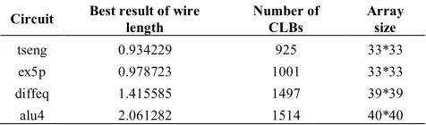
Using this table, we can say that this algorithm is more efficient in cases with smaller numbers of CLBs. The much larger size is of required FPGA; the more loses in algorithm reliability. Changes of both cost functions (wire length and overlap) for best results, the average and the worst results are summarized in Table 2; overlap field refers to the percentage of overlap occurrence in total circuit, and as mentioned, wire length is ratio of two considered cost functions. Fromthe data obtained in this study, it can be concluded that the Discrete-MOPSO algorithm has a more favorable result for smaller benchmarks, and for larger data, VPR would be more efficient method. Since only CLB blocks are inserted, more appropriate placement may be gained. PSO algorithm is one of the modern algorithm.The number of iterations is 50; this number has a direct relationship with the confidence factor of results. This means that, for example, in 10 iterations, data will have larger dispersion and the results will have no appropriate correlation, but with increasing the number of iterations, this dispersion is less tangible. This number is chosen in order to achieve stability in the results of the algorithm and remove bound of very high or very low answers. However, this parameter is not used as a variable in the problem definition. By increasing the number of repetitions, more reliable results can be obtained. With less than 20 iterations, distribution of results prevents us from correct analysis. Figures 1(a) and 1(b) depict the mentioned concept of Table 2 for the used benchmarks for wire length and overlap respectively:

TABLE 2. Range of answers for each benchmark

Circuit Best results Average results Worst results

Wire length overlap Wire length overlap Wire length overlap

tseng 0.934229 0.037668 0.974436 0.034115 1.001847 0.024048

ex5p 0.978723 0.080977 0.990932 0.074221 1.088682 0.070191

diffeq 1.125585 0.118276 1.273212 0.100417 1.531486 0.099552

(a) (b)

Figure 1. (a): Comparison of results for wire length, (b): comparison of results for wire length

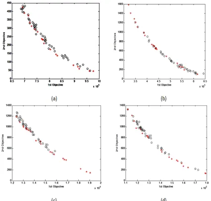
Figure 2. Two cost function of (a):"tseng", (b): "ex5p", (c):

diffeq", (d): “alu4

Using reasonable number of iterations, a good result can be obtained. Figure2 shows cost functions (wire length and overlap removal) of benchmarks. These figures consist of black circles and red stars; red stars are repository members. Final answer has been chose between the repository members. The spots in mentioned plots are considered as PSO particles in the last update and best results in one algorithm process. Asshown, only limited numbers of particles can be laid in repository. First objective is devoted to wire length cost function and is the calculation of wires of CLBs, so each of these figures may have different values of its objective. Times of overlap occurrence also are shown in the second objective. Minimum overlap case is selected between members in lowest level of vertical axis (overlap axis). Drawing of these figures is completely random, meaning that each time we repeat the algorithm, we get a new one. The art of using Discrete MOPSO algorithm is that to propel the results to decreasing two cost functions, and choose the best answer according to optimization benefits.Following figures are related to the mentioned benchmarks, the main idea for showing them is “Trade-off” issue in

optimization process. To consider both, the cost function the normalized wire length and overlap values are used. Normalized wire length actually is obtained by dividing the wire length of PSO to the results of using VPR. Also, overlap is divided by a specific coefficient according to simulation results. Figures 3 to 6, in the optimal overlap cases, draw overlap and its corresponding wire length in each of tested data. As seen, any increase in one of the cost functions, changes the other in a reduction process.

Figure 3. Trade off issue of “tseng”

Figure 4. Trade off issue of “ex5p”

Figure 6. Trade off issue of “alu4”

Like other evolutionary algorithms, PSO algorithm can lead to the conclusion of the convergence or divergence result. In addition,in basic equation, velocity is added to the position equation. This increase is controlled by limiting constraints of velocity (-Vmax , Vmax ). The Figure 2 shows both cost functions, and this fact can be realized that the concentrated points create a diagonal line, which results in the convergence of the algorithm. In case of divergence, the accumulation of particles and Pareto answers were not done on a regular pattern. On the other hand, discrete structure forced us to use some of Special functions to have applicable discrete algorithms. Based on programming codes, CLB blocks are placed only in certain places and the performance of the algorithm rises. Naturally CLB’s density in a particular location increase the overlap. But, this density causes reduction of wire length. However, minimizing overlap leads CLBs with more distance from each other, as a result, length of the wire increases.

5. FUTURE WORKS

Although this study sheds some light on FPGA placement by PSO, further research can be done on a number of issue. First: apply the Discrete-MOPSO algorithm to both CLB and IOB blocks with separate swarms. Second: apply the optimization algorithm to 3D data of FPGA placement. Third: more efficient compared with other optimization methods

6. CONCLUSION

In this paper, we introduced a Discrete multi-objective PSO (Discrete MOPSO) algorithm for placement stage in VLSI circuit design. It is known that placement is one of the most important and applicable issues in FPGA manufacturing process and reaching optimized results can be done by various procedures. Iteration methods and evolutionary principles got us to an algorithm that

optimized answer of designs by relocating the CLBs. The discrete nature of the CLBs forced us use DPSO. On the other hand, the two functions (wire length and overlap) need to be optimized simultaneously. So, we also took advantage of the MOPSO. In addition to being a multi-objective algorithm that is eventually reached, it was also used for discrete problems. The algorithm was tested on a number of standard benchmarks and compared to VPR, a known method in the field of FPGA placement. From the results we can say that the positive performance of the algorithm is increased by reducing the number of CLBs.Results of simultaneously surveys of cost functions, based on iterations and trade off issue of them also discussed.

7. REFERENCES

1. Kebbati, Y., "Modular approach for an asic integration of electrical drive controls", International Journal of

Engineering-Transactions B: Applications, Vol. 24, No. 2,

(2011), 107-115.

2. Xu, M., Gréwal, G. and Areibi, S., "Starplace: A new analytic method for fpga placement", Integration, the VLSI jouRnal, Vol. 44, No. 3, (2011), 192-204.

3. Shi, X., "Fpga placement methodologies: A survey", Dept. of

Computing Science, University of Alberta, (2009)1981-1986.

4. Xu, W., Xu, K. and Xu, X., "A novel placement algorithm for symmetrical fpga", in ASIC, 7th International Conference on, IEEE. (2007), 1281-1284.

5. Yang, M., Almaini, A., Wang, L. and Wang, P., "Fpga placement using genetic algorithm with simulated annealing", in ASIC, 6th International Conference On, IEEE. Vol. 2, (2005), 806-810.

6. Gudise, V.G. and Venayagamoorthy, G.K., "Fpga placement and routing using particle swarm optimization", in VLSI, 2004. Proceedings. IEEE Computer society Annual Symposium on, IEEE. (2004), 307-308.

7. Rout, P.K., Acharya, D. and Panda, G., "Novel pso based fpga placement techniques", in Computer and Communication Technology (ICCCT), International Conference on, IEEE. (2010), 630-634.

8. Peng, S.-j., Chen, G.-l. and Guo, W.-Z., "A discrete pso for partitioning in vlsi circuit", in Computational Intelligence and Software Engineering, CiSE. International Conference on, IEEE. (2009), 1-4.

9. El-Abd, M., Hassan, H. and Kamel, M.S., "Discrete and continuous particle swarm optimization for fpga placement", in Evolutionary Computation, CEC'09. IEEE Congress on, (2009), 706-711.

10. El-Abd, M., Hassan, H., Anis, M., Kamel, M.S. and Elmasry, M., "Discrete cooperative particle swarm optimization for fpga placement", Applied Soft Computing, Vol. 10, No. 1, (2010), 284-295.

11. Sarvi, M., Derakhshan, M. and Sedighizadeh, M., "A new intelligent controller for parallel DC/DC converters",

International Journal of Engineering-Transactions A: Basics,

Vol. 27, No. 1, (2013), 131-140.

13. Reddy, M.J. and Nagesh Kumar, D., "Multi‐objective particle swarm optimization for generating optimal trade‐offs in reservoir operation", Hydrological Processes, Vol. 21, No. 21, (2007), 2897-2909.

14. Premalatha, M.B., Divya, M.D., Abinaiya, M.N. and Monisha, M.S., "Particle swarm optimization based placement and routing of hardware tasks in 2d homogeneous FPGAS",International

Journal of Scientific & Engineering Research, Vol., 4, No. 3,

(2013), 1-6

.

15. Alvarez-Benitez, J.E., Everson, R.M. and Fieldsend, J.E., "A mopso algorithm based exclusively on pareto dominance concepts", in Evolutionary Multi-Criterion Optimization, Springer. (2005), 459-473.

16. MCNC benchmark suits, available: Http://www.Eecg.Toronto. Edu/~vaughn/vpr/vpr",

Discrete Multi Objective Particle Swarm Optimization Algorithm

for FPGA Placement

RESAECH NOTE

H. Akbarpour, G. Karimi, A. Sadeghzadeh

Department of Electrical Engineering, Faculty of Engineering, Razi University, Kermanshah, Iran

P A P E R I N F O

Paper history:

Received 10 April 2014

Received in revised form 26 October 2014 Accepted 13November 2014

Keywords:

Discrete MOPSO Optimization Algorithm FPGA Placement VLSI Design

Wire Length Cost Function Overlap Removal

ﺪﯿﮑﭼ ه

تاراﺪﻣﯽﮑﯾﺰﯿﻓﯽﺣاﺮﻃردﯽﺳﺎﺳاﻞﺣاﺮﻣزاﯽﮑﯾﯽﻫدﺎﺟ

VLSI

ﺖﺳا

.

لوژﺎﻣ،ﻪﻠﺣﺮﻣﻦﯾارد

لﻮﺻاﻖﺑﺎﻄﻣيراﺪﻣياﺰﺟاوﺎﻫ

نﺎﮑﻣرديزﺎﺳﻪﻨﯿﻬﺑ

ﯽﻣراﺮﻗﺺﺨﺸﻣيﺎﻫ

ﺪﻧﺮﯿﮔ

.

ﺪﻨﭼﺎﯾﮏﯾﺮﺑيراﺬﮔﺮﺛاويزﺎﺳﻪﻨﯿﻬﺑردﯽﻌﺳﯽﻫدﺎﺟﺪﻨﯾآﺮﻓﺮﻫ،ﻦﯾاﺮﺑﺎﻨﺑ

دراديزﺎﺳﻪﻨﯿﻬﺑرﻮﺘﮐﺎﻓ

.

ﯽﻣﯽﻓﺮﻃزا

ﻪﮐﺖﻔﮔناﻮﺗ

FPGA

يدﺮﺑرﺎﮐوﻦﯾﺮﺘﻤﻬﻣزاﮏﺷﯽﺑ،ﺎﻫ

زوريﺎﯿﻧدردﺎﻫراﺰﺑاﻦﯾﺮﺗ

ﺖﻗوفﺮﺻوﺪﻨﺘﺴﻫﮏﯿﻧوﺮﺘﮑﻟا

ﯾاﺮﺑ

يرﺎﺘﺧﺎﺳﯽﺳرﺮﺑويﺮﯿﮔدﺎﯿ

نﺎﺷ

ﺪﺷﺎﺒﯿﻣﯽﻣاﺰﻟا

.

ﺶﻧاد

VLSI

ﯽﯾﺎﻫرﺎﮑﻫارﻦﺘﻓﺎﯾلﺎﺒﻧدﻪﺑ

ﻪﻨﯾﺰﻫيزﺎﺳﻞﻗاﺪﺣﺖﻬﺟ

ﺎﺑﻂﺒﺗﺮﻣيﺎﻫ

FPGA

نآﺐﺳﺎﻨﻣدﺮﮑﻠﻤﻋﻦﯿﻤﻀﺗرﺎﻨﮐ ردﺎﻫ

ﺖﺳﺎﻫ

.

ﻢﺘﯾرﻮﮕﻟا

رديدﺪﻌﺘﻣيﺎﻫ

هزﻮﺣ

ردﯽﻫدﺎﺟي

FPGA

ﻪﺘﻓررﺎﮐﻪﺑﺎﻫ

ﺪﻧا

.

تارذهوﺮﮔﻢﺘﯾرﻮﮕﻟا

) PSO (

ﻢﺘﯾرﻮﮕﻟازاﯽﮑﯾ

ﻞﯿﺒﻗﻦﯾارديدﺮﺑرﺎﮐﯽﻠﻣﺎﮑﺗيﺎﻫ

ﻞﺋﺎﺴﻣ ﺖﺳا

.

ﻦﯾاﺮﺑﺎﻨﺑ ،

ﻢﯾدﺮﮐهدﺎﻔﺘﺳاﻪﻠﺌﺴﻣﻞﺣرد ﻢﺘﯾرﻮﮕﻟاﻦﯾازاﺎﻣ

.

،هژوﺮﭘﻦﯾارد

هﻮﯿﺷ

يزﺎﺳﻪﻨﯿﻬﺑﺖﻬﺟيﺪﯾﺪﺟي

ردﯽﻫدﺎﺟ

FPGA

ﺪﺷﻪﺋاراﺎﻫ

.

ﻦﯾوﺎﻨﻋﺎﺑفﺪﻫﻊﺑﺎﺗوديزﺎﺳﻪﻨﯿﻬﺑ،فﺪﻫ،ﺪﻨﯾآﺮﻓلﻮﻃرد

" ﻢﯿﺳلﻮﻃ " و " ﯽﻧﺎﺷﻮﭙﻤﻫ " ﯽﻣﻒﯾﺮﻌﺗ ددﺮﮔ . ﻪﺠﯿﺘﻧرد

ﻪﻓﺪﻫﺪﻨﭼﻢﺘﯾرﻮﮕﻟازاهدﺎﻔﺘﺳاﻪﺑرﻮﺒﺠﻣﺎﻣ

تارذهوﺮﮔي

) MOPSO ( ﻢﯾﺪﺷ . رﺎﺘﺧﺎﺳ MOPSO

ﻪﺘﺳد يارادﻪﮐﺖﺳايﻮﺤﻧ ﻪﺑ

باﻮﺟزايا

ﯽﻣﺎﻫ

ﺪﺷﺎﺑ

.

باﻮﺟﻪﺘﺳدﻦﯾاﻦﯿﺑزاﺎﻣو

ﻞﻗاﺪﺣﺎﺑباﻮﺟﮏﯾ،ﺖﺳرديﺎﻫ

ﻢﯾدﺮﮐﺶﻨﯾﺰﮔارﯽﻧﺎﺷﻮﭙﻤﻫ

.

ﻪﺘﺴﺴﮔﺖﯿﻫﺎﻣﻪﮐﺖﺳاﺮﮐذنﺎﯾﺎﺷ

يﺎﻫكﻮﻠﺑي

FPGA

يﻪﺨﺴﻧزاهدﺎﻔﺘﺳاﻪﺑرﻮﺒﺠﻣارﺎﻣ،

يﻪﺘﺴﺴﮔ

PSO

دﺮﮐ

.

زاﯽﺒﯿﮐﺮﺗﻪﺑزﺎﯿﻧﺎﻣ،ﻊﻗاورد

PSO

وﻪﻓﺪﻫﺪﻨﭼي

PSO

ﻢﯿﺘﺷادﻪﺘﺴﺴﮔي

.

ﺮﺑﻖﺒﻄﻨﻣﺖﺴﺗيﺎﻫهداد

MCNC benchmark

ﺪﻧا هﺪﺷ هدروآ ﺶﻫوﮋﭘ ﻦﯾا رد

.

هداد ﻦﯾا

ﯽﻫدﺎﺟ ﺖﺴﺗ لﻮﻤﻌﻣشور ﺎﺑ ﺎﻫ

) VPR ( ﻪﺴﯾﺎﻘﻣ ﺪﻧﺪﺷ .

ﯽﻣنﺎﺸﻧﺞﯾﺎﺘﻧ

د

ﺰﯾﺎﺳﺐﺳﺎﻨﻣبﺎﺨﺘﻧاﺎﺑﻪﮐﺪﻨﻫ

FPGA

، ﺦﺳﺎﭘ

دﻮﺑﺪﻫاﻮﺧلﻮﺼﺣﻞﺑﺎﻗﻪﻠﺌﺴﻣباﻮﺟياﺮﺑﯽﻘﻄﻨﻣيﺎﻫ

.