Numerical Simulation of the Wake Flow Behind an Ellipse using Random Vortex Method (RESEARCH NOTE)

(1)

RESEARCH NOTE

NUMERICAL SIMULATION OF THE WAKE FLOW BEHIND AN

ELLIPSE USING RANDOM VORTEX METHOD

G. Heidarinejad and S. Delfani

Department of Mechanical Engineering, Tarbiat Modarres University Tehran, Iran, [email protected]

(Received: May 12, 2002 – Accepted: February 6, 2003)

Abstract Direct numerical simulation of the wake flow around and behind a planar ellipse using a random vortex method is presented. Fluid is considered incompressible and the aspect ratios of ellipse and the angles of attacks are varied. This geometry can be a logical prelude to the more complex geometries, but less time dependent experimental measurements are available to validate the numerical results. Therefore, the key figures of the averaged values of selected cases are chosen to check the accuracy of the results. Based on the results, the general behavior of the flow around an ellipse at the zero angle of attack is almost similar to that around a circle. But, at the other angle of attacks, the asymmetry of the flow is dominant and pronounced clearly.

Key Words Random Vortex Method (RVM), Ellipse, Incompressible Viscous Flow

ﻩﺪﻴﻜﭼ

ﻱﺍﻪﺤﻔﺻﻲﻀﻴﺑﻚﻳﺖﺸﭘﺭﺩﻝﺎﻴﺳﻲﺘﺸﮔﺮﺑﻥﺎﻳﺮﺟﻲﻓﺩﺎﺼﺗﻪﺑﺍﺩﺮﮔﺵﻭﺭﺯﺍﻩﺩﺎﻔﺘﺳﺍﺎﺑﻪﻟﺎﻘﻣﻦﻳﺍﺭﺩ

ﺩﻮﺷﻲﻣﻪﺋﺍﺭﺍ

.

ﺴﻧﻭﻩﺪﺷﺽﺮﻓﺮﻳﺬﭘﺎﻧﻢﻛﺍﺮﺗﻝﺎﻴﺳ ﺪﻧﺍﻩﺪﺷﺽﺮﻓﺮﻴﻐﺘﻣﻪﻠﻤﺣﻪﻳﻭﺍﺯﻭﻲﻀﻴﺑﻱﺎﻫﺮﻄﻗﺖﺒ

.

ﻪﺳﺪﻨﻫ

ﺕﻻﺎﺣﻱﺍﺮﺑﻲﻛﺪﻧﺍﻲﻫﺎﮕﺸﻳﺎﻣﺯﺁﺞﻳﺎﺘﻧﻪﭼﺮﮔﺖﺳﺍﺮﺗﻩﺪﻴﭽﻴﭘﻱﺎﻫﻪﺳﺪﻨﻫﻱﺍﺮﺑﻲﺒﺳﺎﻨﻣﺭﺎﻴﺴﺑﺪﻣﺁﺭﺩﺶﻴﭘﻲﻀﻴﺑ

ﺮﺑﻲﻨﺘﺒﻣﻱﺪﻴﻠﻛﻱﺎﻬﺼﺧﺎﺷﺎﻣﺍﺪﻧﻮﺷﻪﺴﻳﺎﻘﻣﺎﻬﻧﺁﺎﺑﻪﻟﺎﻘﻣﻦﻳﺍﺯﺍﻞﺻﺎﺣﺞﻳﺎﺘﻧﺎﺗﺖﺳﺍﺖﺳﺩﺭﺩﻥﺎﻣﺯﻪﺑﻪﺘﺴﺑﺍﻭ

ﺮﻳﺩﺎﻘﻣ

ﺪﻧﺍ ﻩﺪﺷ ﻪﺴﻳﺎﻘﻣ ﺩﻮﺟﻮﻣﻲﻫﺎﮕﺸﻳﺎﻣﺯﺁ ﺮﻳﺩﺎﻘﻣﺎﺑ ﻭﺏﺎﺨﺘﻧﺍ ﺹﺎﺧ ﻱﺎﻫ ﺖﻟﺎﺣ ﻱﺍﺮﺑ ﻩﺪﺷﻱﺮﻴﮔ ﻂﺳﻮﺘﻣ

.

ﺎﺒﻳﺮﻘﺗ ﺮﻔﺻﻪﻠﻤﺣﻪﻳﻭﺍﺯ ﻱﺍﺮﺑ ﻲﻀﻴﺑﻑﺍﺮﻃﺍ ﻝﺎﻴﺳﻥﺎﻳﺮﺟ ﻲﻠﻛ ﺭﺎﺘﻓﺭ

" ﻲﻣﻲﻀﻴﺑ ﻚﻳﻑﺍﺮﻃﺍ ﺭﺩ ﻥﺁ ﺭﺎﺘﻓﺭﻪﻴﺒﺷ

ﺪﺷﺎﺑ

.

ﻼﻣﺎﻛﻭﺐﻟﺎﻏﻥﺎﻳﺮﺟﻥﺭﺎﻘﺗﻡﺪﻋ،ﻪﻠﻤﺣﻱﺎﻳﺍﻭﺯﺮﮕﻳﺩﺭﺩﺎﻣﺍ

"

ﺖﺳﺍﺱﻮﺴﺤﻣ

.

1. BACKGROUND

Unsteady viscous fluid flow; past two-dimensional bodies have been major areas of investigations by the computational fluid dynamics community. The flow past an elliptic cylinder involves the unsteady separation, high order vortex formation on the surface of the cylinder at moderate to high Reynolds numbers, and vortex-shedding phenomena for asymmetrically placed cylinders. Besides the Reynolds number, the angle of attack of uniform stream and ellipse eccentricity are parameters, which will influence the time dependent flow configuration.

Due to the fundamental and practical importance, this geometry has attracted a lot of efforts. One of the primary researches can be found in the work of Schilichting in 1968 [1]. In 1969, Schinel studied

(2)

numbers. Recently the mechanisms of flow past over an ellipse is studied by Mittal and Balachandar in 1996, Wang and Liu and Childress and Heidarinejad and Delfani in 1999 [9,10,11]. In this paper, the behavior of the instantaneous flow at a higher range of Reynolds number and a full range of angles of attack are presented. The results are classified into two main categories including the initial time and the long time after the flow is started. The averaged value of drag and lift coefficient, angle of separation and the different components of the velocity behind the selected cases are compared with the available experimental measurements.

2. GOVERNING EQUATIONS

The governing equations for an incompressible fluid in two dimensions are as follows:

0 . =

∇ u (1)

ω = ω ∇ + ∂ ω ∂

∇

2 Re 1 ..

t u (2)

Where:

y

u

x

v

∂

−

∂

=

ω

u

=0

on boundary

(3-1)

u

=

u

p

in time t=0

(3-2)

Definition of symbols is as following: u is the velocity vector with u and v as its components in x and y direction respectively, ω is the vorticity, up is the potential velocity at the initial times and Re is Reynolds number, Re=ρUL/µ, with U as the mean free stream velocity, L is the longer axe of ellipse. All variables are non-dimensionalized with respect to the proper scales.

Two mechanism are responsible for transport of vorticity namely convection and diffusion. In the random vortex method each time step is divided into two fractional steps. During each fractional step only one of the above-mentioned mechanisms

is considered as follows:

0

.

u

t

+

∇

ω

=

∂

ω

∂

(4) ω ∇ = ∂ ω ∂ 2 Re 1

t (5)

The velocity due to convection is related to the stream function ψ, which is the solution of Poisson's equation:

)

x

(

2

Ψ

=

−

ω

∇

(6) Where x v , y u ∂ Ψ ∂ = ∂ Ψ ∂ − =

Solution of Poisson's equation in an infinite domain, using the Green's function yields:

'

x

d

)

x

(

)

'

x

(

K

)

x

(

u

=

∫

−

ω

(7)

2 r ) x , y ( 2 1 ) ( K − π − = x And

dy

dx

'

x

d

=

3. NUMERICAL SCHEME

In random vortex method the vorticity field is discretized into a finite number of vortices known as vortex blobs. The induced vorticity and the resulting velocity, u_ω in an arbitrary point, x, would be:

)

'

x

(

f

)

x

(

_i N 1 i i

−

Γ

=

ω

_δ =

∑

(8)

) ( K ) ( _i N 1 i

i x x

x

u =

∑

Γ −

= δ

ω (9)

(3)

) r ( k r

) x , y ( 2

1 ) ( K

2 δ

− π −

= δ

δ x

And

2 i 2

i

2 ₍_x _x ₎ ₍_y _y ₎

r = − + −

Expressions for fδ and kδ known as core function

and Kernel are defined in accordance with Chorin [11,12,13]. Further details about the random vortex method and its convergence and stability are discussed in related references [14,15,16]. Transport of vorticity due to diffusion is in accordance with equation (5). In random vortex method the solution of this equation is the same as

adding a random walk, ηx and ηy, in both x and y direction respectively. These random walks are taken in accordance with a Gaussian statistical distribution with zero mean and standard deviation [17] equal to

Re t 2∆ = σ

Therefore the resulting total displacement in an infinite domain is:

xi i

i

i(t t) x (t) u (t)dt

x +∆ = +

∫

_ω +η (10-1)

∫

+η

+ = ∆

+ i _ωi yi

i(t t) y (t) v (t)dt

y (10-2)

(4)

Value of

∫

u_ω_i(t)dt and

∫

v_ω_i(t)dt are evaluated using a fourth order Runge-Kuta method.

4. BOUNDARY CONDITIONS

Boundary conditions of the governing equations require that the normal and tangential components of the total velocity are zero on the boundary of ellipse. Imaging method is used to make the normal component of velocity zero. In this paper, first the physical domain around ellipse, z, is mapped into a circle with radius R as the computational domain, ζ, using a conformal mapping ζ=ζ(z).

ζ + ζ

= c2

z (11)

And

16

) 1 AR ( ) 1 AR ( 2 c

2 2 ₌ + − +

In these relations AR is the aspect ratio of ellipse and c is the distance between its focuse. Later we use a modified version of a solver already developed by the same authors to solve for the flow around a circle [13].

Then for a vortex element in a distance r from the center of circle, two images are considered. The first image located in a distance R2/r with the opposite sign of the main vortex, and the other with the same sign but in the center of circle. In order to satisfy the no-slip condition on the solid wall, vortex sheets are employed. These vortices are initially generated on the solid boundary. Later due to the diffusion effects, they are separated from

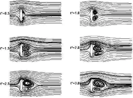
t*=0.5

t*=1.5

t*=2.5 t*=3.0

t*=2.0 t*=1.0

(5)

the solid wall and are moved inside the flow field. Within the distance ∆s from the solid wall, vortices are sheet type and beyond that they are considered blob type [13,18]. The induced velocity due to the vortex sheets at any arbitrary point, x, are calculated as follows:

∑

= ∆

− γ =

ω N

1 i

i if ( )

)

(x x x

S ) ( _w _i i

i

Γ = =

γ u

(12)

)} 2 S x ( H ) 2 S x ( H ){ y ( S 1

f_∆ = δ + − −

) ( K )

( _i

N

1 i

i x x

x

u =

∑

γ −

= ∆

(13) And

)} 2 S x ( H ) 2 S x ( H ){ y ( H ) (

K_∆ x = + − −

Definitions of variables are as following: δ(y) is Dirac delta function, H (x) is the Heavy side function, γi is the strength of sheet and S is the length of sheets respectively.

Once the velocities in the computational domain are calculated, they can be transformed into the physical plane using:

) ( dz d ) z

( = ζu ζ

u (14)

(6)

or cross the exit boundary downstream of the flow field are deleted.

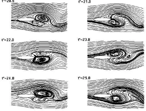
5. RESULTS AND DISCUSSIONS When the Reynolds number of the flow exceeds 40, the flow behind ellipse is divided into two regions, namely stable and unstable regions. The stable region forms during the initial times and, two almost symmetric eddies form next to the ellipse. The unstable region forms in the later times and also downstream of the flow field. Within this region the previously almost symmetric eddies become totally asymmetric, moving downstream, pairing and

forming an unstable region.

Stable Region

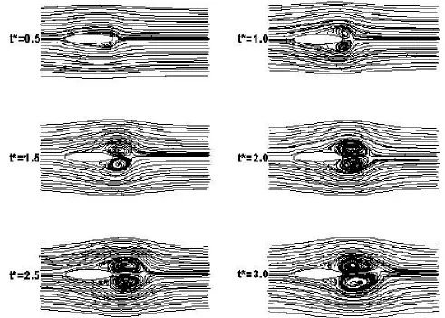
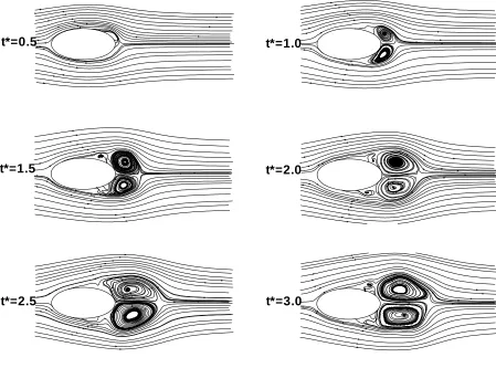
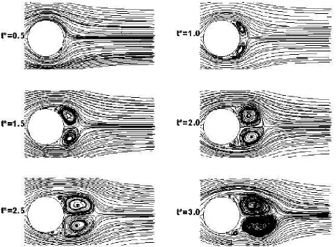
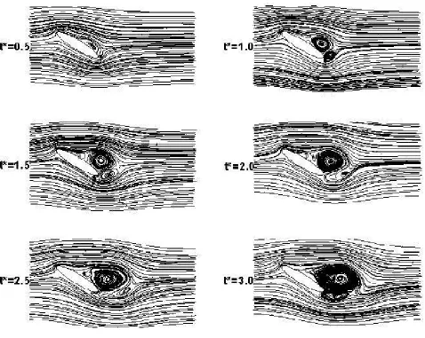
In order to capture some important aspects of the geometry of ellipse over a circle, we consider two important parameters: (a) aspect ratio and (b) the angle of attack. In Figure 1, 2, and 3 the streamlines around an ellipse during the initial times are plotted for different aspect ratios but with a zero angle of attack.

In Figure 1, 4 and 5 the streamlines around an ellipse during the initial times are plotted for different angle of attacks but for an aspect ratio of 0.2.

(7)

considered in two parts: next to ellipse and far downstream of it. First we focus on the areas next to ellipse. The instantaneous streamlines around the ellipse are plotted in Figure 6. Comparison of the flow structure in this figure with that in the Figures 1, 2 and 3 reveals the importance of time in formation of unstable zone and asymmetric structures.

There are not much available experimental measurements and numerical results around an ellipse to compare and validate our numerical results. Therefore, we focused on the special cases. In Figure 7, the instantaneous values of drag and lift coefficient, CD and CL, for an ellipse are plotted. The averaged value of CD and CL are in good agreement with the values listed in the related references [19].

In Figure 8 the averaged values of drag coefficient

for a wide range of Reynolds number for an ellipse with aspect ratio=1.0, a circle, are plotted and compared with the experimental measurements [20,21]. The numerical results show very good agreement with the experiment indicating the validity of the numerical scheme.

In Figure 9 the averaged values for the velocity on the symmetrical axis behind an ellipse with aspect ratio 1, a circle, are plotted and compared with the experimental measurements [20,21]. The results agree with the experiment and hence proving the accuracy of the results.

In Figure 10 the averaged values of separation angle versus time are plotted and compared with the experiment. The numerical results fall within the range of the experimental measurements [20,21].

(8)

Figure 6. Streamlines around ellipse at the later times with Re=3000, aspect ratio=0.2 and angle of attack=0 degrees.

(9)

downstream of the ellipse, and reveal the mechanisms of formation and paring of smaller eddies a long time run with a relatively longer computational domain is presented. In Figure 11 the velocity vector at the center of the computational elements, blobs are plotted.

By using an angle of attack=30 degrees, the instability of the flow is better pronounced. Clearly, the behavior of the flow is similar to that of a circle with almost the same Strouhal number [11,13]. Unfortunately, no experimental measurements were

available in this regard.

6. CONCLUSIONS

The numerical results show that the random vortex method can accurately simulate the turbulent flow around and downstream of an ellipse. Although there are not instantaneous experimental measurements available, but the results are in a good agreement with the little available data. The variation of the geometrical parameters has an important effect on the structure of flow. Among these parameters the effects of the angle of attack is more pronounced. There is a continuing research underway to use the results as a prelude to extend the scheme to more complex geometries.

7. REFERENCES

1. Schilichting, H., “Boundary Layer Theory”, McGraw-Hill, (1968).

2. Schindel, L., “Effects of Vortex Separation On Lift

Distribution of Elliptic Cylinders”, J. Aircraft, Vol. 6, No.

6, (1969), 537-543.

3. Lugt, H. J. and Haussling H. J., J. Fluid Mech., 65(4),

771, (1974), 771-782.

4. Daube, O. and Ta, P. L., “Etude Numerique D’ecoulements Instationnaires de Fluide Visqueux Incompressible Autour de Corps Profiles Par Une

Methode Combinee D’ordere O (h2) et O(h4)”, J. Mec,

Figure 8. The averaged values of: drag coefficient, D, versus Reynolds number, for an ellipse with Re=3000 and aspect ratio=1compared with experiment [20,21].

Figure 9. The averaged velocity on the symmetric axis behind an ellipse with Re=3000 and aspect ratio=1 compared with experiment [20,21].

(10)

Vol. 17, (1979), 651-678.

5. Giorgini, A. and Avci, C., “Impulsively Started Elliptic Cylinder at Re=3000: Catalog of two numerical

Experiments”, Technical Report CE-HSE-85-11,

Hydraulic and systems engineering, Purdue university, West Lafayette, Indiana, (1985).

6. Hamidi, A. and Giorgini, A., “Numerical Solution of the Navier Stokes Equations: Direct Radial Integration”,

technical report CE-HSE-85-02, hydraulic and systems

engineering, Purdue University, West Lafayette, Indiana, (1985).

7. Avci, C. and Giorgini, A., “High Order Vortex Formations

P as t E l l i p t i c C yl i n d er ”, A S C E I n t er d i vi s i o n a l

Conference, (1986), 24-44.

8. Blodgett, K. E. J., M. S. thesis, Department of Aerospace Engineering and Engineering Mechanics, University of Cincinnati, (unpublished), (1989).

9. Mittal, R. and Balachandar, S., “Direct Numerical

Simulation of Flow Past Elliptic Cylinders”, J. of Comput.

Physics 124, (1996), 351–367.

10. Wang, Z., Liu, J. and Childress, S., “Connection Between Corner Vortices and Shear Layer Instability in Flow Past

an Ellipse”, Physics of Fluids, Vol. 11, No. 9, (1999),

2446-2448.

11. Heidarinejad, G. and Delfani, S., “Simulation of Wake Flow Behind an Elliptical Cylinder at High Reynolds

Number by Random Vortex Method”, 6th Fluid Dynamic

Conference, Iran University of Science and Technology,

Tehran, Iran, (In Farsi), (1999), 199-210.

12. Chorin, A. J., “Numerical Simulation of Slightly Viscous

Flow”, J. Fluid Mech., Vol. 57, (1973), 785-796.

13. Heidarinejad, G. and Delfani, S., "Direct Numerical Simulation of the Wake Flow Behind a Cylinder Using Random Vortex Method in Medium to High Reynolds

Number", International Journal of Engineering, I.R.

Iran, Vol. 13, No. 3, (2000), 33-50.

14. Ghoniem, A. F. and Gagnon, Y., “Vortex Simulation of

Laminar Recirculating Flow”, J. Comput. Phys., Vol. 68,

(1987), 346-376.

15. Beal, J. T. and Majda, A., "Rates of Convergence for Viscous Splitting of the Navier Stokes Equation",

Mathematics Computation, Vol. 37, (1981), 209-243.

16. Beal, J. T. and Majda, A., "Vortex Methods II Higher Order Accuracy in Two and Three Dimensions",

Mathematics Computation, Vol. 39, (1982), 29-52.

17. Ghoniem, A. F. and Sherman, F. S., "Grid Free Simulation

of Diffusion Using Random Walk Methods", Journal of

Computational Physics, Vol. 61, No. 1, (1985), 1-37.