The Performance of an Hexahedron C* Element in Finite Element Analysis

International Journal of Engineering

J o u r n a l H o m e p a g e : w w w . i j e . i r

The Performance of an Hexahedron C

*

Element in Finite Element Analysis

G. H. Majzoobi*, B. Sharifi Hamadani

Department of Mechanical Engineering, University of Bu-Ali Sina, Hamedan, Iran

P A P E R I N F O

Paper history:

Received 26 November 2012 Received in revised form 02 March 2013 Accepted 18 April 2013

Keywords: Elasticity

Finite Element Method

*

C Elements Convergence

1

C Elements

A B S T R A C T

The performance of an 8-noded hexahedron C1* _{element in elasticity is investigated. Three translational} displacements and their derivatives as strain in each direction are considered as degrees of freedom (DOF) at each node. The geometric mapping is enforced using a C0 _{element with no derivative as} nodal DOF. The stiffness matrix of the element is also computed using a transformation matrix obtained from an equivalent C0 _{element. The results obtained from elastic stress analysis of a cantilever} show that: (i) the convergence rate of 8-noded C1* _{element is nearly equal to its equivalent C}0 _element, while it consumes less CPU time with respect to the C0 _{element; (ii) the element has successfully} passed the patch and distortion tests; (iii) the condition number of the stiffness matrix for C1* _{element is} less than the C0 _{element; (iv) the directly computation of strains as derivative DOF at the nodes along} with excellent convergence makes the C1* _{element superior compared with its equivalent C}0 _element.

doi:10.5829/idosi.ije.2013.26.10a.09

NOMENCLATURE

[k], {f} Stiffness matrix and force vector of _C0_element [K], {F} Stiffness matrix and force vector of _C*_element

* 1 C

N No. of DOF in a finite element mesh consisting of _C1* _{cubic elements}

0 C

N No. of DOF in a finite element mesh consisting of _C0 _{cubic elements}

z y

x n n

n , , No. of divisions in x,y and z directions

i

N¢ Geometric shape functions of super-parametric and sub-parametric element z

y

x, , Vectors containing the nodal coordinates and their derivatives with respect to global coordinates

*

i

N Shape functions of the 32-noded _Co _element

[ ]T Transformation matrix

[KLST] Stiffness matrix of linear strain triangular element

{ } {u = u v w} Vector containing the nodal DOF of _Co _element { } {U =U V W} Vector containing the nodal DOF of _C* _element { }ai Vector of unknown coefficients of field variable, a si, C Condition number

e Element distortion value

Greek Symbols

max

l Largest eigenvalue of the stiffness matrix

min

l Smallest eigenvalue of the stiffness matrix

*Corresponding Author Email: gh_majzoobi@yahoo.co.uk (G.H. Majzoobi)

1. INTRODUCTION

Finite element analysis is an approximate to the exact solution of differential equations. The rate of convergence to the exact solution has always been a concern. Basically, there are two types of convergence processes known as h-convergence and p-convergence methods in finite element method. In the first method, the order of the interpolating function remains constant and the number of elements increases progressively until some level of accuracy is reached. In the second approach, the mesh is fixed and the order of the interpolating function increases. Despite the disputes between researchers over the influence of orders of polynomials as interpolating function on the rate of convergence, numerical examples show that the rate of

p-convergence is substantially greater than h -convergence processes. The third scheme for evaluating the rate of convergence is called h-p convergence scheme which is a combination of h and p refinement. However, the practical implementation of the optimal h-p convergence processes is difficult and has been reviewed by some researchers [1, 2].

Since the appearance of finite element method, the attention of several researchers has been drawn to the inclusion of drilling freedom in plane elasticity finite element analysis. Drilling freedom is defined by rotation about the normal to the plane of element. Tocher and Hartz [3] examined this problem in 1967 but their element was computationally very inefficient. Further attempts by William [4], Youshida [5], Robinson [6], MacLeod [7] and some other researchers to solve the problem of inclusion of drilling freedom were all unsuccessful until 1984. At that time, Allman [8] could successfully include the drilling freedoms in the finite element method. His work was completed by Bergan and Fellipa [9, 10] in 1985 and Allman [11] in 1988. Cook [12] introduced a four-noded quadrilateral membrane element with two translational and one rotational degree of freedom at each node. Cook element improved by Macneal and Harder [13] turned into an element called QUADR which was then implemented in MSC/NASTRAN code and was found out to be a robust and accurate element.

Kelly and Kuruppu [14] proposed another convergence scheme called _C*_{convergence and}

suggested elements in which the nodal DOF included the derivatives of the displacement in each of the coordinate directions and introduced a family of elements for a _C*_{convergence algorithm to compete}

with h and p-convergence approaches. Bigdeli and Kelly [15- 17] reported the first two elements of such a family for two dimensional cases and established a new method called _C*_{convergence. They proved that the}

convergence of this family was better than h and p

-versions. They also realized that the best set of nodal DOF at the element level was the one consisting of freedom defined in element local coordinates( , )x h . This set would be transformed to the global coordinates (X, Y) at the assembly level by means of a transformation matrix [15]. Their elements significantly improved the accuracy of finite element results when solving problems with stress concentration and stress singularity.

In early family of elements developed in 1950’s for elasticity called _C0_{elements displacements, as DOF at}

their nodes, are forced to be continuous at nodes and in some cases along the boundaries. The derivatives of the displacements do not need to de continuous neither at the nodes nor along the boundaries. In 1960’s higher order elements such as _C1 _{elements appeared in which}

both displacements and their first derivatives are forced to be continuous at nodes or along the boundaries.

( 1)

r

C r³ elements known as Hermitian elements are widely used in the areas such as plate bending analysis.

r

C and _C*_{elements differ only on the continuity of the}

DOF. For _Cr_{elements, continuity is forced on the}

boundary while _C*_{elements enforce continuity only at}

the nodes. Moreover, in Hermitian finite element, displacements are defined to be transverse deflection and its derivatives to be the slope of that deflection. However, the family of _C*_{elements is designed for}

plane elasticity analysis with displacements defined to be in-plane deformations (i.e. u and v) and their derivatives to be nodal strains (i.e. ¶ ¶u x,

,

¶ ¶ ¶ ¶u y u z , ,¶ ¶v y, etc.).

In this work, a three dimensional 8-noded _C*

element is developed and its shape functions are derived. The convergence of the element is examined using patch and distortion tests. The ill-conditioning of the example is also investigated by computing the condition number of the stiffness matrix.

2. 2-D C*ELEMENTS FAMILY

The first element in the family of two dimensional _C*

elements is a 4-noded quadrilateral element shown in Figure 1(a). The element with only 2 DOF at each node is called _C0*_{element with the shape function defined as}

[15]:

(1 )(1 )/4 (i=1,2,3,4)

i i i

N = -x x -h h (1)

The second element called _C1*_{and shown in Figure 1(b)}

2 2 2

1 2 3 4 5 6 7

2 3 3 3 3

8 9 10 11 12

a a a a a a a

a a a a a

j x h xh h x h x

hx x h x h xh

= + + + + + +

+ + + + + (2)

The 12 constants of the equation are obtained using the 12 nodal DOF in each direction shown in Figure 1(b). The shape functions of this element were derived by Bigdeli can be found in reference [15].

A _C1* _{quadrilateral element with 12 DOF at each}

node is depicted in Figure 2. The field variable function of this element is expressed as follows in each direction [15]:

2 2 2 2

1 2 3 4 5 6 7 8

3 3 3 3 3 2 2 3

9 10 11 12 13 14

4 4 4 4 5 5

15 16 17 18 19 20

5 5 3 3 2 2

21 22 23 24

a a a a a a a a

a a a a a a

a a a a a a

a a a a

j x h xh h x h x hx

x h x h xh h x h x

x h x h xh h x

x h h x x h x h

= + + + + + + +

+ + + + + +

+ + + + + +

+ + + +

(3)

Figure 1. (a) A 4-noded quadrilateral C0element and (b) a 4-noded C1* element with 6 DOF at each node

Figure 2. A _C1* _{element with 12 DOF at each node}

3. 3-D C1*ELEMENTS FAMILY

In the present work, we have extended the 2 dimensional _C* _{elements to 3-D cases. The first}

member of _C*_{elements is the 8-noded hexahedron}

element with only three translational DOFat each node. The shape functions of this element can be found in the literature [18]. The second element of _C* _{family is C}1*

element. This element, as shown in Figure 3(a), has 12 DOF at each node. The field variable function of this element is expressed as follows:

2 2 2

1 2 3 4 5 6 7 8

3 3 3 2 2

9 10 11 12 11 12

2 2 2 2

13 14 15 16 17

3 3 3 3 3

18 19 20 21 22

3 2 2 2

23 22 23 24

3 3 3

25 26 27

+

a a a a a a a a

a a a a a a

a a a a a

a a a a a

a a a a

a a a

j x h h x z zx hz

xh h x z x z xh

hx h z z x hz xhz

h x x h zh hz x z

xz h xz x hz xhz

hx z xh z x hz

= + + + + + + +

+ + + + + +

+ + + +

+ + + + +

+ + + +

+ + + + 3

28

4 5 5 5

29 30 31 32

a

a a a a

xhz

xh h x x h

+ + + +

(4)

(a)

(b)

Figure 3. (a) A hexahedron 8-noded _C1*_{element (b) a} 32-noded _C0_element

Substituting the values of components of thevector

{

}

T

U = u v w and its derivatives, ui

x

¶

¶ , i

u

h

¶

¶ and i

u

V

¶

¶ (

, and

i

u =u v w ) at the 8 nodes of the element in Equations (4) and its derivatives, a system of 32 equations is produced, by solving which the 32 coefficients

a s

i, in field variable function are obtained. Using the coefficients, the shape functions of the element are obtained as follows:

( )( )( )( 2 2 2 )

1 1 1 1 2 /16

N= -_ëéx+ h- z+ x - +x h + +h z - -z ù_û (8-1)

( )( ) (2 )( )

2 1 1 1 1 /16

N = -é_ëx- x+ h- z+ ù_û (8-2)

( )( )( ) (2 )

3 1 1 1 1 /16

N =é_ëx+ h+ h- z+ ù_û (8-3)

( )( )( )2

4 1 1 1 /16

N _{= -}éx₊ h_- z₊ ù

ë û (8-4)

( )( )( )

(

2 2 2

)

5 1 1 1 2 /16

( )( ) (2 )( )

6 1 1 1 1 /16

N =é_ëx- x+ h+ z+ ù_{û (8-6)}

( )( )( ) (2 )

7 1 1 1 1 /16

N =é_ëx+ h- h+ z+ ù_{û (8-7)}

( )( )( )( )2

8 1 1 1 1 /16

N =é_ëx+ h+ z- z+ ù_{û (8-8)}

( )( )( )

(

2 2 2

)

9 1 1 1 2 /16

N =_ëéx- h+ z+ x + +x h - +h z - -z ù_û (8-9)

( )( ) (2 )( )

10 1 1 1 1 /16

N =é_ëx+ x- h+ z+ ù_û (8-10)

( )( )( ) (2 )

11 1 1 1 1 /16

N _{= -}éx_- h_- h₊ z₊ ù

ë û (8-11)

( )( )( )( )2

12 1 1 1 1 /16

N = -é_ëx- h+ z - z+ ù_û (8-12)

( )( )( )

(

2 2 2

)

13 1 1 1 2 /16

N = -_ëéx- h- z+ x + +x h + +h z - -z ù_û (8-13)

( )( ) (2 )( )

14 1 1 1 1 /16

N = -é_ëx+ x- h- z+ ù_û (8-14)

( )( )( ) (2 )

15 1 1 1 1 /16

N = -é_ëx- h+ h- z+ ù_û (8-15)

( )( )( )( )2

16 1 1 1 1 /16

N =é_ëx- h- z- z+ ù_û (8-16)

( )( )( )

(

2 2 2

)

17 1 1 1 2 /16

N = -_ëéx+ h- z- x - +x h + +h z + -z ù_û (8-17)

( )( ) (2 )( )

18 1 1 1 1 /16

N =é_ëx- x+ h- z- ù_û (8-18)

( )( )( ) (2 )

19 1 1 1 1 /16

N = -é_ëx+ h+ h- z- ù_û (8-19)

( )( )( )( )2

20 1 1 1 1 /16

N = -é_ëx+ h+ z+ z- ù_û (8-20)

( )( )( )

(

2 2 2

)

21 1 1 1 2 /16

N =_ëéx+ h+ z- x - +x h - +h z + -z ù_û (8-21)

( )( ) (2 )( )

22 1 1 1 1 /16

N = -é_ëx- x+ h+ z- ù_û (8-22)

( )( )( ) (2 )

23 1 1 1 1 /16

N _{= -}éx₊ h_- h₊ z_- ù

ë û (8-23)

( )( )( )( )2

24 1 1 1 1 /16

N =é_ëx+ h+ z+ z- ù_û (8-24)

( )( )( )

(

2 2 2

)

25 1 1 1 2 /16

N = -_ëéx- h+ z- x + +x h - +h z + -z ù_{û (8-25)}

( )( ) (2 )( )

26 1 1 1 1 /16

N = -é_ëx+ x- h+ z- ù_û (8-26)

( )( )( ) (2 )

27 1 1 1 1 /16

N =é_ëx- h- h+ z- ù_{û (8-27)}

( )( )( )( )2

28 1 1 1 1 /16

N = -é_ëx- h+ z+ z- ù_û (8-28)

( )( )( )

(

2 2 2

)

29 1 1 1 2 /16

N =_ëéx- h- z- x + +x h + +h z + -z ù_û (8-29)

( )( ) (2 )( )

30 1 1 1 1 /16

N =é_ëx+ x- h- z- ù_û (8-30)

( )( )( ) (2 )

31 1 1 1 1 /16

N =é_ëx- h+ h- z - ù_û (8-31)

( )( )( )( )2

32 1 1 1 1 /16

N =é_ëx- h- z+ z- ù_û (8-32)

Figure 4. An 8-noded _C2* _{element with 30 DOF at each node}

For the displacement in the three coordinate directions we can write:

32 32 32

1 1 1

, ,

i i i i i i

i i i

U N U V N V W N W

= = =

=

å

=

å

=

å

(9)

where the nodal DOF vector typically is given by:

{ } 1 1 1

1 1 1 1 1 1 1

... ... T T

i

U U U V V V W

U U V W

x h z x h x x

ì æ ö æ ö æ öæ ö æ ö æ ö æ ö¶ ¶ ¶ ¶ ¶ ¶ ¶ ü

ï ï

=í_ï ç ÷ ç ÷ ç ÷ç ÷ ç ÷ ç ÷ ç ÷_{è ø è ø è øè ø è ø è ø è ø¶ ¶ ¶ ¶ ¶ ¶ ¶} ý_ï

î þ (10)

If derivatives of Equation (10), U_, U_, U

x h z

¶ ¶ ¶

¶ ¶ ¶ ,

, , ,

V V V

h x z

¶ ¶ ¶

¶ ¶ ¶ , ,

W W W

x h z

¶ ¶ ¶

¶ ¶ ¶ are calculated at the

nodes, it will be seenthat the DOF are uniquely defined at the nodes. It can also be shown that the derivative DOF are not continuous along the boundaries of the element. The third element of _C* _{family is C}2*

element. Each nodes of this element has 30 DOF as shown in Figure 4. The field variable function of this element and its shape functions are too long and seem not to be practically useful for finite element analysis. Therefore, this work is confined only to the study of

1*

C element.

4. ADVANTAGE OF

C

*_ELEMENTS

The main feature of

C

*elements is that strains which are needed for stress calculations directly appear in the vector of nodal DOF. Definitely, strains are more accurately computed compared to the conventional relation

{ }

e =

[ ]

B U

{ }

, which requires difference operations on displacement components. The second feature of _C*_{elements which makes them more}

economical than their equivalent _C0 _{elements is the}

total DOF of the finite element model. Bigdeli [15] has shown that the following relation holds between the total number of equations for an 8-noded _C1* _{with 12}

DOF at each node (N_C1*) and a 32-noded

0

C

element with 3 DOF at each node (N_C0):

(

)

(

)

1*

0

12 12 12( ) 12

1

21 15 9( ) 3

x y z x y y z x z x y z

C

x y z x y y z x z x y z

C

n n n n n n n n n n n n

N

N n n n n n n n n n n n n

+ + + + + + +

= £

where

n

x, ny and

n

z are the number of divisions in x,

y and z directions, respectively. The above ratio becomes one for n_x=n_y=n_z =1 and approaches 0.57 for large

n

_x, n_y and

n

_z.

5. MAPPING IN 3-D C1*ELEMENTS

Elements are divided into 3 categories in finite element method. These are: iso-parametric, sub-parametric and super-parametric elements. Iso-parametric elements are those in which the shape functions for both the field variable and the geometry of the element are the same. For three dimensional iso-parametric elements we have:

1 1 1 1

, , , =

n n n n

i i i i i i i i

i i i i

x Nx y N y z Nz j Nj

= = = =

=

å

=

å

=

å

å

₍₁₂₎

All calculations in finite element methods are usually carried out in local coordinates,

x V

, and h. The transformation between derivatives of shape functions in global and local coordinates for three dimensional iso-parametric elements is performed using Jacobian matrix, [J], which is defined as follows:

[ ] T

T

i i i i i i

N N N N N N

J

x y z

x h V

¶ ¶ ¶ é¶ ¶ ¶ ù

é ù ₌

ê ú

ê_{¶ ¶ ¶} ú _{¶ ¶ ¶}

ë û ë û (13)

Equation (12) for super-parametric and sub-parametric elements is defined as follows:

( )

1 1 1

1

, , ,

= ,

n n n

i i i i i i

i i i

m

i i i i

i

x N x y N y z N z

N N N m n

j j

= = =

=

¢ ¢ ¢

= = =

¢ ¹ ¹

å

å

å

å

(14)

In order to extend the iso-parametric concept to the family of

C

* elements two methods are proposed; (1) using a 12, 20 or 32-noded

C

0 elements in which only translational DOF are prescribed and (2) using isoparametric geometry definition procedure (GDP). In the first method, the mapping of a hexahedron element from

xhV

coordinate system to xyz system is defined by the equation (15):

32 32 1 1 32 1 ( ) ( ) , ( ) ( ) , ( ) ( ) i i i i i i

x N x y N y

z N z

xhV xhV xhV xhV

xhV xhV = = = = = =

å

å

å

(15)

In which N_i is the shape function of the

C

1*element given by Equations (8-1) to (8-32) and x is the vector containing the nodal coordinates and their derivatives with respect to global coordinates. The vector is expressed as:

[

1 2 3 4 5 6 7 8

]

T T

x = x x x x x x x x (16)

T i i

i i i

x x x

x x

x h z

é æ¶ ö æ¶ ö æ¶ öù

= ê ç_¶ ÷ ç_¶ ÷ ç_¶ ÷ú

è ø è ø è ø

ë û (17)

The derivatives in Equation (17) are the components of a vector tangent to the node i and hence, they depend on the boundary geometry of the element which can be defined by

C

0_{elements of different orders as the}

boundary geometry doesn’t necessarily need to be expressed by

C

1*shape functions. Therefore, depending on the boundary geometry complexity, we can use 20-noded, 32-noded or even higher order

C

0elements for this purpose. For a 32-noded

C

0elements used in this work, we can write:

32 32 * * 1 1 32 * 1 ( ) ( ) , ( ) ( ) , ( ) ( )

i i i i

i i

i i

i

x N x y N y

z N z

xhV xhV xhV xhV

xhV xhV = = = = = =

å

å

å

(18)

where * i

N denotes the shape functions of the 32-noded 0

C element which can be found in the literature [18].

x

_i ,

y

_i and

z

_irepresent the global coordinates of the 32-noded _C0 _{element. By differentiating Equation (18),}

derivatives

i

x

x

æ¶ ö ç_¶ ÷ è ø

,

i

x

h

æ¶ ö ç_¶ ÷ è ø

, etc. can be calculated for the

four corner nodes of the _C1*_{element as follows:}

32 32 * * 1 1 32 * 1 ( ) ( ) , , ( ) , ...

i i i i i i i i i i

i i

i i

i i i i i i

i

N x N x

x x

N x

x

x h V x h V

x x h h

x h V

V V

= =

=

¶ ¶

æ¶ ö ₌ æ¶ ö ₌

ç_¶ ÷ _¶ ç_¶ ÷ _¶

è ø è ø

¶

æ¶ ö ₌

ç_¶ ÷ _¶

è ø

å å

å (19)

It must be mentioned again that 20-noded or even 8-noded _C0 _{element can be used to enforce the geometric}

mapping for _C1*_{element. In this work 32-noded C}0

element was employed for geometric mapping purpose. As will be explained in the next section, the derivatives in Equation (19) will be necessary for calculation of transformation matrix. In GDP method all necessary geometric data including geometric derivatives are extracted from the geometry definition of the problem using CAD packages at the modeling stage of the problem. This method has fully been described by Bigdeli [15] and is beyond the scope of this investigation.

6. TRANSFORMATION MATRIX

,

,

U U x U y U z

x y z

V V x V y V z

x y z

W W x W y W z

x y z

x x x x

x x x x

x x x x

¶ ₌¶ ¶ ₊¶ ¶ ₊¶ ¶ ¶ ¶ ¶ ¶ ¶ ¶ ¶ ¶ ₌¶ ¶ ₊¶ ¶ ₊¶ ¶ ¶ ¶ ¶ ¶ ¶ ¶ ¶ ¶ ₌¶ ¶ ₊¶ ¶ ₊¶ ¶ ¶ ¶ ¶ ¶ ¶ ¶ ¶ (20)

From Equation (20) and similar expressions for the other derivatives, the matrix form of the resultant equations is obtained at each node as:

12 1

1 0 0 0 0 0 0 0 0 0 0 0 0 1 0 0 0 0 0 0 0 0 0 0 0 0 1 0 0 0 0 0 0 0 0 0

0 0 0 0 0 0 0 0 0

0 0 0 0 0 0 0 0 0

.... .. .. ..

.. .. .. .. .. .. .. .. .. 0 0 0 0 0 0 0 0 0 U

V W

U x y z

V x y z

W x y z

x x x x

x x x x

V x x x

´

é ù é ù

ê ú ê ú

ê ú ê ú

ê ú ê ú

ê_¶ ú ê _{¶ ¶ ¶} ú

ê ú ê ú

ê¶ ú ê₌ ¶ ¶ ¶ ú

ê_¶ ú ê _{¶ ¶ ¶}

ê ú ê

ê¶ ú ê ¶ ¶ ¶

ê ú ê ê ú ê

ê_¶ ú ê _{¶ ¶ ¶}

ê_¶ ú ê _{¶ ¶ ¶}

ë û ë û

[ ]

12 1 12 1 12 12 .... .... U U V V W W U U

x _T x

V V x x W W z z ´ ´ ´

é ù é ù ê ú ê ú ê ú ê ú ê ú ê ú ê_¶ ú ê_¶ ú ê ú ê ú ê¶ ú₌ ê¶ ú úê ú_¶ ê_¶ ú úê ú ê ú ú ¶ê ú ê¶ ú úê ú ê ú úê ú ê ú ú ¶ê ú ê¶ ú úê ú_{ë¶ û} ê_ë¶ ú_û

(21)

For the 8-noded _C1*_{element the transformation}

matrix [T] will be a

[

96 96´

]

matrix. The geometric derivatives included in [T] can be calculated using Equation (19) as explained in section 5.

Another approach is to calculate the stiffness matrix of an element from the stiffness matrix of another element via a transformation matrix. This approach has been adapted by the authors such as Allman [8] and Cook [12]. Cook proved that the stiffness matrix [K] of the triangular element introduced by Allman [8] could be obtained from a linear strain triangle [KLST] with a

transformation matrix as [ ] [ ] [T ][ ]

LST

K =T K T . In his

further attempts, Cook obtained a 4-noded quadrilateral element from an 8-noded quadrilateral element which is known as Cook element. In this work, the DOF of a 32-noded _C0 _{hexahedron element with 3 DOF at each}

node are related to DOF of a _C1* _{8-noded hexahedron}

element with 12 DOF at each node (shown in Figure 4) to define a transformation matrix [T]. It is evident that both elements will have 96 DOF. The relation between the displacement vectors of the two elements is assumed to be of the form:

{ }

u =

[ ]{ }

T U (22)

where

{ }

u and

{ }

U are the nodal DOF of 0

C and _C*

elements, respectively. The finite element characteristic equation for the _C0_{element is assumed to be:}

[ ]

k u{ } { }= f (23)

Substituting Equation (22) in relation (23) yields:

[ ][ ]

k T U{ } { }= f (24)

If both sides of Equation (24) are multiplied by the transpose of the transformation matrix [T], we will obtain:

[ ] [ ][ ]

T T k T U{ }=

[ ]

T T{ }f Þ

[ ]

K U{ } { }= F (25) [K] and {F} are stiffness matrix and force vector of the new element which are defined as follows:

[ ] [ ] [ ][ ]

K = TT k T ,

{ }

F =

[ ] { }

TT f (26) In order to obtain the transformation matrix [T], we can employ the displacement function for the two elements, _C* _andC0_{. Let the displacement function for}

both elements is defined by Equation (4). For 32-noded

0

C hexahedron element, this equation can be rewritten as follows:

{ }u =[ ]{ }X a (27)

where {a} is the vector of the coefficients a s_i, in Equation (4) and {u} is the nodal displacement vector of

o

C element defined as:

{ } {

1 1 1 2 2 2 ... ...

}

T

u = u v w u v w (28)

Therefore, the vector of the coefficients a s_i, is obtained by solving a system of 32 linear equations. The matrix form of Equation (4) for 8-noded hexahedron _C*

element with 12 DOF at each node becomes:

{ }U =[ ]{ }B a (29)

where [B] is geometric matrix and {U} is the nodal displacement vector of

C

*element defined as:

{ } 1 1 1

1 1 1 1 1 1 1

... ... U U U V V V W U U V W

x h z x h x x

ì æ ö æ ö æ ö æ ö æ ö æ ö æ¶ ¶ ¶ ¶ ¶ ¶ ¶ ö ü

ï ï

=í ç ÷ ç ÷ ç ÷ ç ÷ ç ÷ ç ÷ ç_{¶ ¶ ¶ ¶ ¶ ¶ ¶} ÷ ý ï è ø è ø è ø è ø è ø è ø è ø ï

î þ (30)

Again, the vector of the coefficients ,a s_i is obtained by solving a system of 32 linear equations:

{ } [ ] { }1

a = B- U (31)

By substituting this equation in relation (27) we obtain:

{ }

[ ][ ]

1

{ }

u = X B- U (32)

From a comparison between Equations (32) and (22), the transformation matrix, [T], is obtained as follows:

[ ][ ]1

[ ]T = X B- (33)

be calculated. This approach was employed in the present investigation.

7. NUMERICAL RESULTS

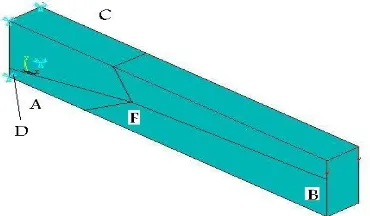
7. 1. Numerical Models The numerical simulation of a cantilever was used to study the performance of

1*

C elements with the mapping technique explained in section 5. The cantilever shown in Figure 5 is subjected to shear forces applied to the end of the beam as depicted in the figure. An elastic analysis with elasticity modulus,E=200GPa and Poisson's ratio, u=0.3 was used for the simulation.

In order to obtain a better understanding of the performance of _C1*_{elements, the results were compared}

with those obtained for 8-noded, 20-noded and 32-noded _C0_{hexahedron elements. The displacement of}

the end of the beam and the CPU time were measured from the simulations for each type of element.

7. 2. Numerical Results The results are illustrated in Figures 6 and 7 for displacement and CPU time, respectively. As the results shown in Figure 6 suggest, 8-noded_C1* _{and 32-noded C}0 _{elements converge more}

rapidly than the 20-noded and the 8-noded _C0_elements.

The convergence rate, however, is nearly the same for 8-noded_C1* _{and 32-noded C}0 _elements.

The variation of CPU time versus the number of elements is depicted in Figure 7. The figure clearly shows lower CPU time for 20-noded and 8-noded _C0

elements with respect to 8-noded _C1* _and

32-noded _C0 _{elements. This is obvious as the DOF of}

the two latter are less than those of the formers.

The interesting point is that the 8-noded_C1* _element

has consumed less CPU time than the 32-noded_C0_.

This is while both elements have the same number of

DOF. This confirms the advantages of

_C1*_elements

discussed in section 4. Moreover, 8-noded_C1* _elements

include first derivatives of displacement components are physical define the various components of the strain. Therefore, the use of 8-noded_C1*_{not only reduces the}

CPU time with respect to its equivalent _C0 _{element, but}

also saves the time for calculation of strains.

7. 3. Patch Test Patch test is a standard tool for assessing convergence of finite element for elasticity problems and was first introduced by Iron [20]. From the numerous publications on the theory and practice of the test which can be found in the literature [21-23] it can be deduced that the patch test is a necessary and

sufficient condition for assessing the convergence of any finite element approximation and has been accepted to be the most important check for practical finite element codes. Therefore, it is recommended to discard any element which fails to pass the test. The finite element model for patch test is shown in Figure 8.

Figure 5. The finite element model for a beam under bending

Figure 6. Variation of displacement versus number of elements for different element types

Figure 7. Variation of CPU time versus number of elements for different element types

0 1 2 3 4 5 6 7 8

0 10 20 30 40 50 60

Di

sp

lace

m

ent

(

mm)

No. of Elements

32-noded Element 4-noded C* element 8-Noded element 20-Noded element Theoritical value

0 100 200 300 400 500 600 700 800 900 1000

0 20 40 60 80 100

C

P

U

t

ime

(sec)

No. of elements

Figure 8. The finite element model for patch test

Figure 9. Variation of stress versus model number obtained from patch test

Figure 10. Variation of condition number versus number of elements

TABLE 1. The dimensions of various models used in patch test ( all units are in meters)

Model number A B C D F

1 0.3 1 1 0.3 (3,1)

2 0.1 1 1 0.7 (3,1)

3 7.5 1 1.5 0.1 (3,1)

4 0.5 1 1.5 0.2 (3,1)

5 9 1.5 0.5 0.2 (7,0.5)

6 9 1.5 0.5 0.1 (7,0.5)

7 3 0.7 0.1 1 (5,1)

The dimensions of various models which correspond to several extreme element geometries used in patch test are given in Table 1. As it is seen, there is no relation between the sizes of neighboring elements. The numerical results from the patch test are illustrated in Figure 9. The results clearly indicate that the element has passed the patch test successfully, as the stress has not shown sensitivity to variation in the finite element models used in the simulations.

7. 4. Condition Number Condition number is a numerical measure for evaluation of the solution sensitivity to the numerical drawbacks such as round-off error, mathematical operations, computational calculations and in general, ill-conditioning. The condition number is defined as C=lmax/lmin in which

max

l and l_min are the maximum and the minimum eigenvalues of the stiffness matrix [K]. A large value of

C can be a sign of ill-conditioning of the matrix. It can be shown [24] that for each power of ten in the ratio C=l_max/l_min the operations lose about one digit of accuracy in the displacement mode associated with

min

l . It is proved [15, 25, 26] that ill-conditioning and the growth of condition number with refinement in p -version number is worse than that of h-version. Bigdeli [15] has also shown that growth of condition number for

*

C convergence is better than p-convergence but remains worse than h-convergence.

In this work, the condition number has been obtained for the three dimensional 20 and 32-noded C0

and 8-noded _C1* _{elements. The numerical simulations}

carried out for the model are shown in Figure 5 as well as three other models with 4, 16 and 64 elements. The results are depicted in Figure 10. As the figure suggest, the condition number for 20 and 32-noded C0 elements rises to a maximum value at nearly 15 elements thereafter begins to decline and the number of elements used in this work (64 elements) for the main numerical simulations it nearly flats out. For 8-noded _C1*

elements, however, the variation of condition number versus number of elements is not as severe as observed for the other two elements. It is interesting to note that the condition number for 8-noded C1* element is significantly reduced at 64 elements.

7. 5. Distortion Test The test is used to investigate the effect of element distortion on the accuracy of a solution of a pure bending problem using different finite elements. This problem was first introduced by Zienkiewicz and Taylor [27] as higher order patch test and also suggested by Di and Ramm [28] for checking the accuracy of mixed and hybrid elements. In this test, a two elements beam subjected to a bending loading, as

0 100 200 300 400 500 600 700 800

0 2 4 6 8

Model No.

S

tr

es

s

(P

a)

0.00E+00 1.00E+09 2.00E+09 3.00E+09 4.00E+09 5.00E+09 6.00E+09 7.00E+09 8.00E+09 9.00E+09 1.00E+10

0 20 40 60 80

C

ond

it

ion

N

umb

er

No. of Elements

shown in Figure 11, is considered for demonstrating the distortion test.

The beam’s end deflection is obtained for different values of e as given in Table 2. The diagram of the error percentage of beam’s (with respect to the exact solution) end deflection versus e is illustrated in Figure 12. As it is observed, the highest error is obtained for 8-noded _C0

element but for the other three elements the situation is quite different. The 8-noded _C1* _{and 32-noded C}0

elements yield nearly the exact solution when there is no geometric distortion, e=0. For ef1, however, the

8-noded _C1*_{, 32-noded C}0 _{and 20-noded C}0 _elements

tend to become as rigid as 8-noded _C0 _{element. In}

general, 32-noded _C0 _{exhibits the best performance}

compared to other elements examined in this work.

Figure 11. The model used for distortion test

Figure 12. Variation of error percentage of the beam’s end deflection versus e

TABLE 2. Error percentage of the beam’s end deflection versus e

e=0 e=1 e=2 e=3 e=4

8-noded C0 71. 4 82.62 86.19 88.18 90.40

20-noded C0 2.96 6.069 19.29 48.90 70.77

32-noded C0 8.04 2.326 6.177 25.62 52.33

8-noded C1* 1.288 1.288 13.53 37.12 57.29

This is despite the fact that in all the tests described in previous sections, the 8-noded C1*element provides a better performance than the others. It is interesting to note that the trend of the results shown in Figure 9 is very similar to those given by Bigdeli [15] for 2-D _C*

elements.

8. CONCLUSIONS

From the numerical results, the following conclusions can be derived:

(1) The _C1*_{elements were studied here only for elastic}

analysis. It should be, however, checked for non-linear and dynamic analysis as well. This could be the subject of another research program.

(2) Mapping of _C1*_{elements (with extra DOF) can be}

forced by a transformation matrix.

(3) Transformation matrix can be obtained using equivalent_C0_{elements (with the same number of DOF).}

(4) The convergence rate of 8-noded_C1*_{element is}

nearly equal to its equivalent _C0 _{element, while it}

consumes less CPU time with respect to the _C0

element.

(5) The element has successfully passed the patch and distortion tests.

(6) The condition number of the stiffness matrix for_C1*

element is less than the _C0 _element.

The existence of derivative DOF at the nodes of _C1*

element along with the privileges mentioned above makes it superior compared to its equivalent _C0

element

Apart from the above conclusions, the new element should still be investigated from the point of view of its application in non-linear finite element contexts such as elasto-plastic and hyperelastic materials. Moreover, hourglassing is also a problem that if happens will dominate the solution and the results will become erroneous.

]

١

-٢٨

[

9. REFERENCES

1. Zhu, J. and Zienkiewicz, O., "Adaptive techniques in the finite element method", Communications in Applied Numerical

Methods, Vol. 4, No. 2, (1988), 197-204.

2. Zienkiewicz, O. C., Zhu, J. Z. and Gong, N. G., "Effective and practical h-p conversion adaptive analysis procedures for the finite element method", International Journal for Numerical

Methods in Engineering, Vol. 28, (1989), 879-891.

3. Tocher, J. L. and Hartz, B. J., "Higher order finite element for plane stress", J. Eng. Mech. Div. Proc. ASCE, Vol. 93, (1967), 149-172.

0 10 20 30 40 50 60 70 80 90 100

0 1 2 3 4 5

Err

o

r

p

er

ece

nt

age

e

4. William, K. J., Finite element analysis of cellular structures, in Department of Civil Engineering., University of California: Berkeley. (1969).

5. YOSHIDA, Y., "A hybrid stress element for thin shell analysis",

Finite Element Methods in Engineering, (1974), 271-284.

6. Robinson, J., "Four‐node quadrilateral stress membrane element with rotational stiffness", International Journal for Numerical

Methods in Engineering, Vol. 15, No. 10, (1980), 1567-1569.

7. Macleod, I. A., "New rectangular finite element for shear wall analysis", J. Struct. Div., ASCE, Vol. 95, No. 3, (1969), 399-409.

8. Allman, D., "A compatible triangular element including vertex rotations for plane elasticity analysis", Computers & Structures, Vol. 19, No. 1, (1984), 1-8.

9. Bergan, P. and Felippa, C., "A triangular membrane element with rotational degrees of freedom", Computer Methods in

Applied Mechanics and Engineering, Vol. 50, No. 1, (1985),

25-69.

10. Bergan, P. G. and Felippa, C. A., "“Efficient formulation of a triangular memberane element with drilling freedoms, infinite element methods for plate and shell structures, (eds) t.R. Hughes and e. Hinton, 1 (element technology)", pineridge Press International, (1986).

11. Allman, D., "Evaluation of the constant strain triangle with drilling rotations", International Journal for Numerical

Methods in Engineering, Vol. 26, No. 12, (1988), 2645-2655.

12. Cook, R. D., "On the allman triangle and a related quadrilateral element", Computers & Structures, Vol. 22, No. 6, (1986), 1065-1067.

13. Macneal, R. H. and Harder, R. L., "A refined four-noded membrane element with rotational degrees of freedom",

Computers & Structures, Vol. 28, No. 1, (1988), 75-84.

14. Kelly, D. W. and Kuruppu, M. D., Development of new four node plate and eight node hexahedron element with six nodal degrees of freedom, in Proceeding of the second Asian-pacific conference on computational mechanics.: Sydney, Australia, (1993). 145-149.

15. Bigdeli, B., An investigation of _C* _{convergence in the finite} element method, New South Wales University: Australia. (1996).

16. Bigdeli, B. and Kelly, D. W., _C* _{-convergence and nodal} derivatives in the finite element method, in First Australian

Congress on Applied Mechanics, The Institution on Engineers, Melbourne, Australia. (1996), 571-576.

17. Bigdeli, B. and Kelly, D. W., "_C* _{-convergence in the finite} element method", International Journal for Numerical

Methods in Engineering, Vol. 40, (1997), 4405-4425.

18. Stassa, F. L., "Applied finite element method", Cbs international editions, (1985).

19. Sharifi Hamadani, B., The study of the convergence of _C* elements in 3-d elasticity (in persian), in Mechnaical Enginnering Department., Bu-Ali Sina University: Hamadan, Iran,. (2001)

20. Irons, B. M. and Razzaque, A., "Experience with the patch test for convergence of finite element method, in mathematical foundation of the finite element method (eds) a.K. Aziz", Academic press, (1972).

21. Veubeke, D. and Fraeijs, B., "Variational principles and the patch test", International Journal for Numerical Methods in

Engineering, Vol. 8, No. 4, (1974), 783-801.

22. de Arantes e Oliveira, E., "The patch test and the general convergence criteria of the finite element method",

International Journal of Solids and Structures, Vol. 13, No. 3,

(1977), 159-178.

23. Razzaque, A., "The patch test for elements", International

Journal for Numerical Methods in Engineering, Vol. 22, No.

1, (1986), 63-71.

24. Rasanoff, R. A., Gloudeman, J. F. and Levy, S., Numerical conditioning of stiffness matrix formulations for frame structures, in Proceeding of the Second Conference on Matrix Method in Structural Mechanics., Wright-Patterson AFB: Ohio. (1968), 1029-1060.

25. Smith, B. F., Domain decomposition algorithms for the partial differential equations of linear elasticity, in Mathematics Department., New York University. (1991)

26. Babuška, I., Craig, A., Mandel, J. and Pitkäranta, J., "Efficient preconditioning for the p-version finite element method in two dimensions", SIAM Journal on Numerical Analysis, Vol. 28, No. 3, (1991), 624-661.

27. Dhatt, G. and Touzot, G., "Finite element method", John Wiley & Sons, (2012).

The Performance of an Hexahedron C

*

Element in Finite Element Analysis

G. H. Majzoobi, B. Sharifi Hamadani

Department of Mechanical Engineering, University of Bu-Ali Sina, Hamaden, Iran

P A P E R I N F O

Paper history:

Received 26 November 2012 Received in revised form 02 March 2013 Accepted 18 April 2013

Keywords: Elasticity

Finite Element Method

*

C Elements Convergence

1

C Elements

هﺪﯿﮑﭼ

عﻮﻧياهﺮﮔﺖﺸﻫﯽﺒﻌﮑﻣنﺎﻤﻟاﮏﯾدﺮﮑﻠﻤﻋ

C1*

ﺖﺳاهﺪﯾدﺮﮔﯽﺳرﺮﺑﻪﺘﯿﺴﯿﺘﺳﻻارد

.

نآتﺎﻘﺘﺸﻣوﯽﻟﺎﻘﺘﻧانﺎﮑﻣﺮﯿﯿﻐﺗﻪﺳ

ﺖﺳاهﺪﺷﻪﺘﻓﺮﮔﺮﻈﻧردهﺮﮔﺮﻫرديدازآتﺎﺟردناﻮﻨﻋﻪﺑﺖﻬﺟﺮﻫردﺶﻧﺮﮐناﻮﻨﻋﻪﺑﺎﻫ

.

زاهدﺎﻔﺘﺳاﺎﺑﯽﺳﺪﻨﻫﺖﺷﺎﮕﻧ

نﺎﻤﻟا

C0

ددﺮﮔﯽﻣلﺎﻤﻋادراﺪﻧياهﺮﮔيدازآتﺎﺟردناﻮﻨﻋﻪﺑﯽﻘﺘﺸﻣﭻﯿﻫﻪﮐ

.

زاهدﺎﻔﺘﺳاﺎﺑنﺎﻤﻟاﯽﺘﺨﺳﺲﯾﺮﺗﺎﻣﻦﯿﻨﭽﻤﻫ

نﺎﻤﻟازاﻪﮐﻞﯾﺪﺒﺗﺲﯾﺮﺗﺎﻣﮏﯾ

C0

ﺖﺳاهﺪﯾدﺮﮔﻪﺒﺳﺎﺤﻣﺪﯾآﯽﻣﺖﺳدﻪﺑنآلدﺎﻌﻣ

.

ﺶﻨﺗﻞﯿﻠﺤﺗزاهﺪﻣآﺖﺳدﻪﺑﺞﯾﺎﺘﻧ

ﻪﮐﺪﻫدﯽﻣنﺎﺸﻧرادﺮﯿﮔﺮﺳﮏﯾﺮﯿﺗﮏﯾ ﮏﯿﺘﺳﻻا

) : 1 (

عﻮﻧياهﺮﮔﺖﺸﻫنﺎﻤﻟاﯽﯾاﺮﮕﻤﻫخﺮﻧ

C1*

نﺎﻤﻟالدﺎﻌﻣًﺎﺒﯾﺮﻘﺗ

عﻮﻧلدﺎﻌﻣ

C0

نﺎﻤﻟاﻪﺑﺖﺒﺴﻧيﺮﺘﻤﮐشزادﺮﭘنﺎﻣزﻪﮐﯽﻟﺎﺣردﺖﺳانآ

C0

ددﺮﮔﯽﻣفﺮﺻ

) . 2 (

ﺖﯿﻘﻓﻮﻣرﻮﻃﻪﺑنﺎﻤﻟا

ﺖﺳاﻪﺘﺷاﺬﮔﺮﺳﺖﺸﭘارجﺎﺟﻮﻋاوﺮﯿﺴﻣيﺎﻫﺖﺴﺗﺰﯿﻣآ

) . 3 (

نﺎﻤﻟاﯽﺘﺨﺳﺲﯾﺮﺗﺎﻣﻪﺑطﻮﺑﺮﻣﺖﻟﺎﺣدﺪﻋ

C1*

زاﺮﺘﻤﮐ

نﺎﻤﻟا

C0

ﺖﺳا

. ) 4 (

ﯽﯾاﺮﮕﻤﻫﺎﺑهاﺮﻤﻫﺎﻫهﺮﮔيدازآتﺎﺟردتﺎﻘﺘﺸﻣناﻮﻨﻋﺖﺤﺗوﻢﯿﻘﺘﺴﻣرﻮﻃﻪﺑﺎﻫﺶﻧﺮﮐﻪﺒﺳﺎﺤﻣ

نﺎﻤﻟا،ﯽﻟﺎﻋ

C1*

نﺎﻤﻟاﺎﺑﻪﺴﯾﺎﻘﻣردار

C0

دزﺎﺳﯽﻣﺮﺗﺮﺑنآلدﺎﻌﻣ

.