InventoryControl.pdf

Inventory Control

9.1 ECONOMIC ORDER QUANTITY (EOQ)

The economic order quantity (EOQ) is the optimal quantity to order to replenish inventory, based on a off between inventory and ordering costs. The trade-off analysis assumes the following:

• Demand for items from inventory is continuous and at a constant rate. • Orders are placed to replenish inventory at regular intervals. • Ordering cost is fixed (independent of quantity ordered). • Replenishment is instantaneous.

Let

D = demand (number of items per unit time) A = ordering cost ($ per order)

c = cost of an item ($ per item)

r = inventory carrying charge (fraction per unit time) H = cr = holding cost of an item ($ per item per unit time) Q = order quantity (number of items per order)

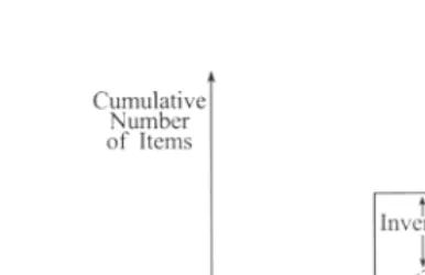
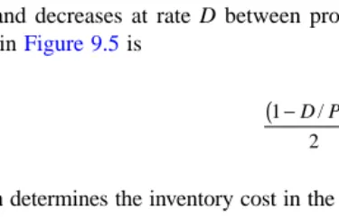
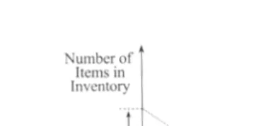
Figure 9.1 plots cumulative curves of orders and demand over time. The curve for orders increases in steps of size Q each time an order is placed, and the demand curve increases linearly with slope D. The height between these two curves at any point in time is the inventory level. Figure 9.2 plots this inventory level, which displays the classic sawtooth pattern over time. Inventory increases by Q each time an order is placed, and decreases at rate D between orders. The average inventory level in Figure 9.2 is Q/2, which determines the inventory cost in the EOQ model.

Total cost per unit time C(Q) is given by

(9.1)

The optimal quantity Q* to order (i.e., the order quantity that minimizes total cost) is given by

Hence

FIGURE 9.1 Cumulative orders and demand over time in EOQ model.

FIGURE 9.2 Inventory level over time in EOQ model.

C Q

HQ AD Q

( )

= +

Inventory Cost + Ordering Cost

2

d

(9.2)

Equation 9.2 for Q* is known as the EOQ formula. Figure 9.3 illustrates the trade-off between the inventory and ordering costs.

(Arrow, Karlin and Scarf, 1958; Cohen, 1985; Harris, 1913; Hax and Can-dea, 1984; Hopp and Spearman, 1996; Nahmias, 1989; Stevenson, 1986; Tersine, 1985; Wilson, 1934; Woolsey and Swanson, 1975).

9.2 ECONOMIC PRODUCTION QUANTITY (EPQ)

The economic production quantity (EPQ) is the optimal quantity to produce to replenish inventory, based on a trade-off between inventory and production set-up costs. The trade-off analysis assumes the following:

• Demand for items from inventory is continuous and at a constant rate. • Production runs to replenish inventory are made at regular intervals. • During a production run, the production of items is continuous and

at a constant rate.

• Production set-up cost is fixed (independent of quantity produced). The EPQ model is similar to that for the EOQ model. The difference is in the time to replenish inventory. The EOQ model assumes replenishment is instantaneous, while the EPQ model assumes replenishment is gradual, due to a finite production rate.

FIGURE 9.3 Trade-off between inventory and ordering costs in EOQ model.

Q AD

Let

D = demand (number of items per unit time)

P = production rate during a production run (number of items per unit time)

A = production set-up cost ($ per set-up) c = cost of an item ($ per item)

r = inventory carrying charge (fraction per unit time) H = cr = holding cost of an item ($ per item per unit time) Q = production quantity (number of items per production run)

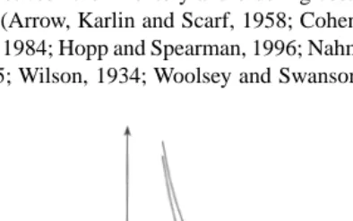
The EPQ model assumes P > D. Figure 9.4 plots cumulative curves of production and demand over time. The slope of the production curve during a production run is P. The slope of the demand curve is D. The height between these two curves at any point in time is the inventory level. Figure 9.5 plots this inventory level over time. Inventory increases at rate P – D during a production run, and decreases at rate D between production runs. The average inventory level in Figure 9.5 is

which determines the inventory cost in the EPQ model.

FIGURE 9.4 Cumulative production and demand over time in EPQ model. 1

Total cost per unit time C(Q) is given by

(9.3)

The optimal quantity Q* to produce (i.e., the production quantity that minimizes total cost) is given by

Hence

(9.4)

Equation 9.4 for Q* is known as the EPQ formula.

The trade-off between inventory and production set-up costs is the same as for the EOQ model illustrated in Figure 9.3, except for a different slope for the linear inventory cost curve. Note: as P approaches infinity, replenishment becomes instantaneous, and the EPQ formula given by Equation 9.4 reduces to the EOQ formula given by Equation 9.2.

(Hax and Candea, 1984; Hopp and Spearman, 1996; Nahmias, 1989; Steven-son, 1986; Taft, 1918; Tersine, 1985).

FIGURE 9.5 Inventory level over time in EPQ model.

C Q

H D P Q AD Q

( )

=

(

)

Inventory Cost + Production Set - Up Cost

1 2

/

d

dQC Q

( )

Q AD

H D P *

/ =

9.3 “NEWSBOY PROBLEM”: OPTIMAL INVENTORY TO

MEET UNCERTAIN DEMAND IN A SINGLE PERIOD

• cost of holding too many items and • cost of not meeting demand Let

c_o = cost per item of items left over after demand is met (overage cost per item)

c_s = cost per item of unmet demand (shortage cost per item) x = demand in given period (number of items)

f(x) = probability density function (pdf) of demand

F(x) = = cumulative distribution function of demand Q = quantity held in inventory (number of items)

The optimal cost trade-off depends on the expected numbers of items over demand and short of demand.

Expected cost C(Q) is given by

(9.5)

The optimal quantity Q* to hold in inventory (i.e., the quantity that mini-mizes expected cost) is given by

Applying Leibnitz’s rule for differentiation under the integral sign (see Section 13.8, Equation 13.23),

f u du x

( )

∫

0

C Q c E c E

c Q x f x dx C x Q f x dx s Q

s Q

( )

[

]

[

]

=

∫

(

) ( )

∫

(

) ( )

0 0

number of items over number of items short

d

Hence, setting C(Q) = 0, the optimal quantity Q* is given by

(9.6)

Equation 9.6 is the solution to the classic “Newsboy Problem.”

The overage and shortage costs, c_o and c_s, can be expressed in terms of the following economic parameters. Let

c = cost per item a = selling price per item p = lost sales penalty per item v = salvage value per item

The profit for each item sold is a – c. Hence, the lost profit per item for unmet demand is a – c. An additional cost of unmet demand is the lost sales penalty p, representing loss of some customers in future periods. Hence, the shortage cost cs is

cs = a – c + p

For unsold items left over after demand is met, the net cost per item is the cost minus the salvage value. Hence, the overage cost co is

co = c – v

d

dQC Q c Q Q x f x dx c Q x Q f x dx Q

s Q

( )

∫

{

(

) ( )

}

∫

{

(

) ( )

}

0 0

∂ ∂

∂ ∂

=c

∫

( )

∫

( )

s Q

0 0

=c F Q0

( )

{

( )

}

=

(

)

( )

d dQ

F Q c

c c s

s *

( )

From Equation 9.6, the optimal quantity Q* given by

(9.7)

(Hannsmann, 1962; Hopp and Spearman, 1996; Nahmias, 1989; Ravindran, Phil-lips, and Solberg, 1987).

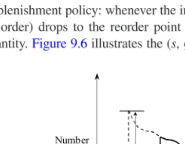
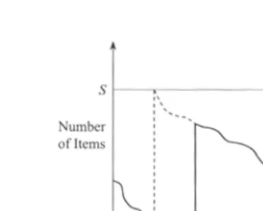
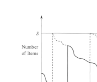
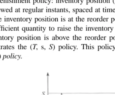
9.4 INVENTORY REPLENISHMENT POLICIES

Figures 9.6, 9.7, 9.8, and 9.9 illustrate the following basic policies for replenishing inventory in continuous review and periodic review systems:

• Continuous Review Systems

(s, Q) Policy: Whenever the inventory position (items on hand plus items on order) drops to a given level s or below, an order is placed for a fixed quantity Q.

(s, S) Policy: Whenever the inventory position (items on hand plus items on order) drops to a given level s or below, an order is placed for a sufficient quantity to bring the inventory position up to a given level S.

• Periodic Review Systems

(T, S) Policy: Inventory position (items on hand plus items on order) is reviewed at regular instants, spaced at time intervals of length T. At each review, an order is placed for a sufficient quantity to bring the inventory position up to a given level S.

(T, s, S) Policy: Inventory position (items on hand plus items on order) is reviewed at regular instants, spaced at time intervals of length T. At each review, if inventory position is at level s or below, an order is placed for a sufficient quantity to bring inven-tory position up to a given level S; if inventory position is above s, no order is placed. This policy is also known as a periodic review (s, S) policy.

(Elsayed and Boucher, 1985; Hadley and Whitin, 1963; Hax and Candea, 1984; Johnson and Montgomery, 1974; Silver, Pyke, and Peterson, 1998).

F Q a p c a p v *

The quantities Q, s, S, and T in these policies are defined as follows: Q = order quantity

s = reorder point S = order-up-to level

T = review period (time interval between reviews)

Notation for these quantities varies in the inventory literature. For example, some references denote the reorder point by R, while other references use R for the order-up-to level, and still others use R for the review period. The notation defined above is intended to avoid ambiguity, while being consistent with notation fre-quently used in the literature.

Inventory position is the sum of inventory on hand (i.e., items immediately available to meet demand) and inventory on order (i.e., items ordered but not yet arrived due to the lead time). The above policies for replenishment are based on inventory position, rather than simply inventory on hand, to account for cases where the lead time is longer than the time between replenishments. If the lead time is always shorter than the time between replenishments, then there will never be any items on order at the time an order is placed; in that case, the review of inventory can be based simply on the inventory on hand. (Evans et al., 1984; Johnson and Montgomery, 1974.)

A note on the continuous review systems: if demand occurs one item at a time, then the (s, S) policy is the same as the (s, Q) policy. If, however, demand can occur in batches, so that the inventory position can drop from a level above s to a level below s instantaneously (i.e., an overshoot can occur), then the (s, Q) and (s, S) policies are different. A comparison of Figures 9.6 and 9.7 illustrates the difference. In the (s, Q) policy, the order quantity is fixed, and the inventory position just after a replenishment order is placed is variable from one replen-ishment cycle to another. In the (s, S) policy, the inventory position just after a replenishment order is placed is fixed, and the order quantity is variable (Hax and Candea, 1984; Silver, Pyke and Peterson, 1998).

9.5 (

s

,

Q

) POLICY: ESTIMATES OF REORDER POINT (

s

)

AND ORDER QUANTITY (

Q

)

Replenishment policy: whenever the inventory position (items on hand plus items on order) drops to the reorder point s or below, an order is placed for a fixed quantity. Figure 9.6 illustrates the (s, Q) policy.

Assume:

• Demand for items is a random variable with fixed mean and variance. • Demands in separate increments of time are independent.

• Lead time (i.e., time from when an order for replenishment is placed until the replenishment arrives) is a random variable with fixed mean and variance.

• Lead times are independent.

Let

s = reorder point (number of items)

Q = order quantity (number of items)

D = average demand (number of items per unit time) σD2 = variance of demand (items2 per unit time)

L = average lead time (units of time) σL2 = variance of lead time (units of time2) FIGURE 9.6 Inventory pattern over time in (s, Q) policy.

2127_C09_frame Page 108 Friday, December 20, 2002 11:04 AM

k = service level factor A = ordering cost ($ per order)

H = holding cost of an item ($ per item per unit time)

The demand variance σD2is defined for demand in one time unit. Since the demands in each time unit are assumed to be independent, the variance of demand in a fixed time of t units is σD2t.

The reorder point s and order quantity Q in the (s, Q) policy are given approximately by

(9.8)

(9.9)

(Lewis, 1970; McClain and Thomas, 1985; Silver, Pyke and Peterson, 1998; Sipper and Bulfin, 1997; Stevenson, 1986).

In the special case of fixed lead times, σ_L2_{= 0 and Equation 9.8 for the}

reorder point s reduces to

(9.10) The order quantity Q, given by Equation 9.9, is the EOQ, as given in Section 9.1.

The reorder point s, given by Equation 9.8, is the inventory level needed to cover demand during the lead time. The first term, DL, is the inventory needed on average. The second term, , is the additional inventory needed to avoid stocking out due to random variability in demand and lead time. This additional inventory is the safety stock, i.e.,

(9.11) The above two terms for s are based on the result that demand during the lead time has mean DL and standard deviation (Hadley and Whitin, 1963).

s=DL+k LσDDσL

2 2 2

Q AD

H = 2

s=DL+kσD L

k LσD DσL

2 ₊ 2 2

Safety Stock = k LσD DσL

2 ₊ 2 2

LσD DσL

The service level factor k in Equations 9.8 and 9.11 is a dimensionless constant that represents the number of standard deviations beyond the mean DL needed to achieve a given service level (i.e., a given measure of performance for meeting demand from inventory). Service level is typically measured using one of the following two quantities, α and β:

α = probability of meeting demand from inventory

β = fraction of demand met from inventory (also known as “fill rate”) The probability α is the proportion of replenishment cycles in which no shortage occurs (regardless of the number of items short, when a shortage does occur). The fill rate β is the proportion of total items demanded that are filled from inventory (regardless of the number of replenishment cycles in which a shortage occurs).

If demand during the lead time has a general distribution with probability density function (pdf) denoted by f_l(x), then the quantities α and β are given by

(9.12)

and

(9.13)

where s is related to the service level factor k by Equation 9.8)

If demand during the lead time is normally distributed, then the quantities α and β are related to the service level factor k by

α = Φ(k) (9.14)

and

(9.15) α = −

( )

∞

∫

s

β = −1 1∞

∫

(

) ( )

β= −σ

π

(

)

[

( )

]

 

  

1 1

2 1

1 2

2

l

where Φ(k) is the cumulative distribution function of the standard normal distri-bution, i.e.,

(9.16)

and where σl is the standard deviation of demand during the lead time, i.e.,

(9.17)

(Fortuin, 1980; Nahmias, 1989; Schneider, 1981; Sipper and Bulfin, 1997). To ensure a high value of the probability α, the service level factor k is typically set in the range 2–3. From Equation 9.16, when k = 2, α = 97.7%, and when k = 3, α = 99.9% (Lewis, 1970; Mood, Graybill, and Boes, 1974; Sipper and Bulfin, 1997).

The relationship between the fill rate β and service level factor k is more complex than that for α, since it depends also on the order quantity Q. The EOQ given by Equation 9.9 provides a useful heuristic approximation for Q, which allows s to be estimated separately from Q. For given shortage cost per item, s and Q can also be optimized jointly (Hadley and Whitin, 1963; Nahmias, 1989; Sipper and Bulfin, 1997).

Note: if demand in each time unit is normally distributed and the lead time is constant (σ_L2_{= 0), then the demand during the lead time is normally distributed.}

If, however, demand in each time unit is normally distributed and the lead time is variable (σ_L2_{> 0), then, in general, the demand during the lead time is not}

normally distributed. In the case of variable lead time, therefore, the relationships between the safety level factor k and the quantities α and β, given by Equations 9.14 and 9.15, may not be sufficiently close approximations.

9.6 (

s

,

S

) POLICY: ESTIMATES OF REORDER POINT (

s

)

AND ORDER-UP-TO LEVEL (

S

)

Replenishment policy: whenever the inventory position (items on hand plus items on order) drops to the reorder point s or below, an order is placed for a sufficient quantity to raise the inventory position to the order-up-to level S. Figure 9.7

illustrates the (s, S) policy.

Φk x dx

k

( )

(

)

−∞

∫

1 2

1 2

2

π exp

σl= LσD+DσL

2 2 2

2127_C09_frame Page 111 Monday, December 23, 2002 7:11 AM

Assume:

• Demand for items is a random variable with fixed mean and variance. • Demands in separate increments of time are independent.

• Lead time (i.e., time from when an order for replenishment is placed until the replenishment arrives) is a random variable with fixed mean and variance.

• Lead times are independent. Let

s = reorder point (number of items) S = order-up-to level (number of items)

D = average demand (number of items per unit time) σD2 = variance of demand (items2 per unit time) L = average lead time (units of time) σL2 = variance of lead time (units of time2) k = service level factor

A = ordering cost ($ per order)

The demand variance σD2is defined for demand in one time unit. Since the demands in each time unit are assumed to be independent, the variance of demand in a fixed time of t units is σD2t.

The reorder point s and order-up-to level S in the (s, S) policy are given approximately by

(9.18)

S = s + Q (9.19)

where

(9.20)

(Hax and Candea, 1984; Silver, Pyke, and Peterson, 1998).

The reorder point s, given by Equation 9.18, is the inventory level needed to cover demand during the lead time. This expression for s is based on the result that demand during the lead time has mean DL and standard deviation

(Hadley and Whitin, 1963).

The service level factor k in Equation 9.18 is a dimensionless constant that represents the number of standard deviations demand beyond the mean DL needed to achieve a given service level (see the (s, Q) policy above).

The order-up-to level S, given by Equation 9.19, is a heuristic estimate based simply on the reorder point plus the EOQ, given in Section 9.1.

9.7 (

T

,

S

) POLICY: ESTIMATES OF REVIEW PERIOD (

T

)

AND ORDER-UP-TO LEVEL (

S

)

Replenishment policy: inventory position (items on hand plus items on order) is reviewed at regular instants, spaced at time intervals of length T. At each review, an order is placed for a sufficient quantity to raise the inventory position to the order-up-to level S. Figure 9.8 illustrates the (T, S) policy.

s=DL+k LσD+DσL

2 2 2

Q AD

H = 2

LσD DσL

Assume:

• Demand for items is a random variable with fixed mean and variance. • Demands in separate increments of time are independent.

• Lead time (i.e., time from when an order for replenishment is placed until the replenishment arrives) is a random variable with fixed mean and variance.

• Lead times are independent.

• Review period (i.e., time interval between reviews) is a constant. Let

T = review period (units of time) S = order-up-to level (number of items)

D = average demand (number of items per unit time) σD2 = variance of demand (items2 per unit time) L = average lead time (units of time) σL2 = variance of lead time (units of time2) k = service level factor

A = ordering cost ($ per order)

The ordering cost A in this policy includes the cost, if any, of reviewing the inventory position in each review period. The demand variance σ_D2_{is defined for}

demand in one time unit. Since the demands in each time unit are assumed to be independent, the variance of demand in a fixed time of t units is σ_D2_t.

The review period T and order-up-to level S in the (T, S) policy are given approximately by

(9.21)

(9.22) (Hax and Candea, 1984; Lewis, 1970; McClain and Thomas, 1985; Silver, Pyke, and Peterson, 1998; Sipper and Bulfin, 1997).

In the special case of fixed lead times, σL2= 0 and Equation 9.22 for the order-up-to level S reduces to

(9.23) The review period T, given by Equation 9.21, is determined from the EOQ, given in Section 9.1. For given EOQ denoted by Q, the optimal time between successive replenishments is Q/D. This provides the estimate for T. In practice, the review period T may be rounded to a whole number of days or weeks, or set at some other convenient interval of time.

The order-up-to level S, given by Equation 9.22, is the inventory needed to ensure a given service level (i.e., a given probability that demand is met). The first term, D(L + T), is the inventory needed to meet demand on average. The second term, , is the additional inventory (i.e., safety stock) needed to avoid stocking out due to random variability in the demand and the lead time.

Orders for replenishment in the (T, S) policy are placed every T time units, as shown in Figure 9.8. After an order is placed, it takes l time units for the replenishment to arrive, where l is a random variable (the lead time). Thus, the time from when an order for a replenishment is placed until the subsequent replenishment arrives (i.e., the time from ordering replenishment i to the arrival

T A

DH

= 2

S=D L

(

)

(

)

2 2 2

S=D L

(

)

(

)

k

(

)

of replenishment i + 1) is l + T. To avoid a shortage, therefore, the inventory in the (T, S) policy must be sufficient to meet demand during the lead time plus review period (rather than just the lead time, as in the (s, Q) policy). The demand during the lead time plus review period has mean D(L + T) and standard deviation

(Tijms and Groenevelt, 1984).

The service level factor k in Equation 9.22 is a dimensionless constant that represents the number of standard deviations beyond the mean needed to ensure a given service level (see (s, Q) policy).

9.8 (

T

,

s

,

S

) POLICY: ESTIMATES OF REVIEW PERIOD (

T

),

REORDER POINT (

s

), AND ORDER-UP-TO LEVEL (

S

)

FIGURE 9.9 Inventory pattern over time in (T, s, S) policy. k

(

)

Assume:

• Demand for items is a random variable with fixed mean and variance. • Demands in separate increments of time are independent.

• Lead time (i.e., time from when an order for replenishment is placed until the replenishment arrives) is a random variable with fixed mean and variance.

• Lead times are independent.

• Review period (i.e., time interval between reviews) is a constant. Let

T = review period (units of time) s = reorder point (number of items) S = order-up-to level (number of items)

D = average demand (number of items per unit time) σD2 = variance of demand (items2 per unit time) L = average lead time (units of time) σL2 = variance of lead time (units of time2) k = service level factor

A = ordering cost ($ per order)

H = holding cost of an item ($ per item per unit time)

The ordering cost A in this policy includes the cost, if any, of reviewing the inventory position in each review period. The demand variance σD2is defined for demand in one time unit. Since the demands in each time unit are assumed to be independent, the variance of demand in a fixed time of t units is σD2t.

Joint optimization of the three parameters (T, s, and S) in this policy leads to complicated mathematics (Lewis, 1970; Silver, Pyke, and Peterson, 1998). Simple heuristic approximations are presented here instead.

The review period T, reorder point s, and order-up-to level S in the (T, s, S) policy are given approximately by

(9.24)

T A

DH

(9.25)

S = s + Q (9.26)

where

(9.27)

(Porteus, 1985; Tijms and Groenevelt, 1984).

In the special case of fixed lead times, σL2= 0 and Equation 9.25 for the reorder point s reduces to

(9.28)

The review period T, given by Equation 9.24, is the same as for the (T, S) policy (i.e., it is obtained from T = Q/D). In practice, T may be rounded to a whole number of days or weeks, or set at some other convenient interval of time. The quantity Q, given by Equation 9.27, is the EOQ, given in Section 9.1.

The reorder point s, given by Equation 9.25, is the inventory level needed to cover demand during the lead time plus review period. This expression for s is based on the result that demand during the lead time plus review period has

mean D(L + T) and standard deviation .

The order-up-to level S, given by Equation 9.26, is the reorder point plus the EOQ, as in the (s, S) policy for a continuous review system.

The service level factor k in Equation 9.25 is a dimensionless constant that represents the number of standard deviations of lead time demand beyond the mean needed to achieve a given service level (see (s, Q) policy).

s=D L

(

)

(

)

2 2 2

Q AD

H = 2

s=D L

(

)

(

)

9.9 SUMMARY OF RESULTS FOR INVENTORY POLICIES

(Details given in preceding sections)

(s, Q) Policy:

(9.29)

(9.30)

(s, S) Policy:

(9.31)

S = s + Q (9.32)

(9.33)

(T, S) Policy:

(9.34)

(9.35)

(T, s, S) Policy:

(9.36)

(9.37)

S = s + Q (9.38)

(9.39) s=DL+k Lσ_D2+D2σ_L2

Q AD

H

= 2

s=DL+k Lσ_D2+D2σ_L2

Q AD

H

= 2

T A

DH

= 2

S=D L

(

)

(

)

T A

DH

= 2

s=D L

(

)

(

)

Q AD

H

= 2

2127_C09_frame Page 119 Monday, December 23, 2002 7:16 AM

9.10

INVENTORY IN A PRODUCTION/DISTRIBUTION

SYSTEM

The components of inventory in a production/distribution system are illustrated here for a single link between one origin and one destination.

Assume:

• Demand for items at the destination is continuous and at a constant rate. • The origin has a production cycle and makes production runs for the

destination at regular intervals.

• During a production run, the production of items at the origin for the destination is continuous and at a constant rate.

• The origin ships the items directly to the destination at regular intervals.

• The production schedule and shipment schedule are independent. • Transit time (i.e., time for a shipment to travel from the origin to the

destination) is a constant. Let

P = production rate at origin (number of items per unit time) D = demand at destination (number of items per unit time) Q = production lot size (number of items)

V = shipment size (number of items)

T = time interval between shipments (units of time) U = transit time (units of time)

I1 = inventory at origin due to production cycle schedule (number of

items)

I2 = inventory at origin due to shipment cycle schedule (number of

items)

I3 = in-transit inventory (number of items)

I₄ = inventory at destination due to shipment cycle schedule (number of items)

Let I1,

– I2,

– I3,

– and I4

–

denote the averages of I1, I2, I3, and I4 over time, respectively.

Figure 9.10 shows the cumulative production, shipments, and demand over time for the single link between one origin and one destination.

rate is P (where P > D to ensure demand is met). During the remainder of the production cycle, the production rate is zero. (The origin may produce items for other destinations during this time.)

The cumulative shipment departure curve in Figure 9.10 represents ship-ments from the origin. Each step in the curve represents a shipment of size V. The cumulative shipment arrival curve represents these shipments when they arrive at the destination, U time units later. The cumulative demand curve represents the demand at the destination, with rate D items per unit time.

The average slope of each cumulative curve in Figure 9.10 must be D to match the demand. The shipment size and the time between shipments are related by

V = DT (9.40)

The quantities I1, I2, I3, and I4 are the inventories at each stage in the

produc-tion/distribution system. At any point in time, the vertical distances between the cumulative curves in Figure 9.10 represent these inventories.

The average inventories I–₁, I–₂, I–₃, and I–₄ are given by

(9.41)

(9.42)

FIGURE 9.10 Cumulative production, shipments, and demand over time (Figure modified

from Blumenfeld et al., 1985, p. 370).

I Q D

P

1

2 1

= _ − _

I₂ V

2 = 2127_C09_frame Page 121 Friday, December 20, 2002 11:08 AM

(9.43)

(9.44)

(Blumenfeld et al., 1985; Hall, 1996).

Equation 9.41 for the average production cycle inventory I–₁ is the same as the expression for average inventory in the EPQ model, given in Section 9.2. The total number of items in inventory at the origin is the sum of two separate inventories: production cycle inventory I1 and shipment cycle inventory I2, as

shown in Figure 9.10.

Equations 9.42–9.44 for I2,

– I3,

– and I4

–

give the average components of the inventory associated with shipping. This inventory is, on average, made up of half a shipment at the origin, half a shipment at the destination, and DU items in transit. The total inventory associated with shipping is V + DU = D(T + U ) items.

9.11

A NOTE ON CUMULATIVE PLOTS

The cumulative plots of production, shipments, and demand over time (shown in Figure 9.10) provide a useful visual tool for representing the stages of a produc-tion/distribution system. A major benefit of cumulative plots is that they allow inventories at the various stages of the system to be conveniently displayed on one chart (Daganzo, 1991). For any point in time, the vertical distances between the cumulative curves represent the numbers of items in inventory at each stage, as indicated in Figure 9.10. If items pass through the system in a FIFO (first in, first out) sequence, the horizontal distances between the cumulative curves represent the times spent in inventory by an item at each stage.

Figures 9.1 and 9.4 show cumulative plots of orders and demand over time for the EOQ and EPQ models. For inventory systems in general, cumulative plots can be used to plan schedules for orders, analyze holding costs, and identify conditions for shortages (Brown, 1977; Daganzo, 1991; Love, 1979).

Cumulative plots also have applications in areas closely related to inventory control, such as queueing theory (Newell, 1982; Medhi, 1991) and transportation and traffic flow analysis (Daganzo, 1997; Newell, 1993). Cumulative plots have long been used in hydraulic engineering for determining reservoir capacity (Linsley and Franzini, 1955).

I3=DU