Volume 6, Issue 1 (2020)

1

THE RELATIONSHIP BETWEEN EXCHANGE RATES AND STOCK MARKETS

FOR THE FRAGILE FIVE COUNTRIES

Kadra Yusuf HERSI

Ayben KOY

Received: May 01, 2020 Accepted: May 26, 2020 Published: June 01, 2020

Abstract

This paper aims to determine the significance relation and direction of stock markets and exchange rate on Fragile five Countries (South Africa, Turkey, Indonesia, India, and Brazil) from January 2010 to December 2019. This study applied the VAR Analysis and Granger Causality Test to determine the relationship between exchange rates and stock indexes. The results show that South Africa and Turkey exchange rates and stock indexes are in bidirectional relationships, for India and Brazil, there is a one-way causality finding from the exchange rate to stock price, and the results for Indonesia show no causality.

Keywords:

Exchange Rate, Stock Indexes, Granger Causality.

JEL Code:

G10, G15

1.

Introduction

The "Fragile Five" is a term invented in 2013 by a Morgan Stanley financial analyst to characterize emerging market economies that were dependent on unreliable foreign investment to empower their development desires. This paper aims to determine the relationship for the stock markets and exchange rates on Fragile Five Countries (South Africa, Turkey, Indonesia, India, and Brazil) from January 2010 – December 2018. The period of the study was characterized to be a response to the global financial crisis recovery. Developed financial markets like the U.S. and the U.K., were improving from the financial crisis that happened in 2008. Many investors started moving their investment out of the emerging countries and back into U.S. dollars and Pounds. These powerful outflows originated principally from India, Brazil, Turkey, South Africa, and Indonesia. Their currencies—the Indian rupee, the Brazilian real, the Turkish lira, the South African rand, and finally the Indonesian rupiah. These currencies encountered significant vulnerability and made it difficult to finance their account deficits. Furthermore, this results in high co-movement between the exchange markets and the stock markets. Indeed, there has never been a period in which these two vital macroeconomic variables have moved so strongly.

2

2. Literature Review

There are two theoretical approaches background that propose the link between the stock market and the exchange market: a traditional approach and a portfolio approach. The traditional approach is about the "flow-oriented" exchange rate models (Dornbusch & Fischer 1980), recommending a Granger causality driving from exchange rates to stock prices, and it states that exchange rate fluctuations affect international competitiveness. Then the less favorable terms of trade may affect real income and so stock costs. Moreover, as a result of the estimated value of a stock equals the discounted add of its expected future capital flows, they react to macroeconomic events as well as the rate of exchange changes.

According to Evelyn (2010), the fluctuation in the exchange rate would influence the change in the firm's market value. Changes in market value will impact the investor's evaluation of the current and potential success of the company in the coming future, expressed in the strength of demand and supply in the company's stock exchange (Market Value). Consequently, the changes in demand and supply of stock shares would ultimately impact shifts in stock price. Local exchange depreciation would fuel export growth and rise in returns and drive its stock price up. At the same time, the company that imports more commodities in the depreciation of local the money would result in a rise in the cost of production impacting the company's earnings, which also affects the company's profits and its stock price (Yucel and Kurt, 2003).

According to Adler and Dumas (1984), the exchange rate also affects the companies which operate entirely in the domestic sphere. The impact lies in the input and output price changes of the company due to changes in macroeconomic conditions caused by exchange rate changes. However, the difference between the local currency exchange rate and foreign currencies will also influence the competitive position of the company against foreign competitors in the region.

Additionally, the portfolio approach is based on “stock- oriented” exchange rate forecasts, hence suggesting that the changes on exchange rates are because of the stock prices. The ‘stock-oriented’ model (Branson 1983; Frankel 1983) suggests that innovations in the stock market determine the capital of investors in demand for money. For instance, the rising stock price encourages capital inflows. It thereby increases the need for and thus appreciation of the local currency, which declares that if the domestic stock price rises, it will influence investors to buy more local goods by selling different products to obtain local currency. Expanded interest for the domestic money will lead to an appreciation of the domestic capital. On the other hand, an increase in the prices of local goods will increase wealth, which also will increase the demand for cash by investors. More foreign investment will be attracted by this situation, which will increase international demand for domestic currency, and the concluding result will be an appreciation of the local currency.

In sum, the theoretical structure implies that the causality of Granger may vary from exchange rates to stock prices or from stock prices to exchange rates. There is no conclusion on a theoretical aspect of the link between exchange rates and stock prices.

The outcomes of several studies find insufficient evidence of the relationship between exchange rates and stock prices (e.g Granger, Huang, and Yang, 2000; Smyth and Nandha, 2003; Hatemi-J and Roca, 2005; Patra and Poshakwale, 2006; Ehrmann Fratzscher and Rigobon, 2011; Chen and Chen, 2012), while others like (e.g., Tsagkanos & Siriopoulos (2013); Pan, Fok & Liu 2007; Jayasinghe & Tsui 2008; and Yau & Nieh 2009; Liang, Lin, and Hsu (2013)) discover that the relationship between exchange rates and stock prices is substantial and causal. Interestingly, research shows that granger causality is frequently divided into four catalogs of links on various financial markets: bidirectional relationships, unidirectional relationships between stock prices and exchange rates, unidirectional relationships between currencies, and stock prices, and no relationship.

Even though there is no agreement on either theoretical or empirical evidence on the relationship at a theoretical level between exchange rates and stock prices, in this sector we will examine both theoretically and empirically these two key lines of inquiry related to the interaction between stock prices and exchange rates.

3

exchange rates and noticed a clear negative correlation between stock prices and exchange rates. Besides, a dominant or deficient currency, rapid in the 1990s, can't change this outcome.

Donnelly and Sheey (1996), suggesting the causality path from exchange rates to stock prices, showed that the entire measure of UK stock market response to exchange rate fluctuations carries many months to operate into share prices.

Nieh & Lee (2001) analyzed the complicated relationship within exchange rates and stock prices for the G-7 countries (France, Germany, Canada, Italy, Japan, the United Kingdom, and the United States) applying regular data from 01/10/1993 until 15/02/1996. They find that short-term causality in Germany, Canada, and the UK, driving from exchange rates to stock prices, is particularly relevant for just a day. Explicitly, the German financial market will be excited by currency appreciation even though it reduces stock returns in Canada and the UK.

Abdalla & Murinde (1997) studied the changes in developing financial markets. Because of a lack of data availability, monthly data from India, Korea, the Islamic Republic of Pakistan, and also the Philippines from 01/1985 to 07/1994. He discovered that the relation linkage between exchange rates and stock prices reflects the traditional approach in India, Korea, and the Islamic Republic of Pakistan. It suggests the fluctuations in exchange rates confirm stock return changes in India, Korea, and the Islamic Republic of Pakistan.

As much as great empirical studies are supporting the traditional approach, there are the same amount of studies that show empirical proof for the portfolio approach, designating that there is unidirectional causality from stock prices to exchange rates. Ajayi and Mougoue (1996) suggested that a rise in the total domestic stock price has a negative short-run effect on local exchange value. In the long run, however, rises in stock prices have a positive impact on local exchange value. Ajayi et al. (1998), Investigating seven advanced markets and eight emerging Asian markets, it was found that equity markets and currency markets are interconnected with established markets, leading from stock returns to currency rates to causalities. Ramasamy and Yeung (2001) suggested that causality may vary depending on the study duration, and they also found that stock prices lead exchange rates for Malaysia, Singapore, Thailand, Taiwan, and Japan.

Also, the impact on the stock market can be substantial sufficient to make the real exchange rate appreciated as a consequence of expansionary monetary policy. To put in the away the stock market will significantly affect the foreign exchange rate market. Smith (1992) was in her early years, one of the proponents of the portfolio method. Smith (1992) uses quarterly data from the first quarter of 1974 to the third quarter of 1988 to research the correlation between exchange rates and stock prices in the United States. He used equities in the portfolio balance model of exchange rates to drive an approximate equation of exchange rates and found that stock prices in the UK would lead to adjustments in exchange rates between the UK pound and the US dollar. He technically reexamined this relationship, using a multi-country approach. Smith (1992b) revealed a theoretical model of optimal preference over risky assets to generate an approximate equation of the exchange rate. Unlike past examination, the assets involve equities, government bonds, and property. This model has been calculated using quarterly data from the 1974-1988 period. Everything was found that the German-U.S. mark value The dollar and the Japanese yen- US dollar exchange rates have a significant impact on their stock prices.

In many research for the developing markets, bidirectional causality between exchange rates and stock prices have been found. For reference, Granger, Huang & Yang (2000) used daily data from 03-0-1986 to 16-06-1998 to investigate the short-term dynamics between exchange rates and stock prices for several Asian countries during the Asian crisis. They conclude that there is a primary feedback relationship between the stock market and exchange rates in Hong Kong, Malaysia, Singapore, Thailand, and Taiwan. This result for Singapore and the Philippines is confirmed by Wongbangpo & Sharma (2002), based on monthly observations between 1985 and 1996.

The first study to propose this feedback interaction between the two markets was Bahmani-Oskooee and Sohrabian (1992). Cointegration and the Granger Causality tests are applied from 07-1973 to 12-1988, using monthly data. The findings imply a bidirectional correlation between exchange rates and US stock prices. Ajayi & Mougoue (1996) present similar results for France, Germany, Italy, Japan, the UK, and the US.

4

Some research suggests support relationships between the exchange rates and stock prices. For instance, Inci & Lee (2014) re-examines their complicated relationship between the two by integrating lagged effects and causal relationships, based on long-term annual data from 1984 to 2009. We point out that even this connection is vulnerable to the business circle. There Is compelling proof of bidirectional correlations among these two variables in France, Germany, Switzerland, the United Kingdom, the United States, Canada, and Japan. For India, Indonesia, and Korea, Lin (2012) confirms the result. Similarly, for the US, Canada, Japan, Italy, France, the UK, South Korea, and Hungary, Chen & Chen (2012) discover non-linear bidirectional relations between exchange rates and stock prices.

Moreover, there are particular theoretical structures for the collaboration between trade rates and stock costs, and there are a few investigations that cannot discover whatever connection between them in specific nations. It is just plain obvious, for instance, Granger, Huang, and Yang, 2000; Smyth and Nandha, 2003; Hatemi-J and Roca, 2005; Patra and Poshakwale, 2006; Ehrmann Fratzscher and Rigobon, 2011; Chen and Chen, 2012; among numerous others. For appearance, although Granger, Huang, and Yang (2000) find proof for the traditional and portfolio approach in individual nations, there is no indication of any connection between exchange rates and stock costs in Indonesia and Japan. A comparative outcome is found for Bangladesh and Pakistan by Smyth and Nandha (2003). Hatemi-J and Roca (2005) examined this adequate causality in the Asian emergency time frame.

The outcome shows that stock prices were not impacted by exchange rates, or lousy habit visa for Malaysia, Indonesia, the Philippines, and Thailand, during the Asian emergency. Around the same time, Mishra (2005) found that the Indian securities exchange wasn't identified with its foreign trade advertising, which is following the contentions of Hatemi-J and Roca (2005). Patra and Poshakwale (2006) analyzed the modifications of stock costs and they consider that the Athens stock trade is not recognized with its outside trade showcase, utilizing month to month information from 1990 to 1999 in their investigation. Ongoing examinations additionally affirm this sign. For instance, there is no proof of any momentary relations between trade rates and stock costs in the US, as proposed by Ehrmann Fratzscher and Rigobon (2011). Correspondingly, it is inconvenient. In summary, several studies have suggested no proof either of the conventional approach or the portfolio approach, implying that exchange rates and stock prices in the empirical literature may not be related to those countries.

3. Data and Methodology

We used a secondary data from weekly observations of the foreign exchange markets and stock markets. The data beginning from January 2010 to December 2019 includes the stock ‘index’ of Indonesia (JKII), South Africa (JTOPI), Turkey (XU100), Brazil (BVSP), and India (BSESN), and each countries’ currency against US Dollar. We used the Vector autoregression (VAR) model, Granger causality and impulse response tests of the VAR model. To apply the VAR model, the series should be stationary. In the first step, we used unit root tests. In the second step, VAR lag order selections are done for the stock index – exchange rate duals for each country. In the following steps, impulse response tests and Granger causality tests are done to examine the short term relationships for every dual.

3.1. Unit Root Test

Dickey-Fuller tests (DF test and ADF test)

One of probably the most famous and most commonly used unit root tests is the Dickey- test (Dickey, Fuller, 1979). It concentrated on the autoregressive first-order process model (Box, Jenkins,1970):

𝑦𝑡 = ∅1𝑦𝑡−1 +𝜀𝑡 t = 1,…, T (1)

where ∅1 is the autoregression parameter, 𝜀𝑡 is the non-systematic component of the model that meets the characteristics of the white noise process.

The null hypothesis is 𝐻0 = ∅1 = 1, i.e. the process contains a unit root and therefore it is non-stationary, and is denoted as I(1), alternative hypothesis is 𝐻1 : l ∅1 l < 1, i.e. the process does not contain a unit root and is stationary, I(0).

To calculate the test statistic for DF test, we use an equation that we get if 𝑦𝑡−1is subtracted from both sides of the equation (1):

5

𝑡𝐷𝐹= ∅1 −1

Sф₁ (3) where ∅1 is a least square estimate of ∅1 and Sф1 is its standard error estimate. Under the null hypothesis

this test statistic follows the Dickey-Fuller distribution, critical values for this distribution were obtained by a simulation and have been tabulated in Dickey (1976) and Fuller (1976).

3.2. Vector Autoregression Models (VAR) Analysis

VAR model is a blend of simultaneous equation methods and univariate time series models (Brooks 2008). VAR model is employed to get direct interdependencies among many time series. All variables used in the VAR model are viewed as endogenous, making it progressively adaptable to a more extensive cluster of factors (Brooks, 2008, p.6). The following are the purest form of the VAR model with only two equations as shown;

We may write the stationary, 𝑘-dimensional, VAR(p) process as

𝑦𝑡 = 𝐴1𝑦𝑡−1+ ⋯ + 𝐴𝑝𝑦𝑡−𝑝+ 𝐶𝑥𝑡 + 𝜀𝑡 (4)

Where

• 𝑦𝑡= (𝑦1𝑡,𝑦2𝑡,… . , 𝑦𝑘𝑡)′ is a vector of endogenous variables, • 𝑥𝑡= (𝑥1𝑡,𝑥2𝑡,… . , 𝑥𝑑𝑡)′ is a vector of exogenous variables, •𝐴1,… . , 𝐴𝑝 are 𝑘 × 𝑘 matrices of lag coefficients to be estimated, • 𝐶 is a 𝑘 × 𝑑 matrix of exogenous variable coefficients to be estimated,

• 𝜖𝑡= (𝜖1𝑡, 𝜖2𝑡, … 𝜖𝑘𝑡)′ is a 𝑘 × 1 white noise innovation process, with 𝐸(𝜖𝑡) = 0, 𝐸(𝜖𝑡𝜖𝑡’) = ∑ 𝜖 , and 𝐸(𝜖𝑡𝜖𝑠’) =0 for 𝑡 ≠ 𝑠 .

The last statement implies that the vector of innovations are contemporaneously correlated with full rank matrix ∑ 𝜖 , but are uncorrelated with their leads and lags of the innovations and (assuming the usual 𝑥𝑡 orthogonality) uncorrelated with all of the right-hand side variables.

3.3. Impulse Responses

The impulse response is an essential step in econometric studies that use autoregressive vector models. Their principal aim is to explain one or more evolution of the variables of a model in reaction to a shock. The above method allows tracking the transmission of a single shock within an equation structure that is otherwise noisy and therefore makes them very useful tools in the evaluation in time series.

3.4. Granger Causality

Granger Causality Analysis is a scientific test for determining if a single time series can predict the other. The resulting relationship can either be unidirectional or bidirectional (Hunter et al., 2017, p.3). Granger Causality test is usually used to investigate the short term connection among variables. It is precious to anticipate the progression of one variable with the assistance of another variable. One prerequisite for using the Granger causality test is establishing the stationarity of the variables.

Granger (1969) addresses the issue whether X triggers Y to see how much of the present Y can be clarified by Y's previous values, and then see if adding lagging X values will boost the interpretation. Y is said to be Granger-caused by X if X aids in predicting Y, or comparably if statistically important are the coefficients on the lagged X's. Note that two-way causation is repeatedly the case; 𝑋 Granger causes 𝑌 and 𝑌 Granger causes 𝑋.

It is significant to note that the declaration “𝑋 Granger causes 𝑌” does not imply that 𝑌 is the influence or the outcome of 𝑋. Granger causality measures superiority and information content but does not by itself indicate causality in the more common use of the term.

𝑦𝑡= 𝑎0+ 𝑎1𝑦𝑡−1+ ⋯ + 𝑎𝑙𝑦𝑡−1𝛽1𝑥𝑡−1+ ⋯ + 𝛽𝑙𝑥−1+ 𝜖𝑡 𝑥𝑡= 𝑎0+ 𝑎1𝑥𝑡−1+ ⋯ + 𝑎𝑙𝑥𝑡−1𝛽1𝑦𝑡−1+ ⋯ + 𝛽𝑙𝑦−1+ 𝑢𝑡

6

𝛽1= 𝛽2= ⋯ = 𝛽𝑙= 0 (6) Each equation. The null hypothesis is that in the last regression, X does not Granger-cause Y, and in the subsequent regression, X does not Granger-cause.

4. Empirical Results

When the stock index data by country are analyzed at the level value, H0 hypothesis is accepted since the prob>0.01 for all analyzed countries. When the first differences of the series were taken, H0 hypothesis is rejected as the prob<0.01 for all series.

4.1. UNIT ROOT TEST

Table 1. Unit Root Test For Stocks

Stocks

I(0) I(1)

Test Statistic Prob Test Statistic prob

Brazil -0.53029 0.8823 -8.49828 0.00*

India -0.29084 0.9235 -7.92183 0.00*

Indonesia -2.33993 0.1599 -5.98321 0.00*

South Africa -1.83556 0.3631 -6.0048 0.00*

Turkey -1.26648 0.6464 -7.07532 0.00*

*0.01, **0.05, ***0.10

When the exchange rate data by country are analyzed at the level value, H0 hypothesis is accepted as the prob>0.05 for all analyzed countries. When the first differences of the series were taken, H0 hypothesis was rejected because the prob<0.05 for all series. It is seen that exchange rate series become stable in the first difference.

Table 2. Unit Root Test Results for Exchange Rate Exchange

Rate

I(0) I(1)

Test Statistic Prob Test Statistic prob

Brazil -0.691986 0.8462 -5.458280 0.00

India -1.490961 0.5376 -5.944766 0.00

Indonesia -0.750504 0.8313 -9.960656 0.00

South Africa -1.121601 0.7087 -6.078535 0.00

Turkey 0.441096 0.9845 -6.542150 0.00

*0.01, **0.05, ***0.10

The lag length results for the variables discussed are shown in the next tables (Table 3-7). According to this table, it is seen that the lag length is 1 for the variables.

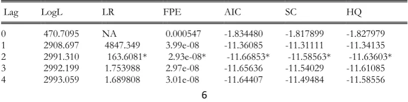
According to Table 3., the lag order for the model of India is taken to be two (2) as suggested by final prediction of LR, FPE, AIC, SC and finally HQ - Hannan-Quinn information criterion.

Table 3. VAR Lag Order for Indian Rupee and BSE SENSEX 30

Lag LogL LR FPE AIC SC HQ

0 470.7095 NA 0.000547 -1.834480 -1.817899 -1.827979

7

5 2994.525 2.869825 3.04e-08 -11.63415 -11.45176 -11.56265 6 2995.665 2.221799 3.07e-08 -11.62296 -11.40741 -11.53845 7 2996.146 0.933134 3.11e-08 -11.60918 -11.36047 -11.51168 8 2998.350 4.261860 3.14e-08 -11.60215 -11.32028 -11.49165

The lag order for the model Brazil is taken to be one (1) as suggested by final prediction of LR, FPE, AIC, SC and finally HQ - Hannan-Quinn information criterion (Table 4).

Table 4. VAR lag order for Brazilian Real and Bovespa

Lag LogL LR FPE AIC SC HQ

0 -71.30650 NA 0.004567 0.286914 0.303495 0.293414

1 2462.305 5037.474* 2.29e-07* -9.613719* -9.563976* -9.594218* 2 2463.171 1.714416 2.32e-07 -9.601451 -9.518548 -9.568950 3 2465.691 4.970518 2.33e-07 -9.595658 -9.479593 -9.550156 4 2468.134 4.800660 2.35e-07 -9.589565 -9.440339 -9.531064 5 2471.298 6.192769 2.35e-07 -9.586295 -9.403907 -9.514793 6 2472.700 2.731914 2.38e-07 -9.576125 -9.360576 -9.491623 7 2475.057 4.575085 2.39e-07 -9.569694 -9.320983 -9.472191 8 2476.891 3.545939 2.41e-07 -9.561216 -9.279344 -9.450713

The lag order for Turkey is chosen to be (5), as suggested by the concluding estimate of LR, FPE, AIC (Table 5).

Table 5. VAR lag order for Turkish Lira and BIST100

Lag LogL LR FPE AIC SC HQ

0 45.10938 NA 0.002896 -0.168726 -0.152145 -0.162225

1 2366.761 4616.043 3.33e-07 -9.239768 -9.190026* -9.220267*

2 2371.630 9.644045 3.32e-07 -9.243172 -9.160268 -9.210671

3 2375.449 7.533045 3.32e-07 -9.242463 -9.126398 -9.196961

4 2379.931 8.806476 3.31e-07 -9.244350 -9.095123 -9.185848

5 2387.752 15.30506* 3.26e-07* -9.259304* -9.076917 -9.187802

6 2389.940 4.265110 3.29e-07 -9.252213 -9.036664 -9.167711

7 2390.733 1.539420 3.33e-07 -9.239661 -8.990951 -9.142159

8 2392.675 3.753047 3.36e-07 -9.231603 -8.949731 -9.121100

Tabl e 4. Tabl e 4.

As shown in Table 6, for the model of South Africa, the lag order is taken to be one (1) as suggested by final prediction of LR, FPE, AIC, SC and HQ - Hannan-Quinn information criterion.

Table 6. VAR lag order for South African Rand and FTSE_JSE Top 40

Lag LogL LR FPE AIC SC HQ

0 436.1649 NA 0.000627 -1.699275 -1.682695 -1.692775

8

5 2534.079 7.840835 1.84e-07 -9.832013 -9.649625 -9.760511 6 2537.332 6.339466 1.85e-07 -9.829087 -9.613538 -9.744584 7 2539.275 3.773057 1.86e-07 -9.821038 -9.572328 -9.723535 8 2539.943 1.290377 1.89e-07 -9.807995 -9.526123 -9.697492

According to Table 7, the lag order for the model of Indonesia is taken to be five(5), as suggested by the final prediction of FPE and AIC.

Table 7. VAR lag order for Indonesian rupiah and Jakarta Islamic (JKII)

Lag LogL LR FPE AIC SC HQ

0 664.0365 NA 0.000257 -2.591141 -2.574560 -2.584641

1 2873.392 4392.770 4.58e-08 -11.22267 -11.17293 -11.20317 2 2887.682 28.30079 4.40e-08 -11.26294 -11.18004* -11.23044 3 2890.767 6.085380 4.42e-08 -11.25936 -11.14330 -11.21386 4 2906.899 31.69522 4.21e-08 -11.30685 -11.15762 -11.24834* 5 2912.692 11.33701 4.18e-08* -11.31386* -11.13148 -11.24236 6 2916.351 7.130540 4.19e-08 -11.31253 -11.09698 -11.22802 7 2918.765 4.686029 4.21e-08 -11.30632 -11.05761 -11.20882 8 2924.528 11.14423* 4.19e-08 -11.31322 -11.03135 -11.20272

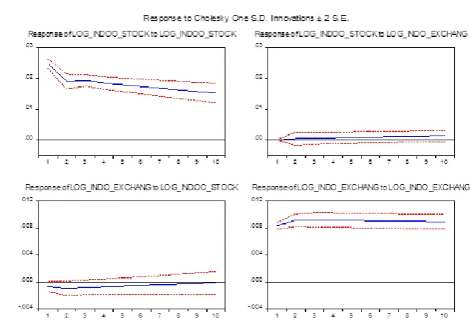
4.2. Impulse Response Tests

The impulse response function maps the effect of a one-time shock on one of the developments of the endogenous variables on current and future values. To examine the shock response on one variable to another; this analysis used Cholesky decomposition. Cholesky uses the inverse of the residual covariance matrix Cholesky factor to orthogonalize the impulses.

9

Figure 1: Impulse Response of Indian Rupee and BSE SENSEX 30

In the figure two, the responds of Bovespa and Brazilian Rupee to the shocks applied to each other are shown. According to the results, Brazilian Real responds to the shocks on Bovespa negatively but Bovespa does not responds to the shocks on Brazilian Real, which means no effect it around 0. Moreover, the negative respond of Bovespa does not decrease significantly in the first 10 weeks.

Figure 2: Impulse Response of Brazilian Real and Bovespa

10

Figure 3: Impulse Response of Turkish Lira and BIST100

South African Rand responds to the shocks on FTSE_JSE_40 positively. The positive respond in the first week increase thought out the 10th week. On the other hand, FTSE_JSE_40 responds to the shocks on South African Rand negatively. Stock index immediately fell, and it recover until the the 10th week.

Figure 4: Impulse Response of South African Rand and FTSE_JSE Top40

11

Figure 5: Impulse Response of Indonesian Rupiah and Jakarta Islamic (JKII)

4.3. Granger Causality Test

The causality test was applied to the series where the stationarity findings were obtained as a result of unit root tests. Analysis of the results shows the foreign exchange and stock prices for South Africa and Turkey are in a bidirectional relationship. For India and Brazil, there is a one-way causality finding from the exchange rate to the stock market indexes. Finally, any relation could not found between the stock market and the exchange market of Indonesia.

H0: There is no causality between the variables. H1: There is a causal relationship between the variables

Table 8. Granger Causality Test Results

Stocks → Exchange Rate Test Statistic df prob

Brazil 0.50857 2 0.7755

India 2.746441 2 0.2864

Indonesia 3.44909 2 0.4417

South Africa 9.442639 2 0.0089*

Turkey 5.128902 2 0.0770***

Exchange Rate → Stocks Test Statistic df prob

Brazil 5.028166 2 0.0809***

India 15.65251 2 0.0000*

Indonesia 2.305969 2 0.1127

South Africa 5.10141 2 0.0780***

Turkey 12.29221 2 0.0021*

*0.01, **0.05, ***0.10

5. Conclusion

12

tests, the causality relationship between stock markets and exchange rates varies on a country basis. While the bidirectional causality is found for South Africa and Turkey, a unidirectional causality from the exchange rate to the stock market is found for India and Brazil. Secondly, while the stock market index or exchange rate is not the Granger cause for each other, for Indonesia, weak reactions to shocks are seen by the help of impulse-response tests. The general results of the study show that the "flow-oriented" traditional approach is stronger, but we also found evidence on the "stock-oriented" approach on a country basis.

References

Abdalla, ISA and Murinde, V. 1997. Exchange rate and stock price interactions in emerging financial markets: evidence on India, Korea, Pakistan and the Philippines. Applied Financial Economics, 7: 25–35.

Aggarwal, R. (1981). Exchange rates and stock prices: a study of the United States capital markets under floating exchange rates. Akron Business and Economic Review, 21, 7-12.

Ajayi, R.A., Friedman, J. & Mehdian, S.M. (1998). On the relationship between stock returns and exchange rates: Test of Granger causality. Global Finance Journal, 9 (2), 241-251.

Alagidede, P., Panagiotidis, T., and Zhang, X. (2011) Causal relationship between stock prices and exchange rates, The Journal of International Trade & Economic Development, 20(1), pp. 67–86.

Bahami-Oskooee, M. & Sobrabian, A. (1992). Stock prices and the effective exchange rate of the dollar. Applied Economics, 24, 459-464.

Bala Ramasamy & Matthew C.H. Yeung, 2005. "The Causality Between Stock Returns And Exchange Rates: Revisited," Australian Economic Papers, Wiley Blackwell, vol. 44(2), pages 162-169.

Branson, W.H. (1983) Macroeconomic determinants of real exchange rate risk, In Managing foreign exchange rate risk, ed. R.J. Herring. Cambridge, MA: Cambridge University Press.

Chen, S.-W., and Chen, T.-C. (2012) Untangling the non-linear causal nexus between exchange rates and stock prices: New evidence from the OECD countries, Journal of Economic Studies, 39(2), pp. 231–259.

Doong, S., Yang, S. & Wang, A. T. (2005) The dynamic relationship and pricing of stocks and exchange rates: empirical evidence from Asian emerging markets, Journal of American Academy of Business, 7, pp118—123. Dornbusch, R. & S. Fischer, (1980). Exchange rates and current account. American Economic Review, 70,

960-971.Edwards, S. (2002). Contagion. The World Economy, 23 (7), 873-900.

Fang, W. and Miller, S. M. 2002. Currency depreciation and Korean stock market performance during the Asian financial crisis, University of Connecticut. Working Paper 2002–30

Granger, C. W.J., Huang, B.N. & Yang, C.W. (2000). A bivariate causality between stock prices and exchange rates:Evidence from recent Asian flu. The Quarterly Review of Economics and Finance, 40, 337-354.

Hatemi-J, and Roca, (2005) Exchange rates and stock prices interaction during good and bad times: Evidence from the ASEAN4 countries, Applied Financial Economics, 15, pp. 539–546.

Inci, A. C. & Lee, B. (2014) Dynamic relations between stock returns and exchange rate changes, European Financial Management, 20, pp71-106.

Liang, Lin, and Hsu (2013) Reexamining the relationships between stock prices and exchange rates in ASEAN-5 using panel Granger causality approach, Economic Modelling, 32, pp. 560–563.

Lin, (2012) The comovement between exchange rates and stock prices in the Asian emerging markets, International Review of Economics and Finance, 22(1), pp. 161–172.

Michael Adler and Bernard Dumas(1984), Financial Management Vol. 13, No. 2 pp. 41-50

Michael Ehrmann, Marcel Fratzscher, and Roberto Rigobon, "Stocks, Bonds, Money Markets and Exchange Rates: Measuring International Financial Transmission", Journal of Applied Econometrics, Vol. 26, No. 6, 2011, pp. 948-974.

Mishra, Alok Kumar, 2004. “Stock Market and Foreign Exchange Market in India: Are theyRelated?”, South Asian Journal of Management 11(2), pp. 12-31.

Murinde, V. & Poshakwale, S. (2004) Exchange rate and stock price interaction in the European emerging financial markets before and after Euro, unpublished paper presented at the 2004 EFMA Annual Meeting, Basel, Switzerland.

13

Pan, Fok, and Liu, (2007) Dynamic linkages between exchange rates and stock prices: Evidence from East Asian markets, International Review of Economics and Finance, 16, pp. 503–520.

Patra, T. & Poshakwale, S. (2006) Economic variables and stock market returns: evidence from the Athens stock exchange, Applied Financial Economics, 16, pp993–1005.

R. Smyth et al, Nandha(2003): Bivariate causality between exchange rates and stock prices in South Asia, Applied Economics Letters, Volume 10, 2003 - Issue 11

Ramasamy B. and Yeung M. (2001), Selective Capital Controls in Malaysia – Is it time to abandon them, Asia Pacific Finance Association Annual Conference, Bangkok, July 22 – 25 2001.

Raymond Donnelly and Edward Sheehy. “The Share Price Reaction of U.K. Exporters to Exchange Rate Movements: An Empirical Study” Journal of International Business Studies. Vol. 27, No. 1 (1st Qtr., 1996), pp. 157-165

Richard A. Ajayi, Mbodja Mougouė(1996) On the dynamic relation between stock prices and exchange rates: Journal of Financial Research, Vol.19, Issue2 1996 Pages 193-207

Smith, C. E. (1992b) Stock markets and the exchange rate: a multi-country approach, Journal of Macroeconomics, 14(4), pp697—629.

Soenen, L. A. & Hennigar, E. S. (1988) An analysis of exchange rates and stock prices--the U.S. experiences between 1980 and 1986, Akron Business and Economic Review, 19(4), pp7—16.

Stavarek, D. (2005) Stock prices and exchange rates in the EU and the USA: Evidence on their mutual interactions, Czech Journal of Economics and Finance, 55, pp141--161.

Tsagkanos, A. & Siriopoulos, C. (2013) A long-run relationship between stock price index and exchange rate: A structural nonparametric cointegrating regression approach, Journal of International Financial Markets, Institutions & Money, 25, pp106–118.

Wongbangpo, P. & Sharma, S. C. (2002) Stock market and macroeconomic fundamental dynamic interactions: ASEAN5 countries, Journal of Asian Economics, 13, pp27—51.

Wu, Ying, 2000. “Stock prices and exchange rates in a VEC model-the case of Singapore in the1990s”, Journal of Economics and Finance 24(3), pp. 260-274.