A computational method for key-performance-indicator-based parameter identification of industrial manipulators

R E S E A R C H

Open Access

A computational method for

key-performance-indicator-based parameter

identification of industrial manipulators

Felix Jost

_{, Manuel Kudruss}

_{, Stefan Körkel}

_{and Sebastian F Walter}

*_{Correspondence:}

[email protected] 2_{Interdisciplinary Center for} Scientific Computing, Heidelberg University, Im Neuenheimer Feld 205, 69120 Heidelberg, Germany Full list of author information is available at the end of the article

Abstract

We present a novel derivative-based parameter identification method to improve the precision at the tool center point of an industrial manipulator. The tool center point is directly considered in the optimization as part of the problem formulation as a key performance indicator. Additionally, our proposed method takes collision avoidance as special nonlinear constraints into account and is therefore suitable for industrial use. The performed numerical experiments show that the optimum experimental designs considering key performance indicators during optimization achieve a significant improvement in comparison to other methods. An improvement in terms of precision at the tool center point of 40% to 44% was achieved in experiments with three KUKA robots and 90 notional manipulator models compared to the heuristic experimental designs chosen by an experimenter as well as 10% to 19% compared to an existing state-of-the-art method.

Keywords: industrial manipulators; parameter identification; optimum experimental design; key performance indicator; quantity of interest; collision avoidance

1 Introduction

The total worldwide stock of operational industrial manipulators at the end of  is estimated between ,, and ,, units []. Of all the different industries, the automotive industry requires the largest share of nearly , manipulators []. One ap-plication area of manipulators in automotive industry are flexible measurement systems (FMS) in assembly lines. During measurements with FMS, industrial manipulators collect measurement data for quality and process control, e.g. of automotive bodies. This work-ing process requires a high tool center point (TCP) precision to detect production errors. The TCP defines the position and orientation of the working tool, which is attached to the last link of the manipulator.

1.1 Problem description

The TCP can be calculated using a geometric model of the manipulator by means of for-ward kinematics, e.g. the product of homogeneous transformations

W_{TCP(p,q) =} k

i= i–

i T(pi,qi) = k

i=

Ri(pi,qi) ci(pi,qi)

 

=

R(p,q) c(p,q)

 

, ()

wherei–_i T∈R×_{denotes the homogeneous transformation from the (i– )th to theith}

joint frame, where a frame is a Cartesian coordinate system attached to a joint. Each homo-geneous transformation can be represented by means of an orthogonal matrixRi∈SO() describing the orientation and a vectorc_i∈R _{describing the position of theith frame}

relative to the (i– )th frame. The pose of the TCP is given by the matrixR∈SO() de-scribing the orientation and the vectorc∈Rdescribing the position of the TCP in world coordinates, which is denoted by a  orW subscript if this is required for understanding.

The parametersp∈R·k_{describe the manipulator’s geometry such as the} • length of a link

• angle between two consecutive joint axes.

They are constant quantities, but due to manufacturing errors their exact values are un-known. In contrast,qi∈Ris a controllable value defining the pose of jointi. We denote by qeither a single configuration of the manipulator, i.e.q∈Rk_{, or a set ofnconfigurations,}

i.e.q∈Rn·k_{, depending on the context. The homogeneous transformations}i–

i T, defining

the position and orientation of linkiwith respect to link (i– ), can be described in the

Denavit-Hartenbergconvention []

i–

i TDH(pi,qi) = TRz(pi,+qi)TTz(pi,)TTx(pi,)TRx(pi,),

where

TRz(θi) = ⎡ ⎢ ⎢ ⎢ ⎣

cos(θi) –sin(θi)   sin(θi) cos(θi)  

        ⎤ ⎥ ⎥ ⎥

⎦, TTz(di) = ⎡ ⎢ ⎢ ⎢ ⎣  I,  di   ⎤ ⎥ ⎥ ⎥ ⎦,

TRx(αi) = ⎡ ⎢ ⎢ ⎢ ⎣    

 cos(αi) –sin(αi) 

 sin(αi) cos(αi) 

   

⎤ ⎥ ⎥ ⎥

⎦, TTx(ai) = ⎡ ⎢ ⎢ ⎢ ⎣ ai I,     ⎤ ⎥ ⎥ ⎥ ⎦.

T∈R_{represents again a homogeneous transformation with the subscriptsR,T}

speci-fying the type, i.e. rotation or translation, and the additional subscriptsx,y,zdenote the respective coordinate axis along or around the transformation takes place. Alternatively, theHayaticonvention [] can be used in the case two consecutive joints are parallel or almost parallel. Please note that the methodology derived in this article is not dependent on the chosen kinematic representation.

.. Parameter identification of industrial manipulators

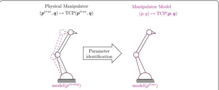
The idea of parameter identification of manipulators is visualized in Figure . Parame-ter identification of manipulators and of more general industrial mechanisms, e.g. gantry manipulators orGough-Stewartplatforms, is required whenever differences between the model representing theidealmanipulator, e.g. (), and the real manipulator exist. These differences are due to a mismatch between the parameterspof the model and the true parametersptrue_{of the real manipulator causing a systematic error}

Figure 1 Concept of parameter identification of industrial manipulators.Unknown geometric parametersplead to deviations between model prediction and actual tool center point (TCP) pose. On the left, the actual TCP poseTCP(ptrue_{,q) (in solid-black) and the predicted TCP poseTCP(p,q) (in red-dashed)}

are shown before the parameter identification and they do not coincide. The identification tries to eliminate these deviations by estimating the true parameters of the real manipulator. On the right, the actual TCP pose (in solid-black) and the predicted TCP pose (in red-dashed) coincide after the parameter identification procedure (forp=ptrue_).

between model-predicted and real TCP. Such deviations occur due to manufacturing tol-erances, material failure, different environmental conditions like temperature and other effects. This mismatch can be reduced by exact identification of the mathematical model of the industrial manipulator, i.e. by adjusting the mathematical model to the real manip-ulator geometry. This is achieved by estimating the unknown parameterspof the model from measurement data, cf. []. Several measurement systems exist, which are used for the parameter identification procedure, e.g. laser trackers, laser modules, acoustic sensors, vi-sual sensors, coordinate measuring machines and vivi-sual and automatic theodolites [–]. In this article, we only consider laser trackers as measurement devices in the numerical examples, however the actual methodology is applicable to any of the above mentioned measurement approaches.

The respective measurement system is mathematically described by the model response

h:Rnp×Rnq→Rnh_,

which describes the measurement device depending on the current geometric parameters and the measurement configuration determined by the configurationqmeas_{. Given a set of}

measurementsη_i∈Rnh_{,i= , . . . ,mfrom a measurement device, we further assume that} parametersptrue_{exist such that}

η_i=hiptrue,qmeas_i +i, i= , . . . ,m

with measurement errors

i∼Nnh

,_i, i= , . . . ,mandi=diag(. . . ,σij, . . . ,j= , . . . ,nh).

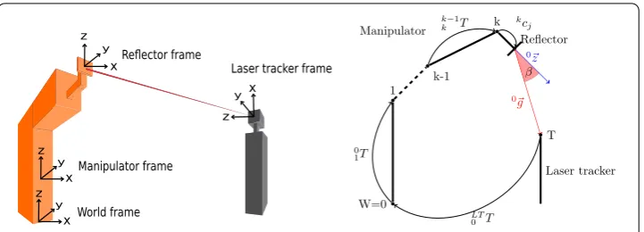
Figure 2 A laser tracker measurement system for parameter identification of industrial manipulators.

On the left, a laser tracker with a single reflector is presented. Here, the world frame is located in the foot of the manipulator. On the right, the figure shows the homogeneous transformations describing the manipulator and the laser tracker as well as the transition from the laser tracker coordinate system to the world coordinate systemLT

0 T. Transition from joint (i– 1) toiis mathematically described by the homogeneous transformationi–1

i T. The reflector is mounted on the tool center point by the translationkcj. Incident angleβbetween the reflector’s orientation vector0_{zinz-direction and the normalized laser beam} 0_{gfrom the reflector to the laser tracker is computed by (}0_zT_·0_g)· 0_g.

reflectors are mounted on the end effector of the manipulator. A laser tracker then auto-matically tracks the reflector with its laser and measures the three dimensional position of the reflector relative to the coordinate system of the laser tracker. We assume that the origin  of the world frame is located in the base of the manipulator, thatLT

 T is the

ho-mogeneous transformation from the laser tracker to the basis of the manipulator, that the manipulator hask joints and that the reflector position isk_c

i in the coordinate system

of the TCPk. In several measurement configurationsqmeas

i ,i= , . . . ,mthe laser tracker

aims its laser at the reflector and measures the position of the reflectorLT_c

i∈Rrelative

to the laser tracker coordinate system LT, e.g. by one of the following systems [, , ]. The model response relates the model position LT_c

iof the reflector in the laser tracker

coordinate system LT for theith measurement configurationqmeas_i and the TCP pose and is given by

hp,qmeas_i =LTci=LT T·TCP

p,qmeas_i ·kci∈R. ()

A measurement is considered feasible if the angle of incidenceβbetween the reflector’s orientation vectorzinz-direction (also named central rotation axis) with lengthz=  and the laser beam_{gfrom the reflector to the laser tracker with length}_{g=  is less}

than ◦, which can be described by the condition

cos◦≤cos(β) =zT·g·z·g=zT·g·g. ()

Parameter identification The solutionpˆ∈Rnp_{of the nonlinear least-squares problem,} given in the form of

min p

m

i=

 i

–_η i–hi

p,qmeas_i 

defines a local mappingpˆ=g(η,qmeas_{) which yields an estimate for the true but unknown}

parametersptrue_{. Equation () can be written more compactly as}

min p



f(p,η)



, ()

where

f:=–(η–h)∈Rm·nh_,

η:=ηT_, . . . ,η_mTT∈Rm·nh_,

h:=hT_p,qmeas_ , . . . ,h_mTp,qmeas_m bT∈Rm·nh_,

:=diag(i,i= , . . . ,m)∈Rm·nh×m·nh.

Obviously, the systematic error () can be reduced by estimatingptrue_{. Repeating the}

ex-periment leads to a different representation of measurements and thus to a different esti-matepˆ. Sinceηis a random variable,pˆ=g(η,q) is also a random variable. One can define a confidence region

CR(pˆ,α) =p: (p–pˆ)TC(p–pˆ)≤χ_n

p( –α)

containing the true parameter values to a certain probability  –α.χ

npis theχ



distribu-tion withnpdegrees of freedom.Cis the variance-covariance matrix defined by

C=FT F

–

∈Rnp×np _withF

:=

df

dp

p,qmeas.

Please note the explicit dependence of the parameter covariance matrix on the measure-ment configurations qmeas, we will write C(qmeas) to emphasize this dependence when required.

1.2 Previous work on optimum experimental design

State-of-the-art methods for parameter identification of industrial manipulators estimate the geometric parametersp∈Rnp_{by solving the nonlinear least-squares problem ().} Fit-ting the model to the measurement data by means of parameter estimation does not imply the minimization of the respective uncertainties of the resulting parameters given by the variance-covariance matrixC(qmeas_{). The quality of the parameter estimates depends on}

the choice of measurement configurationsqmeas_{. Therefore it is desired to use}

configu-rations, which provide maximal information gain and low statistical uncertainty. In that

view, the measurement configurationsqmeas _{can be optimized by solving the optimum}

experimental design (OED) problem

min qmeasφ

Cp,qmeas (a)

s.t. ≤ψp,qmeas. (b)

A cost functionφ(C(p,qmeas_{)) of the covariance matrix is minimized subject to kinematic}

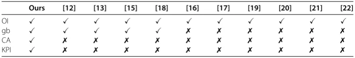
Table 1 An overview of relevant methods from the literature applied by other authors

Ours [12] [13] [15] [18] [16] [17] [19] [20] [21] [22]

OI

gb ✗ ✗ ✗ ✗ ✗ ✗

CA ✗ ✗ ✗ ✗ ✗ ✗ ✗ ✗ ✗ ✗

KPI ✗ ✗ ✗ ✗ ✗ ✗ ✗ ✗ ✗ ✗

The application of a method is marked byand its absence by✗. (OI: observability index, gb: gradient-based method, CA: collision avoidance, KPI: key performance indicator.)

• manipulator specifications,

• measurement system specifications and • collision avoidance.

The solution of the optimization problem provides measurement configurations with which a minimal uncertainty during parameter estimation is achieved. We summarize the state-of-the-art approach and give a comparative overview with respect to the methodol-ogy presented in this article in Table .

In [] and [] the quality of a given set of measurement configurations is defined by five so-called observability indices (OIs) which were first proposed byBormandMenq

in [] and []. They are based on the sensitivities w.r.t. geometric parameters and con-figurationsF:=df

dp(p,qmeas) from the parameter estimation problem (). In [] the five

quality criteria for parameter identification of industrial manipulators are related to those of OED problems []. Each of the quality criteria can be used as a cost function in the optimization problem (a)-(b).

The optimization of measurement configurations with respect to an OI achieving mini-mal parameter errors during parameter identification of industrial manipulators is an ac-tive field of research. Many solutions have been proposed which are based on derivaac-tive- derivative-free and gradient-based methods.BormandMenq[, ] present the optimization of measurement configurations with respect to the objective

max

qmeasφ=_qmaxmeas r

√_μ

·. . .·μr

√

r , ()

where μ, . . . ,μrare the singular values of F in descending order. They solve the

opti-mization problem by a steepest descent and a successive quadratic line search method. In the optimization no mechanical joint constraints are considered. In [] a conjugate gra-dient type method is used to maximize the product of singular values. In [] and [] the optimization problem

min

qmeasφ=_qminmeas

μ μr

()

is solved by a genetic algorithm and simulated annealing. During the optimization joint constraints are considered. The same objective is used in [] to compute optimized TCP poses in a constraint search space with the functionfminconfromMATLAB(The Math-works Inc.).

Daneystudied in [] the objective

min

qmeasφ=max_qmeasdet

by using tabu search. Restrictions to the sliding joints of the manipulator are considered during computation. In [] a further optimality criterion for OED is defined calledD∗ -criterion, which is adapted to the special structure of the information matrix. With regard to this criterion, optimal measurement configurations are selected from a set of config-urations. In [] theDETMAXalgorithm is used to select optimal measurement config-urations from a set of given configconfig-urations due to the objectivemaxqmeasφ_. The same algorithm is used in [] selecting optimized measurement configurations with respect to the five existing OI.

The approach of nonlinear experimental design for explicit key performance indicators (KPIs) applied to a chemical process has been discussed in [].

1.3 Contribution of the article

All presented formulations for the objective function in (a)-(b) only consider the statis-tical uncertainties of the geometric parameters of the kinematic model. We present a new optimization problem formulation in which additionally the TCP position or other KPIs are considered in the objective. Thereby, the optimization problem (a)-(b) is extended with the statistical error of TCP positions given by a number of pre-defined working con-figurations. The OED problem is solved by a sequential quadratic programming (SQP) method. The avoidance of collisions has to be considered in the optimization method to be applicable in industrial practice. This is achieved by introducing additional nonlinear con-straints to the optimization problem. The segments of the manipulator are approximated by capsules. The avoidance of collisions between two manipulator segments is described by a single nonlinear constraint in the optimization problem.

1.4 Organization of the article

In Section , we explain the methodology of OED for parameter identification of indus-trial manipulators in detail. First, we introduce the general formulation of KPIs. Second, we formulate the OED problem for KPIs. Afterwards, we introduce a collision avoidance strategy to generate collision-free measurement configurations. In Section , we present numerical results from two simulation studies. First, the KPI approach is presented for a simulation of real-world flexible measurement systems (FMS) example with three dif-ferent KUKA robots (KR, KR and KR) considering collision avoidance. Second, for a set of  different manipulator geometries the proposed methodology is statistically compared against a heuristic and a state-of-the-art method in simulation. Afterwards, the results are discussed. We finish with a conclusion and give an outlook to future work.

2 Parameter identification of manipulators with key performance indicators

In the previous section, we introduced the principle method for parameter identification of manipulators, i.e. parameter estimation using nonlinear least-squares and a kinematic model of the manipulator geometry. Furthermore, we presented linear error propagation and the quantification of the uncertainties of the geometric parameterspby means of the variance-covariance matrixC, which takes the error propagation from measurements to parameters into account, i.e.

Figure 3 An exemplary setup of a 360◦SIMS flexible measurement system.Image courtesy of Hexagon Manufacturing Intelligence.

In Section ., we presented the state of the art of optimum experimental design (OED) for parameter identification of manipulators based on the minimization of so-called ob-servability indices (OIs). This approach yields optimal measurement configurationsqmeas

maximizing the OI and with this the statistical uncertainty of the parameter estimatespˆ given byC(pˆ,qmeas_{). However, most often we are not interested in an estimate of the}

geo-metric parameters of the manipulator with a low statistical error but in having a high tool center point (TCP) precision.

In the following, we will present a mathematical concept in which the TCP precision as the main quantity of interest is explicitly considered. In the remainder of this article we will denote this main quantity of interest as key performance indicator (KPI). Primarily, we are interested in the TCP precision and, secondarily, in the precision of the geometric parameters.

In this context we use the example of flexible measurement systems (FMS) to derive the methodology of optimum experimental design for key performance indicators. In FMS an industrial manipulator measures automotive bodies, requiring a high TCP precision. An example setup is shown in Figure .

The manipulator takes measurements in the positions determined by the working con-figurationsqwork

i ∈Rk ∀i= , . . . ,tin which a high TCP precision is desired. These TCP

positions are introduced as additionals∈Rns_variables

s= TCPp,qwork ()

depending implicitly on the parameterspand the working configurationsqwork_.

Formu-lation () can be used to quantify the dependence of the KPI on parametric uncertainty by means of the explicit mappingη→p→sor the implicit mappingη→(p,s(p)).

2.1 Formulation of key performance indicators

so-called key performance indicators (KPIs). For this, the error propagation from the data

ηto the KPIssis quantified byφ(C(s)).

For given configurationsq= (qmeas,qwork)Tand related dataη, the least-squares problem () is augmented by nonlinear constraintsf∈Rn _to

min v

 f

v,qmeas,η

 (a)

s.t.  =fv,qwork (b)

with variablesv= (p,s)T_{, wheref}

∈Rmis the least-squares objective of the parameter

es-timation problem (a)-(b) andfrepresents the relation between parametersp, config-urationsqwork_{and KPIss. Specific formulations are for example the investigated precision}

of static TCP poses but also the precision of TCP path trajectories could be described. This general formulation additionally includes explicit KPI formulations like Equation (), i.e.

f={TCP(p,qworki ) –si}ti=. In the Appendix, the transformation of the constrained

least-squares problem (a)-(b) to an equivalent unconstrained problem under certain as-sumptions is derived.

Analogously to (), the solutionvˆ= (pˆ,sˆ)T _{of the constrained nonlinear least-squares}

problem (a)-(b) is subject to statistical uncertainty due to the stochasticity of the measurement data η. The propagated uncertainty for both, the parameter and the KPI estimatespˆ,ˆs, can be considered for the minimization in OED.

In the following, we give the required definitions and assumptions to formulate the OED problem for KPIs. Assume in the following discussion that

F:=

d

dvf(v,q,η)∈R

m×nv _{and F}

:=

d

dvf(v,q)∈R

n×nv_{, ()}

satisfy the regularity conditions

(CQ) rank(F) =n and (PD) rank(J) =nv, ()

J= (FT

,FT)T∈R(m+n)×nv.

As for the unconstrained least-squares problem, one can describe a confidence region of the solutionvˆ. The statistical uncertainty of the measurementsη∈Rm_{is propagated to}

the estimated parameters. We denote the mapping from measurement dataηto estimated quantitiesvˆ, including the KPIs, by

gv:Rm→Rnv

η→ ˆv=gv(η;q),

()

the solution of the constrained least-squares problem (a)-(b) withq= (qmeas_,qwork_).

It is well-known that for a normally distributed random variable X ∼ N(μ,) an

affine mapping Y =g(X) =AX+b yields another normally distributed random

vari-able Y ∼N(Aμ+b,A_AT_{). For nonlinear functions one can linearize the function}

and use the linear error propagation approximation. Thus, forgvthe random variable V∼N(gv(η;q),dgv

dη(η;q) d

gv

Lemma Under the assumptions(CQ), (PD),it holds that

v=dgv

dη(η;q)η ()

=I 

FT

F FT F 

– FT

 –



η, ()

whereI∈Rnv×nv_,F

≡F(η,q),F≡F(q)andv:=v–vˆ,η:=η–ηˆdenote the respective differences between current and expected values.

Proof See [].

In the following,E(·) denotes the expected value of a random variable. From this Lemma it follows that

Cv=EvvT

=I 

FT

FFT F 

– FT

 F 

 

FT F FT

F 

–T I



.

The formula can be shown to be equivalent to Equation ():

Proposition The variance-covariance matrix Cv:=E((v–Ev)(v–Ev)T_)satisfies

Cv=

Cp Cps Csp Cs

=I 

FT

F FT

F 

– I



. ()

Proof See [].

2.2 Collision avoidance

In the following, we present a collision avoidance strategy required for the practical real-ization of OED for KPIs in industrial applications. The optimized measurement configu-rationsqmeas_{are required to be free of collisions between the manipulator and its}

environ-ment. This is achieved by introducing a collision avoidance strategy to the formulation of the OED problem.

We give an overview of existing collision avoidance approaches. Afterwards, our ap-proach is presented in a general manner for the fact that the collision avoidance formula-tion is not restricted to flexible measurement systems. In Secformula-tion . the collision avoid-ance technique is then applied on a specific experimental setting.

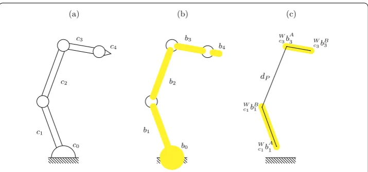
Figure 4 Visualization of the capsule approximation.Each jointci,i∈ {0,. . ., 4}in column(a)is described by an appropriate capsulebi,i∈ {0,. . ., 4}illustrated in column(b). In column(c)the distancedPbetween the two line segmentsb1andb3is shown.

The shapes of industrial manipulators are less complex than those of humanoid robots. Therefore, we follow the approach from [], where the industrial manipulator as well as the obstacles in the working environment are approximated by spheres and capsules. The approximation process is exemplarily visualized in Figures (a) and (b). Hereby, each link

cof the manipulator is described by appropriate capsulesbi=Capsule(W_c bA_i,W_c bB_i,ri),i∈R, whereRis the index set of all manipulator specific capsules. Each capsule consists of a radiusri and its end pointsW

c bAi,Wc bBi ∈R for the manipulator segmentcin the world

coordinate systemWgiven by

W c bAk =

c

i= i–

i T(pi,qi)·cbAk and Wc bBk= c

i= i–

i T(pi,qi)·cbBk.

Similarly, each object is approximated by a capsulebj=Capsule(W_bA

j,WbBj,rj),j∈Owith

the index set of all environment specific capsulesO.

A configuration is collision-free when the distance between each pair of capsules is larger than zero. The distance between two capsulesbandbof two different jointsc

andccan be computed by

d(b,b) =dP(b,b) – (r+r)≥ ()

with

dP(b,b) = 

i= _W

cbBi–WcbAi

t–W

cbBi–WcbAi

u–W

cbAi+WcbAi 

, t,u∈R, ()

which computes the distance of the two respective line segments, cf. Figure (c).Lumelsky

introduced an algorithm to compute the distancedPbetween two line segments in [].

into points or if the line segments are parallel. If none of the cases holds, the minimal distance is computed using a parameterized formulation of the line segments. Follow-ing this, a nonlinear constraint like () for each pair of considered capsules is formu-lated in the optimization problem which guarantees optimized, collision-free configura-tions.

If the manipulator consists ofnsegments each approximated by a single capsule, the maximal number of constraints for collision avoidance can be computed by the formula

max # of constraints =n(n– )

 – (n– ). ()

Two neighboring segments do not have to be compared as the limitation of joint move-ment automatically prevents their collision.

Not all segments can be described by just one suited capsule. If the first or last joint is described bykcapsules, then additionally (k– )·(n– ) constraints have to be added to (). If one of the interior segments is described bykcapsules this results in (k– )·(n– ) additional constraints. The total number of constraints can be decreased by further in-vestigation of the geometry of the manipulator and motion to find segments which will never collide and therefore do not have to be considered in the collision avoidance strat-egy. A study in [] has shown, that the blow up from inlying to enclosing capsules only has a slightly negative influence on the optimization performance. As the descrip-tion of an industrial manipulator by capsules is just an approximadescrip-tion of reality, the use of enclosing capsules guarantees by higher probability that the optimized measurement configurations are collision-free in a practical application without losing much perfor-mance.

Analyzing the derivative of () w.r.t. the control variablesqyields that the first fraction has a singularity if the distance between two line segments becomes zero. But this will never be the case as in each constraint the distance of line segments must be equal or larger than the sum of the capsules’ radii.

dd(b,b)

dq =



_i=[(W

c bBi–Wc biA)t– (Wc bBi–cWbAi)u–Wc bAi+Wc bAi]

· _∂ 

∂q 

i=[(Wc bBi–Wc bAi)t– (Wc bBi–Wc bAi)u–Wc bAi+Wc bAi]

· _∂ 

∂q(Wc bBi–cWbAi)t– (Wc biB –Wc bAi)u–Wc bAi+Wc bAi

. ()

2.3 Optimum experimental design for key performance indicators

We now assemble the problem formulation of OED for KPIs considered in this arti-cle. A function of the variance-covariance matrix C(qmeas_{) is minimized to find}

opti-mal measurement configurations for the parameter identification procedure. Depending on the choice of the objective, either the parametric uncertainty of the geometric pa-rameters and/or the KPIs is minimized. The explicit dependence ofC(qmeas_{) can be}

OED problem

min qmeastr

PTCv(q)P (a)

s.t. ≤ψp,qmeas ⎧ ⎪ ⎪ ⎪ ⎪ ⎪ ⎨ ⎪ ⎪ ⎪ ⎪ ⎪ ⎩

qlo_i ≤qmeas_i ≤q_iup, i= , . . . ,k, (_zT_·_g)· _{g ≤cos(}◦_),

d(bi,bj)≥, i,j∈R,{i,j}∈/I,

d(bi,bj)≥, i∈R,j∈O

(b)

withCv=

I 

FT

 F FT

F 

– I



, (c)

F=– d

dvh

p,qmeas and (d)

F= d dvTCP

p,qwork. (e)

Pis a matrix projecting onto a subset ofp, ofsor ofpandswith the possibility to scale each parameter independently.Iis a set of manipulator segment indices, which do not have to be compared for collision avoidance. The variance-covariance matrixCvresults

from the constrained parameter estimation problem (a)-(b) with derivativesFand

F as introduced in Section .. As objective function (a) we choose the arithmetic mean of the diagonal element of the projected variance-covariance matrix, the so-called A criterion, corresponding to the average of the half-axes of the confidence ellipsoid, see []. The constraintsψ(p,qmeas_{) include restrictions for the movement of each jointi,}

the incident angle between laser beam and the orientation vector of the TCP inz direc-tion and the collision avoidance between manipulator segments and between manipula-tor segments and obstacles. In problem (a)-(e) the control variablesqwork_{are fixed}

defining the TCP pose during the work process and only the measurement configura-tions qmeasare optimization variables. As problem (a)-(e) does not depend on the dataη, optimal experimental designs can be computed before the experiments are carried out.

3 Numerical results

The task of a manipulator in flexible measurement systems is to detect small production errors. Hence a high precision at the tool center point (TCP) of the manipulator is re-quired. The precision is improved by sequentially identifying the manipulator’s parame-ters in a fixed time interval, e.g. after each work cycle of the manipulator. The work cycle consists of one working configurationqwork_∈R_{after which the re-identification of the}

Table 2 Denavit-HartenbergandHayatizero offset values withλ∈ {650, 700, . . . , 1,050}and

μ∈ {600, 650, . . . , 1,050}

Jointi θi(◦) αi(◦) ai(mm) di(mm) βi(◦)

1 0.00 90.00 350.00 0.00

-2 0.00 0.00 0.00 - λ

3 –90.00 90.00 145.00 0.00

-4 0.00 –90.00 0.00 μ

-5 0.00 90.00 0.00 0.00

-6 180.00 180.00 0.00 –170.00

-Zero offsets of the underlined values are considered in OED.

Table 3 Position and orientation of laser tracker and reflector

Laser tracker Reflector (k_c j)

x(mm) 2,730.88 –89.58

y(mm) 4,554.68 –2.84

z(mm) 1,397.67 327.03

α(◦) –95.63

-β(◦) –95.63

-γ(◦) 0.23

-projections

Cp=I Cv

I



and Cs= ICv



I

, ()

withI∈Rnp×np_andI∈Rns×ns_{considered in the cost function of the optimization} prob-lem. Covariance matrixCp only considers the statistical uncertainties of the geometric parameters, whileCsconsiders the uncertainties of the KPI only. The OED problems are solved with the parameter values presented in Table  and Table . Please note that no parameter estimations are performed. In both tables, we highlight the parameters whose uncertainties are considered in the optimization. The different tasks in thein-silico exper-iment are depicted by Figure , which gives an overview of the work flow of the parameter identification process. In the following all tasks are performed to compute optimal sets of configurations for the current parameter identification.

3.1 Software

The optimization problem is solved with the software packageVPLAN[], developed in the research group of the authors. The evaluation of derivatives is performed byADIFOR

[].ADIFORis able to evaluate the derivatives of the vector-valued objective function (). The OED problem (a)-(e) is formulated as a nonlinear optimization problem and solved by the sparse SQP solverSNOPT[].

3.2 Experimental setup

Figure 5 Overview of the parameter identification procedure under consideration.The figure shows the general approach to parameter identification of industrial manipulators and mechanisms using KPIs. We assume the manipulator has to perform a measurement task on certain TCP positionssrequiring a high precision. These positions are considered as KPIs for the parameter identification procedure. The required precision is achieved by combining a (re-)identification of the parameters with the actual work cycle of the manipulator, i.e. whenever the manipulator is idle it can sequentially identify itself. Both the measurement and parameter identification task take place in the same scene. From scene and manipulator model the necessary obstacle descriptions are required to setup the collision avoidance for the OED problem. The OED problem will find an optimal set of configurationsqfor the optimization problem considering the collision avoidance and the chosen KPI from a given set of initial configurations. Whenever the manipulator performs an identification task, the internal kinematic model is updated with the current optimal parameter valuesptrue.

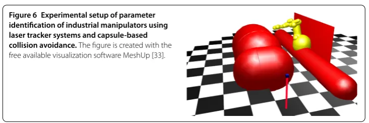
Figure 6 Experimental setup of parameter identification of industrial manipulators using laser tracker systems and capsule-based collision avoidance.The figure is created with the free available visualization software MeshUp [33].

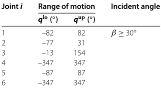
Table 4 Range of motion of joints and admitted incident angle between sensor surface and laser beam

Jointi Range of motion Incident angle

qlo₍◦_{) q}up₍◦₎

1 –82 82 β≥30◦

2 –77 31

3 –13 154

4 –347 347

5 –87 87

6 –347 347

to the TCP of the manipulator. Its positionk_c

j in the TCP coordinate systemk, cf.

Ta-ble , is not exactly known and will be estimated as well. The pose of the laser tracker is summarized in Table  and will also be identified during the parameter identification. The measurement erroriof the laser tracker depends on the precision with which the laser

tracker can determine the wavelength of light in the measurement environment (cf. []). In [] an expanded uncertainty (k= ) of μm + .μm on reference length measure-ments up to  m is achieved using a laser tracker in their tape tunnel facility. Please note that we are performing anin-silicoexperiment to draw the attention to the performance of our new method. Therefore, we assume

i∼N ⎛ ⎜ ⎝ ⎡ ⎢ ⎣    ⎤ ⎥ ⎦, ⎡ ⎢ ⎣          ⎤ ⎥ ⎦ ⎞ ⎟

⎠, i= , . . . , .

The ranges of manipulator motions are defined by the upper and lower bounds of the manipulator specific control variablesθ, . . . ,θlisted in Table . As we are using a laser

tracker system the only system dependent constraint is the restricted angle of incidence between the sensor surface and the laser beam, cf. Table .

The constraints which are needed during optimization to avoid collisions are discussed in the following. The work space of the manipulator is constrained by a wall behind the manipulator imposing constraints

_W c bAi

x–ri≥–., _W

c bBi

x–ri≥–.

∀i∈Rinxdirection. The manipulator is not supposed to hit the ground. Therefore, we impose constraints

_W c bAi

z–ri≥., _W

c bBi

z–ri≥.

∀i∈Rthat guarantee positivez positions for all manipulator bodies. Auto-collision is avoided by constraints between several manipulator bodies. The distance between the manipulator bodies and the object to which the manipulator is mounted should also be positive. The car, whose body should be measured, is modeled by two capsules, which are not allowed to collide with the manipulator parts.

Table 5 Values of the constraints to avoid collisions between manipulator bodies, laser beam and object bodies

Manipulator bodies (mm) Laser beam (mm)

xdirection ≥450.0

-ydirection -

-zdirection ≥0.0

-Manipulator bodies ≥0.0 ≥0.0

Object ≥0.0

-Car part 1 ≥0.0 ≥0.0

Car part 2 ≥0.0 ≥0.0

Table 6 Key performance indicator (KPI) average variances (mm2) of three KUKA robots with heuristic and optimized experimental designs for parameter identification

Cost function Average variance of KPI (mm2):1₃tr(Cs)

Heuristic Optimized with collision avoidance

φA(Cp) φA(Cs)

KR 15 0.59 0.40 0.33

KR 300 0.58 0.39 0.35

KR 500 0.61 0.40 0.35

Heuristic Standard method KPI method

Optimizations are performed with different cost functions.

The radii of the capsules are chosen in a way, that the capsules nearly surround their appropriate manipulator segments. The surrounding capsules are used as a conservative and robust approach to guarantee that the optimized measurement configurations are applicable in reality. Each simulated parameter identification consists of  measurement configurations from a heuristic approach and from the optimization method introduced in Section .. The  heuristic measurement configurations are randomly and uniformly chosen from the motion range of the industrial manipulator. In the experiment two sets of measurement configurations are computed differing by the choice of variance-covariance matrix projections in the cost function of optimization.

3.3 Computation of optimum experimental designs

.. KUKA robots(KR,KR,KR)

Firstly, three types of KUKA robots (KR, KR, KR) [] are considered in simula-tion with the experimental setting introduced in Secsimula-tion .. Due to the different mechan-ical shapes also the number of capsules describing the manipulator segments differ and accordingly the number of collision avoidance constraints are  for the KR,  for the KR and  for the KR. Heuristic and optimized measurement configurations for the parameter identification of three KUKA robots are considered. The measurement configurations are optimized with the two different variance-covariance matrix projec-tions, cf. () and with consideration of collision avoidance. The resulting average statisti-cal uncertainties of the TCP precision by either using heuristic or optimized measurement configurations for parameter identification are shown in Table .

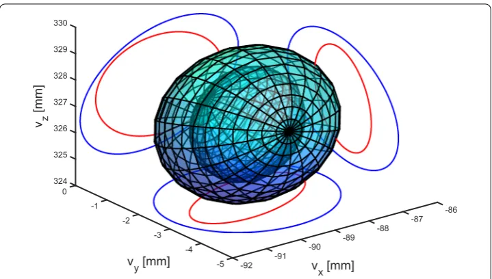
Figure 7 Error ellipsoid defining the linearized 95% confidence region of the tool center point (TCP) of the working configuration.Error ellipsoid defining the linearized 95% confidence region (with χ2

3(0.95) = 7.815) of the TCP of the working configuration of a KUKA KR15 with its two dimensional projections resulting from heuristicqhand optimizedqsmeasurement configurations used in parameter identification. The center of the ellipsoid is the TCP position with its parameter values presented in Table 3. The half-axesvx,vy,vzof the confidence ellipsoids are the eigenvalues of the covariance matricesCs(qh) (blue) andCs(qs) (red) withqs:= minqtr(Cs(q)).

.. Variety ofindustrial manipulators

For a quantitative analysis, simulated parameter identifications are performed with  notional industrial manipulators. Figure  presents a comparison of the average variances of the TCP between the new approach using a KPI and (a) the heuristic approach and (b) the state-of-the-art optimization approach. During optimization collision avoidance is considered. Higher values on thex-axis mean a better result of our approach using a KPI. We also computed optimized experimental designs without consideration of colli-sion avoidance during optimization. % to % of the measurement configurations lead to collisions so that the designs are not applicable in practice. The minimum and maxi-mum value of the averaged three dimensional variances of the TCP from the  different experiments are shown in Table .

In Table  the heuristic and optimized average variances of the TCP of the working configuration for the  experiments due to the four different experimental designs and the use of the collision avoidance method in the optimization are shown.

4 Discussion

4.1 KUKA robots (KR15, KR300, KR500)

In the simulated parameter identification of the three different KUKA robots, the opti-mized experimental designsqmeas

p andqmeass provide higher TCP accuracies in contrast

to the heuristic experimental design (improvement of % to %). The largest improve-ment of the precision of the TCP is achieved by only using the covariance matrixCsof

Figure 8 Kernel density estimations of the position precision of the tool center point (TCP) between the new approach using key performance indicator and (a) the heuristic approach and (b) the state-of-the-art optimization approach.The Histogram presents the difference of TCP precision of working configurationqwork_{from the new approach using KPI and the heuristic/state-of-the-art optimized}

measurement configurationsqmeas

x , wherex∈ {h,p}for 90 parameter identifications differing in the industrial manipulators’ models. Higher values on thex-axis mean a better result of the new approach. The optimized measurement configurationsqpandqsresult by solving the optimization problems:

qmeasp := minqmeastr(Cp(qtotal)) andqmeass := minqmeastr(Cs(qtotal)).

Table 7 Minimum and maximum value of the averaged three dimensional variances of the tool center point (mm2) from the 90 experiments with heuristic and optimized experimental design for parameter identification

Cost function Range of KPI average variance (mm2)

Min Max Min Max

Heuristic - - 0.55 0.71

φA(Cp) 0.39 0.39 0.42 0.45

φA(Cs) 0.33 0.34 0.34 0.37

Collision avoidance No Yes

Optimization is performed with different cost functions.

account, yields a higher TCP precision (KR : %, KR : %, KR : %). Moreover, our formulation of optimizing measurement configurations can be used for industrial ma-nipulators with a low payload to heavy duty models.

4.2 Variety of 90 industrial manipulators

Table 8 Key performance indicator (KPI) average variances (mm2) of 90 experiments with heuristic and optimized experimental design for parameter identification

Cost function Average variance of KPI (mm2_):1 3tr(Cs)

Heuristic Optimized Optimized

φA(Cp) 0.61 0.39 0.43

φA(Cs) 0.61 0.33 0.35

Collision avoidance - No Yes

Optimization is performed with different cost functions.

configurations, has an increasing effect on the optimization performance by % to %. Table  indicates that the largest improvement (%) of the TCP precision is achieved by only using the statistical uncertainty of the TCP position as cost function. Moreover, the case study stresses that the new approach using KPIs is superior to the state-of-the-art optimization approach providing a % higher TCP precision on average. The case study underlines the benefit of the TCP precision achieved through our problem formulation and shows that the improvement is not limited on specific KUKA models but on a range of small to large industrial manipulators.

5 Conclusion

This article introduces a new problem formulation for the computation of optimal and collision-free measurement configurations for parameter identification of industrial ma-nipulators. The novelty lies in the fact, that the precision of the tool center point (TCP) is directly considered in the optimization problem as a key performance indicator (KPI). The approach is verified by the simulated parameter identification of three different KUKA robots and also by the quantitative results with  notional manipulator geometries. In the experiments an improvement of % to % of the precision of the TCP is achieved in contrast to the heuristic approach and % to % improvement compared to an existing state-of-the-art method. For the computation of collision-free configurations required in practice a collision avoidance method is introduced, which provides a minimal number of nonlinear constraints in the optimization problem. In the experiments a laser tracker system is used for parameter identification but the approach is also applicable to other measurement systems. Furthermore, the approach is not limited to a specific observability index (OI) as cost function. As our approach yields a higher TCP precision with the same number of measurement configurations it is also possible to reduce the needed number of configurations to achieve a certain TCP precision in a shorter re-identification time interval compared to the heuristic approach.

6 Outlook

in re-identification and a higher throughput. Additionally, the online parameter identifi-cation has the advantage that the parameter identifiidentifi-cation can be stopped when a certain level of TCP precision is reached which results in shorter parameter identification inter-vals.

At the moment, the improvements are achieved by considering a kinematic model of the manipulator only. However, the improvement could be increased by incorporating a higher level of detail of the manipulator into the model. The higher level of detail is achieved by introducing further parameters, e.g. non-geometric errors like joint mobili-ties or elasticimobili-ties. This would require the computation of forces acting on the links and joints, which can be achieved by using a dynamic model of the manipulator described by differential equations. As shown in [], the same approach for differential equation models can be used when the required derivative information is available. However, this approach is yet to be investigated for the dynamics of multi-body systems acting as dy-namic model for the parameter identification procedure.

Another possible extension is the definition and consideration of further KPIs in the optimization problem. The article demonstrates that the use of TCP precision as KPI achieves a significant precision improvement after parameter identification over the heuristic parameter identification approach as well as the existing state-of-the-art prob-lem formulations not using KPIs. Future work will investigate the possibilities of not only taking one TCP pose into account but additional poses of important working configura-tions. Furthermore, the definition of KPIs is not limited to TCPs, such that working path trajectories of welding manipulators could be defined as KPIs as well. This way, the range of possible application of the proposed approach will be increased.

Appendix

A.1 A comparison between constrained and unconstrained least-squares

In the Appendix, we discuss an alternative approach to tackle key performance indicators (KPIs). Due to the (CQ) condition, the constrained least-squares problem (a)-(b) can be reformulated as an unconstrained least squares problem by parametrization of thes variables. By application of the implicit function theorem there exists an unique solution

s=(p) :=s∈Rn

s| =f(p,s)

.

and hence (a)-(b) can be written as

min p∈Rnp

 f

p,(p);η,q

.

The Jacobian off˜(p;η,q) :=f(p,(p);η,q) is

˜

F=d˜f dp=

∂f ∂p+

∂f

ds(p,s;η,q)

"" ""

s=(p)

d

dp

=∂f

∂p+

∂f

∂s(p,s;η,q)

"" ""

s=(p) #

∂f ∂s

For notational simplicity we define

A B:=F=

%

∂f ∂p

∂f ∂s &

,

E F:=F= %

∂f ∂p

df ∂s &

and thus

˜

F=A+BF–E.

The covariance matrix of the unconstrained parameter estimation problem is therefore

˜

Cp=F˜_TF˜ –

=A+BF–ETA+BF–E–.

To obtain the covariance matrix of the KPIsone can apply linear error propagation and finds

˜

Cs=F–ECp˜ F–ET.

The following two propositions show thatCp˜ =CpandCs˜ =Cs.

Proposition Let(CQ)and(PD)be satisfied and let the columns of Z∈R(nv–n)×nv _span

the null-space of F,i.e.,

FZ= .

Then it holds that

I 

FT

F FT

F 

– I



=ZTZF_TFZT –

Z.

Proof

FT

F FT

F 

– I



=

C D

(a)

⇔ I=F_TFC+F_TD, (b)

 =FC. (c)

From (c) and the condition (CQ) one concludes that there exists aK of matching di-mensions satisfyingC=ZK. Inserting this identity into (b) and multiplication byZT

from the left one obtains

From condition (PD) it follows thatZT_FT

FZis non-singular and thus

K=ZTF_TFZ–ZT

⇔ C=ZZTF_TFZ–ZT

by multiplication ofZfrom the left. This is the desired result.

Proposition Let Cp,Cs,Cp˜ andCs˜ be defined as above.It holds that

˜

Cp=Cp and Cs˜ =Cs.

Proof We apply the result of the latter Proposition with the specific matrix

ZT=

I

–F–_E

yielding

Cp=ZF_TFZT–

=

'

I (–F–_E)TT

AT_{A A}T_B BT_{A B}T_B

I

(–F–_E)T (–

=

'

I (–F–_E)TT

AT_A–AT_BF–_E BT_A–BT_BF–_E

(–

=ATA–F–ETBTA+F–ETBTBF–E–

=A+BF–ETA+BF–E–

=Cp˜

and

Cv=ZTZF_TFZT–Z

=

Cp –Cp(F–E)T

–F–ECp (F–E)Cp(F–E)T

.

Projecting onto thesvariables results in

Cs= ICv



I

=F–ECpF–ET

Funding

S Körkel, SF Walter and M Kudruss were financially supported byBASF SE. F Jost and M Kudruss were supported by DFG Graduate School 220Heidelberg Graduate School of Mathematical and Computational Methods for the Sciencesfunded by the German Excellence Initiative. The authors thankfully acknowledge the financial support of theDeutsche

ForschungsgemeinschaftandRuprecht-Karls-UniversitätHeidelberg within the funding programmeOpen Access Publishing.

Abbreviations

KPI: key performance indicator; OI: observability index; OED: optimum experimental design; TCP: tool center point.

Competing interests

The authors declare that they have no competing interests.

Authors’ contributions

SK developed the software VPLAN implementing the numerical methods for nonlinear experimental design used for the computations in this article. He formulated the idea of optimum experimental design for explicit KPIs. MK extended the idea to the implicit formulation and was responsible for the efficient implementation in VPLAN as well as the geometric manipulator model. SFW together with MK developed the connection of the covariance matrix of the constrained and unconstrained OED problems with KPIs. FJ devised the problem setups, implemented the collision avoidance strategy and realized the computations for the numerical results. FJ wrote major parts of the manuscript and was supported by MK and SFW with suggestions, fine-tuning and proofreading.

Author details

1_{Otto-v.-Guericke-University Magdeburg, Universitätsplatz 2, 02-204, 39106 Magdeburg, Germany.}2_{Interdisciplinary} Center for Scientific Computing, Heidelberg University, Im Neuenheimer Feld 205, 69120 Heidelberg, Germany. 3_{Ostbayerische Technische Hochschule Regensburg, Postfach 12 03 27, 93025 Regensburg, Germany.}

Publisher’s Note

Springer Nature remains neutral with regard to jurisdictional claims in published maps and institutional affiliations.

Received: 27 April 2016 Accepted: 26 June 2017 References

1. World Robot Statistics. International Federation of Robotics (IFR). 2014.

2. Denavit J, Hartenberg RS. A kinematic notation for lower-pair mechanisms based on matrices. J Appl Mech. 1955;22:215-21.

3. Hayati S, Mirmirani M. Improving the absolute positioning accuracy of robot manipulators. J Robot Syst. 1985;2(4):397-413.

4. Mooring WB, Roth SZ, Driels MR. Fundamentals of manipulator calibration. 1991.

5. Nubiola A, Bonev IA. Absolute calibration of an ABB IRB 1600 robot using a laser tracker. Robot Comput-Integr Manuf. 2013;29:236-45.

6. Park I, Lee B, Cho S, Hong Y, Kim J. Laser-based kinematic calibration of robot manipulator using differential kinematics. IEEE/ASME Trans Mechatron. 2012;17(6):1059-67.

7. Elatta AY, Gen LP, Zhi FL, Daoyuan Y, Fei L. An overview of robot calibration. Inf Technol J. 2004;3(1):377-85. 8. Nubiola A, Slamani M, Joubair A, Bonev IA. Comparison of two calibration methods for a small industrial robot based

on an optical CMM and a laser tracker. Robotica. 2013;32(3):447-66.

9. Santolaria J, Majerena AC, Samper D, Brau A, Velázquez J. Articulated arm coordinate measuring machine calibration by laser tracker multilateration. Sci World J. 2014;2014:681853.

10. Sun Y, Hollerbach MJ. Determination of optimal measurement configurations for robot calibration based on observability measure. In: International conference on robotics and automation. 2008.

11. Joubair A, Bonev AI. Comparison of the efficiency of five observability indices for robot calibration. Mech Mach Theory. 2013;70:254-65.

12. Borm JH, Menq C. Experimental study of observability of parameter errors in robot calibration. In: Proceedings of the IEEE international conference on robotics and automation. 1989.

13. Borm JH, Menq C. Determination of optimal measurement configurations for robot calibration based on observability measure. Int J Robot Res. 1991;10(1):51-63.

14. Pukelsheim F. Optimal design of experiments. New York: Wiley; 1993.

15. Khalil W, Gautier M, Enguehard C. Identifiable parameters and optimum configurations for robots calibration. Robotica. 1991;9(1):63-70.

16. Zhuang H, Wu J, Huang W. Optimal planning of robot calibration experiments by genetic algorithms. In: Proceedings of the IEEE international conference on robotics and automation. 1996.

17. Zhuang H, Wang K, Roth ZS. Optimal selection of measurement configurations for robot calibration using simulated annealing. In: Proceedings of the IEEE international conference on robotics and automation. 1994.

18. Park J, Kim S, Ryu J. Determination of identifiable parameters and selection of optimum postures for calibrating Hexa Slide manipulators. In: ICCAS. 2003.

19. Daney D, Papegay Y, Madeline B. Choosing measurement poses for robot calibration with the local convergence method and tabu search. Int J Robot Res. 2005;24(6):501-18.

20. Klimchik A, Wu Y, Caro S, Pashkevich A. Design of experiments for calibration of planar anthropomorphic manipulators. In: International conference on advanced intelligent mechatronics. 2011.

22. Joubair A, Zhao LF, Bigras P, Bonev I. Absolute accuracy analysis and improvement of a hybrid 6-DOF medical robot. Ind Robot. 2015;42(1):44-53.

23. Körkel S, Arellano-Garcia H, Schöneberger J, Wozny G. Optimum experimental design for key performance indicators. In: Braunschweig B, Joulia X, editors. Proceedings of 18th European symposium on computer aided process engineering - ESCAPE 18. 2008.

24. Bock HG, Körkel S, Kostina E, Schlöder JP. In: Jäger W, Rannacher R, Warnatz J, editors. Robustness aspects in parameter estimation, optimal design of experiments and optimal control. Berlin: Springer; 2007. p. 117-46. 25. Gerdts M, Henrion R, Hömberg D, Landry C. Path planning and collision avoidance for robots. Numer Algebra Control

Optim. 2012;2(3):437-63.

26. Stasse O, Escande A, Mansard N, Miossec S, Evrard P, Kheddar A. Real-time self collision avoidance task on a HRP-2 humanoid robot. In: IEEE international conference on robotics and automation. 2008.

27. Bosscher P, Hedman D. Real-time collision avoidance algorithm for robotic manipulators. Ind Robot. 2009;38(2):186-97.

28. Lumelsky JV. On fast computation of distance between line segments. Inf Process Lett. 1985;21(2):55-61. 29. Jost F. Optimum experimental design for parameter estimation of kinematic chains with consideration of collision

avoidance [Master’s thesis]. Heidelberg: Heidelberg University; 2015.

30. Körkel S. Numerische Methoden für optimale Versuchsplanungsprobleme bei nichtlinearen DAE-Modellen [PhD thesis]. Heidelberg: Universität Heidelberg; 2002.

31. Bischof C, Khademi P, Mauer A, Carle A. Adifor 2.0: automatic differentiation of Fortran 77 programs. IEEE Comput Sci Eng. 1996;3(3):18-32.

32. Gill PE, Murray W, Saunders MA. SNOPT: an SQP algorithm for large-scale constrained optimization. SIAM J Optim. 1997;12:979-1006.

33. Felis M. MeshUp. 2012. https://bitbucket.org/MartinFelis/meshup. Accessed 17 Jan 2017.

34. Muralikrishnan B, Phillips S, Sawyer D. Laser trackers for large-scale dimensional metrology: a review. Precis Eng. 2016;44:13-28.