R E S E A R C H
Open Access
Line search fixed point algorithms based
on nonlinear conjugate gradient directions:
application to constrained smooth convex
optimization
Hideaki Iiduka
**Correspondence: [email protected]
Department of Computer Science, Meiji University, 1-1-1 Higashimita, Tama-ku, Kawasaki-shi, Kanagawa, 214-8571, Japan
Abstract
This paper considers the fixed point problem for a nonexpansive mapping on a real Hilbert space and proposes novel line search fixed point algorithms to accelerate the search. The termination conditions for the line search are based on the well-known Wolfe conditions that are used to ensure the convergence and stability of
unconstrained optimization algorithms. The directions to search for fixed points are generated by using the ideas of the steepest descent direction and conventional nonlinear conjugate gradient directions for unconstrained optimization. We perform convergence as well as convergence rate analyses on the algorithms for solving the fixed point problem under certain assumptions. The main contribution of this paper is to make a concrete response to an issue of constrained smooth convex optimization; that is, whether or not we can devise nonlinear conjugate gradient algorithms to solve constrained smooth convex optimization problems. We show that the proposed fixed point algorithms include ones with nonlinear conjugate gradient directions which can solve constrained smooth convex optimization problems. To illustrate the practicality of the algorithms, we apply them to concrete constrained smooth convex optimization problems, such as constrained quadratic programming problems and generalized convex feasibility problems, and numerically compare them with previous algorithms based on the Krasnosel’ski˘ı-Mann fixed point algorithm. The results show that the proposed algorithms dramatically reduce the running time and iterations needed to find optimal solutions to the concrete optimization problems compared with the previous algorithms.
MSC: 47H10; 65K05; 90C25
Keywords: constrained smooth convex optimization; fixed point problem;
generalized convex feasibility problem; Krasnosel’ski˘ı-Mann fixed point algorithm; line search method; nonexpansive mapping; nonlinear conjugate gradient methods
1 Introduction
Consider the followingfixed point problem(see [], Chapter , [], Chapter , [], Chap-ter , [], ChapChap-ter ):
Findx∈Fix(T) :=x∈H:Tx=x, (.)
where H stands for a real Hilbert space with inner product·,· and its induced norm
· ,Tis anonexpansivemapping fromHinto itself (i.e.,T(x) –T(y) ≤ x–y(x,y∈ H)), and one assumesFix(T)=∅. Problem (.) includes convex feasibility problems [], [], Example ., constrained smooth convex optimization problems [], Proposition ., problems of finding the zeros of monotone operators [], Proposition ., and monotone variational inequalities [], Subchapter ..
There are useful algorithms for solving Problem (.), such as theKrasnosel’ski˘ı-Mann algorithm[], Subchapter ., [], Subchapter ., [–], theHalpern algorithm[], Sub-chapter ., [, ], and thehybrid method[] (Solodov and Svaiter [] proposed the hybrid method to solve problems of finding the zeros of monotone operators). This paper focuses on the Krasnosel’ski˘ı-Mann algorithm, which has practical applications, such as analyses of dynamic systems governed by maximal monotone operators [] and nons-mooth convex variational signal recovery [], defined as follows: given the current iterate xn∈Hand step sizeαn∈[, ], the next iteratexn+of the algorithm is
xn+:=xn+αn
T(xn) –xn
. (.)
Assuming that (αn)n∈Nsatisfies the condition
∞
n=
αn( –αn) =∞, (.)
the sequence (xn)n∈Ngenerated by Algorithm (.) weakly converges to a fixed point ofT (see,e.g., [], Theorem .). This result indicates that Algorithm (.) with constant step sizes (e.g.,αn:=α∈(, ) (n∈N)) or diminishing step sizes (e.g.,αn:= /(n+ ) (n∈N)) can solve Problem (.). Propositions and in [] indicate that Algorithm (.) with condition (.) has the following rate of convergence: for alln∈N,
xn–T(xn)=O n
k=
αk( –αk) –
(.)
(e.g.,xn–T(xn)=O(/
√
n+ ) whenαn:=α∈(, ) (n∈N)). This fact implies that Al-gorithm (.) with (.) does not always have fast convergence and has motivated the de-velopment of modifications and variants for the Krasnosel’ski˘ı-Mann algorithm in order to accelerate Algorithm (.).
One approach to accelerate Algorithm (.) with (.) is to develop line search meth-ods that can determine a more adequate step size than a step size satisfying (.) at each iterationnso that the value ofxn+–T(xn+)decreases dramatically. Magnanti and
Per-akis proposed anadaptive line search framework[], Section , that can determine step sizes to satisfy weaker conditions [], Assumptions A and A, than (.). On the basis of this framework, they showed that Algorithm (.), with step sizesαnsatisfying the follow-ingArmijo-typecondition, converges to a fixed point ofT [], Theorems and : given xn∈RN,β > ,D> , andb∈(, ), choose the smallest nonnegative integer lnso that αn=blnsatisfies the condition
gn(αn) –gn()≤–DblnT(xn) –x
n
wheregn: [, ]→Ris a potential function [], Scheme IV, defined for allα∈[, ] by
gn(α) :=xn+α
T(xn) –xn
–Txn+α
T(xn) –xn
–βα( –α)T(xn) –xn. (.)
Theorem in [] shows that Algorithm (.) with the Armijo-type condition (.) satisfies
xn+–T(xn+)≤[–β(αn–/)]xn–T(xn)(n∈N), which implies that the algorithm has, for alln∈N,
xn–T(xn)=O n
k=
αk–
–
. (.)
In this paper, we introduce a line search framework usingPndefined by (.), (.), and (.), which is the simplest of all potential functions includinggndefined as in (.): given xn,dn∈H, for allα∈[, ],
xn(α) :=xn+αdn, (.)
Qn(α) :=xn(α) –Txn(α), (.)
Pn(α) :=Qn(α). (.)
Whendn:= –(xn–T(xn)) andαnis given as in (.), the pointxn(αn) in (.) coincides with xn+defined by Algorithm (.) with (.).
Consider the following problem of minimizingPnover [, ]:
Findαn∈[, ] such thatPn(αn) = min
α∈[,]Pn(α). (.)
When the solutionαnto Problem (.) can be obtained in each iteration,Pn(αn)≤Pn() holds for alln∈N. Accordingly, if the next iteratexn+is defined byxn+:=xn(αn),xn+–
T(xn+) ≤ xn–T(xn)(n∈N) holds,i.e., (xn–T(xn))n∈N is monotone decreasing.
Since the exact solution to Problem (.) cannot easily be obtained, the step sizeαncan be chosen so as to yield an approximate minimum for Problem (.) in each iteration, specifically, to satisfy the followingWolfe-typeconditions [, ]: givenxn,dn∈H, and δ,σ∈(, ) withδ≤σ,
Pn(αn) –Pn()≤δαn
Qn(),dn
, (.)
Qn(αn),dn
≥σQn(),dn
. (.)
Condition (.) is the Armijo-type condition for Pn (see (.) for the Armijo-type condition withdn:= –(xn–T(xn)) for the potential function gn). Under the conditions that dn:= –(xn–T(xn)) andxn+:=xn(αn) (n∈N), Algorithm (.) with (.) satisfies
xn+–T(xn+)≤( –δαn)xn–T(xn)(n∈N), which implies that, for alln∈N,a
xn–T(xn)=O n
k=
αk –
Here, let us see how the step size conditions (.), (.), (.), and (.) affect the ef-ficiency of Algorithm (.). Algorithm (.) with (.) satisfiesxn+–T(xn+)≤ xn– T(xn) (n∈N) [], (.), while Algorithm (.) with each of (.) and (.) satisfies
xn+–T(xn+)<xn–T(xn)(n∈N). Hence, it can be expected that Algorithm (.) with each of (.) and (.) performs better than Algorithm (.) with (.). Since the Armijo-type conditions (.) and (.) are satisfied for all sufficiently small values ofαn [], Subchapter ., there is a possibility that Algorithm (.) with only the Armijo-type condition (.) does not make reasonable progress. Meanwhile, (.) based on the curva-ture condition[], Subchapter ., is used to ensure thatαnis not too small and that un-acceptably short steps are ruled out. Therefore, the Wolfe-type conditions (.) and (.) should be used to secure efficiency of the algorithm. Moreover, even whenαnsatisfying (.) is not small enough, it can be expected that Algorithm (.) with the Wolfe-type con-ditions (.) and (.) will have a better convergence rate than Algorithm (.) with the Armijo-type condition (.) because of (.), (.), and (α– /)≤α(α∈[( –√)/, ]).
Section introduces the line search algorithm [], Algorithm ., to compute step sizes satisfying (.) and (.) with appropriately chosenδandσand gives performance com-parisons of Algorithm (.) with each of (.) and (.) with the one with (.) and (.). The main concern regarding this line search is how the directiondnshould be updated to accelerate the search for a fixed point ofT. To address this concern, the following problem will be discussed:
Minimizef(x) subject tox∈H, (.)
wheref: H→Ris convex and Fréchet differentiable and∇f: H→His Lipschitz con-tinuous with a constantL. Let us defineT(f):H→Hby
T(f):= Id –λ∇f, (.)
where Id stands for the identity mapping onHandλ> . The mappingT(f)satisfies the
nonexpansivity condition for λ∈(, /L] [], Proposition ., andFix(T(f)) coincides
with the solution set of Problem (.). FromT(f)(x) –x= (x–λ∇f(x)) –x= –λ∇f(x) (λ> , x∈H), Algorithm (.) for solving Problem (.) is
xn+=xn+αn
T(f)(xn) –xn
=xn–λαn∇f(xn). (.)
This means that the directiond(nf):= –(xn–T(f)(xn)) = –λ∇f(xn) is thesteepest descent directionof f at xn and Algorithm (.) withT(f) (i.e., Algorithm (.)) is thesteepest descent method[], Subchapter ., for Problem (.).
There are many algorithms with useful search directions [], Chapters -, to acceler-ate the steepest descent method for unconstrained optimization. In particular, algorithms withnonlinear conjugate gradient directions[], [], Subchapter .,
dn(f+) := –∇f(xn+) +βnd(nf), (.)
Fletcher-Reeves (FR) [], Polak-Ribière-Polyak (PRP) [, ], and Dai-Yuan (DY) [] formulas:
βnHS:=∇f(xn+),yn
dn,yn
, βnFR:=∇f(xn+)
∇f(xn) ,
βnPRP:=∇f(xn+),yn
∇f(xn)
, βnDY:=∇f(xn+)
dn,yn ,
(.)
whereyn:=∇f(xn+) –∇f(xn).
Motivated by these observations, we decided to use the following direction to accelerate the search for a fixed point ofT, which can be obtained by replacing∇f in (.) with Id –T(see also (.) for the relationship between∇f andT(f)): given the current direction dn∈H, the current iteratexn∈H, and a step sizeαnsatisfying (.) and (.), the next directiondn+is defined by
dn+:= –
xn+–T(xn+)
+βndn, (.)
whereβnis given by one of the formulas in (.) when∇f = Id –T.
This paper proposes iterative algorithms (Algorithm .) that use the direction (.) and step sizes satisfying the Wolfe-type conditions (.) and (.) for solving Problem (.) and describes their convergence analyses (Theorems .-.). We also provide their convergence rate analyses (Theorem .).
The main contribution of this paper is to enable us to propose nonlinear conjugate gra-dient algorithms forconstrained smooth convex optimizationwhich are examples of the proposed line search fixed point algorithms, in contrast to the previously reported re-sults for nonlinear conjugate gradient algorithms for unconstrained smooth nonconvex optimization [], Subchapter ., [–]. Concretely speaking, our nonlinear conju-gate gradient algorithms are obtained in the following steps. Given a nonempty, closed, and convex setC⊂H and a convex functionf: H→Rwith the Lipschitz continuous gradient, let us define
T:=PC(Id –λ∇f),
whereλ∈(, /L],Lis the Lipschitz constant of∇f, andPCstands for the metric projec-tion ontoC. Then Proposition . in [] indicates that the mappingT is nonexpansive and satisfies
Fix(T) =argmin x∈C f(x).
From (.) withT:=PC(Id –λ∇f), the proposed nonlinear conjugate gradient algorithms for finding a point inFix(T) =argminx∈Cf(x) can be expressed as follows: givenxn,dn∈H andαnsatisfying (.) and (.),
xn+:=xn(αn) =xn+αndn,
dn+:= –
xn+–PC
xn+–λ∇f(xn+)
whereβn∈Ris each of the following formulas:b
βnHS+:=max
xn+–PC(xn+–λ∇f(xn+)),yn
dn,yn
,
,
βnFR:=xn+–PC(xn+–λ∇f(xn+))
xn–PC(xn–λ∇f(xn)) ,
βnPRP+:=max
xn+–PC(xn+–λ∇f(xn+)),yn
xn–PC(xn–λ∇f(xn)) ,
,
βnDY:=xn+–PC(xn+–λ∇f(xn+))
dn,yn
,
(.)
whereyn:= (xn+–PC(xn+–λ∇f(xn+))) – (xn–PC(xn–λ∇f(xn))). Our convergence anal-yses are performed by referring to useful results on unconstrained smooth nonconvex op-timization (see [, , , , –] and references therein) because the proposed fixed point algorithms are based on the steepest descent and nonlinear conjugate gradient di-rections for unconstrained smooth nonconvex optimization (see (.)-(.)). We would like to emphasize that combining unconstrained smooth nonconvex optimization theory with fixed point theory for nonexpansive mappings enables us to develop the novel nonlin-ear conjugate gradient algorithms for constrained smooth convex optimization. The non-linear conjugate gradient algorithms are a concrete response to the issue of constrained smooth convex optimization that is whether or not we can present nonlinear conjugate gradient algorithms to solve constrained smooth convex optimization problems.
To verify whether the proposed nonlinear conjugate gradient algorithms are acceler-ations for solving practical problems, we apply them to constrained quadratic program-ming problems (Section .) and generalized convex feasibility problems (Section .) (see [, ] and references therein for the relationship between the generalized convex feasi-bility problem and signal processing problems), which are constrained smooth convex optimization problems and particularly interesting applications of Problem (.). More-over, we numerically compare their abilities to solve concrete constrained quadratic pro-gramming problems and generalized convex feasibility problems with those of previous algorithms based on the Krasnosel’ski˘ı-Mann algorithm (Algorithm (.) with step sizes satisfying (.) and Algorithm (.) with step sizes satisfying (.)) and show that they can find optimal solutions to these problems faster than the previous ones.
Throughout this paper, we shall letNbe the set of zero and all positive integers,Rdbe ad-dimensional Euclidean space,Hbe a real Hilbert space with inner product·,·and its induced norm · , andT: H→Hbe a nonexpansive mapping withFix(T) :={x∈ H:T(x) =x} =∅.
2 Line search fixed point algorithms based on nonlinear conjugate gradient directions
Let us begin by explicitly stating our algorithm for solving Problem (.) discussed in Sec-tion .
Algorithm .
Step . Computeαn∈(, ]satisfying
xn(αn) –Txn(αn)–xn–T(xn)
≤δαn
xn–T(xn),dn
, (.)
xn(αn) –Txn(αn),dn
≥σxn–T(xn),dn
, (.)
wherexn(αn) :=xn+αndn. Computexn+∈Hby
xn+:=xn+αndn. (.)
Step . Ifxn+–T(xn+)= , stop. Otherwise, go to Step . Step . Computeβn∈Rby using each of the following formulas:
βnSD:= ,
βnHS+:=max
xn+–T(xn+),yn
dn,yn ,
, βnFR:=xn+–T(xn+)
xn–T(xn)
, (.)
βnPRP+:=max
xn+–T(xn+),yn
xn–T(xn) ,
, βnDY:=xn+–T(xn+)
dn,yn ,
whereyn:= (xn+–T(xn+)) – (xn–T(xn)). Generatedn+∈Hby
dn+:= –
xn+–T(xn+)
+βndn.
Step . Putn:=n+ and go to Step .
We need to use appropriate line search algorithms to computeαn(n∈N) satisfying (.) and (.). In Section , we use a useful one (Algorithm .) [], Algorithm ., that can obtain the step sizes satisfying (.) and (.) whenever the line search algorithm termi-nates [], Theorem .. Although the efficiency of the line search algorithm depends on the parametersδandσ, thanks to the reference [], Section ., we can set appropriateδ andσbefore executing it [], Algorithm ., and Algorithm .. See Section for the nu-merical performance of the line search algorithm [], Algorithm ., and Algorithm .. It can be seen that Algorithm . is well defined when βn is defined byβnSD,βnFR, or βnPRP+. The discussion in Section . shows that Algorithm . withβn=βnDYis well defined (Lemma .(i)). Moreover, it is guaranteed that under certain assumptions, Algorithm . withβn=βnHS+is well defined (Theorem .).
2.1 Algorithm 2.1 with
β
n=β
nSDThis subsection considers Algorithm . withβSD
n (n∈N), which is based on the steepest descent (SD) direction (see (.)),i.e.,
xn+:=xn+αn
T(xn) –xn
(n∈N). (.)
Theorem . Suppose that(xn)n∈Nis the sequence generated by Algorithm.withβn= βSD
n (n∈N).Then(xn)n∈Neither terminates at a fixed point of T or lim
n→∞xn–T(xn)= .
In the latter situation, (xn)n∈Nweakly converges to a fixed point of T.
.. Proof of Theorem.
If m∈Nexists such thatxm–T(xm)= , Theorem . holds. Accordingly, it can be assumed that, for alln∈N,xn–T(xn) = holds.
First, the following lemma can be proven by referring to [, , ].
Lemma . Let(xn)n∈Nand(dn)n∈Nbe the sequences generated by Algorithm..Assume thatxn–T(xn),dn< for all n∈N.Then
∞
n=
xn–T(xn),dn
dn
<∞.
Proof The Cauchy-Schwarz inequality and the triangle inequality ensure that, for all n∈ N, dn, (xn+ –T(xn+)) – (xn–T(xn)) ≤ dn(xn+ –T(xn+)) – (xn–T(xn)) ≤
dn(T(xn) –T(xn+)+xn+–xn), which, together with the nonexpansivity ofT and (.), implies that, for alln∈N,
dn,xn+–T(xn+)
–xn–T(xn)
≤αndn.
Moreover, (.) means that, for alln∈N,
dn,xn+–T(xn+)
–xn–T(xn)
≥(σ– )dn,xn–T(xn)
.
Accordingly, for alln∈N,
(σ– )dn,xn–T(xn)
≤αndn.
Sincedn = (n∈N) holds fromxn–T(xn),dn< (n∈N), we find that, for alln∈N,
(σ– )dn,xn–T(xn) dn ≤
αn. (.)
Condition (.) means that, for all n∈N,xn+–T(xn+)–xn–T(xn)≤δαnxn– T(xn),dn, which, together withxn–T(xn),dn< (n∈N), implies that, for alln∈N,
αn≤
xn–T(xn)–xn+–T(xn+)
–δxn–T(xn),dn
. (.)
From (.) and (.), for alln∈N,
(σ– )dn,xn–T(xn) dn
≤xn–T(xn)–xn+–T(xn+)
–δxn–T(xn),dn
which implies that, for alln∈N,
δ( –σ)dn,xn–T(xn) dn
≤xn–T(xn)–xn+–T(xn+).
Summing up this inequality fromn= ton=N∈Nguarantees that, for allN∈N,
δ( –σ)
N
n=
dn,xn–T(xn)
dn ≤
x–T(x)
–xN+–T(xN+)
≤x–T(x)
<∞.
Therefore, the conclusion in Lemma . is satisfied.
Lemma . leads to the following.
Lemma . Suppose that the assumptions in Theorem.are satisfied.Then:
(i) limn→∞xn–T(xn)= .
(ii) (xn–x)n∈Nis monotone decreasing for allx∈Fix(T).
(iii) (xn)n∈Nweakly converges to a point inFix(T).
Items (i) and (iii) in Lemma . indicate that Theorem . holds under the assumption thatxn–T(xn) = (n∈N).
Proof (i) In the case whereβn:=βnSD= (n∈N),dn= –(xn–T(xn)) holds for alln∈N. Hence,xn–T(xn),dn= –xn–T(xn)< (n∈N). Lemma . thus guarantees that ∞
n=xn–T(xn)<∞, which implieslimn→∞xn–T(xn)= .
(ii) The triangle inequality and the nonexpansivity ofTensure that, for alln∈Nand for allx∈Fix(T),xn+–x=xn+αn(T(xn) –xn) –x ≤( –αn)xn–x+αnT(xn) –T(x) ≤
xn–x.
(iii) Lemma .(ii) means that limn→∞xn –x exists for all x∈ Fix(T). Accord-ingly, (xn)n∈N is bounded. Hence, there is a subsequence (xnk)k∈N of (xn)n∈N such that
(xnk)k∈N weakly converges to a pointx∗∈H. Here, let us assume thatx∗∈/ Fix(T). Then
Opial’s condition [], Lemma , Lemma .(i), and the nonexpansivity ofT guarantee that
lim inf k→∞xnk–x
∗<lim inf k→∞xnk–T
x∗
=lim inf
k→∞xnk–T(xnk) +T(xnk) –T
x∗
=lim inf
k→∞T(xnk) –T
x∗
≤lim inf k→∞xnk–x
∗,
which is a contradiction. Hence,x∗ ∈Fix(T). Let us take another subsequence (xni)i∈N
limn→∞xn–x(x∈Fix(T)) and Opial’s condition [], Lemma , imply that
lim n→∞xn–x
∗= lim
k→∞xnk–x
∗< lim
k→∞xnk–x∗
= lim
n→∞xn–x∗=i→∞limxni–x∗
< lim i→∞xni–x
∗= lim n→∞xn–x
∗,
which is a contradiction. Therefore, x∗=x∗. Since any subsequence of (xn)n∈N weakly
converges to the same fixed point of T, it is guaranteed that the whole (xn)n∈N weakly converges to a fixed point ofT. This completes the proof.
2.2 Algorithm 2.1 with
β
n=β
nDYThe following is a convergence analysis of Algorithm . withβn=βnDY.
Theorem . Suppose that(xn)n∈Nis the sequence generated by Algorithm.withβn= βnDY(n∈N).Then(xn)n∈Neither terminates at a fixed point of T or
lim
n→∞xn–T(xn)= .
.. Proof of Theorem.
Since the existence ofm∈Nsuch thatxm–T(xm)= implies that Theorem . holds, it can be assumed that, for alln∈N,xn–T(xn) = holds. Theorem . can be proven by using the ideas presented in the proof of [], Theorem .. The proof of Theorem . is divided into three steps.
Lemma . Suppose that the assumptions in Theorem.are satisfied.Then:
(i) xn–T(xn),dn< (n∈N).
(ii) lim infn→∞xn–T(xn)= .
(iii) limn→∞xn–T(xn)= .
Proof (i) Fromd:= –(x–T(x)),x–T(x),d= –x–T(x)< . Suppose thatxn– T(xn),dn< holds for somen∈N. Accordingly, the definition ofyn:= (xn+–T(xn+)) –
(xn–T(xn)) and (.) ensure that
dn,yn=
dn,xn+–T(xn+)
–dn,xn–T(xn)
≥(σ– )dn,xn–T(xn)
> ,
which implies that
βnDY:=xn+–T(xn+)
dn,yn
> .
From the definition ofdn+:= –(xn+–T(xn+)) +βnDYdn, we have
dn+,xn+–T(xn+)
= –xn+–T(xn+)
+βnDYdn,xn+–T(xn+)
=xn+–T(xn+)
– +dn,xn+–T(xn+)
dn,yn
=xn+–T(xn+)
dn, (xn+–T(xn+)) –yn
dn,yn
which, together with the definitions ofynandβnDY(> ), implies that
dn+,xn+–T(xn+)
=xn+–T(xn+)
dn,xn–T(xn)
dn,yn
=βnDYdn,xn–T(xn)
< . (.)
Induction shows thatxn–T(xn),dn< for alln∈N. This impliesβnDY> (n∈N);i.e., Algorithm . withβn=βnDYis well defined.
(ii) Assume thatlim infn→∞xn–T(xn)> . Then there existn∈Nandε> such
thatxn–T(xn) ≥εfor alln≥n. Since we have assumed thatxn–T(xn) = (n∈N), we may further assume thatxn–T(xn) ≥εfor alln∈N. From the definition ofdn+:=
–(xn+–T(xn+)) +βnDYdn(n∈N), we have, for alln∈N,
βnDYdn=dn++
xn+–T(xn+)
=dn++
dn+,xn+–T(xn+)
+xn+–T(xn+).
Lemma .(i) and (.) mean that, for alln∈N,
βnDY=dn+,xn+–T(xn+)
dn,xn–T(xn) .
Hence, for alln∈N,
dn+ dn+,xn+–T(xn+)
= – xn+–T(xn+)
dn+,xn+–T(xn+)
–
dn+,xn+–T(xn+)
+ dn
dn,xn–T(xn)
= dn
dn,xn–T(xn)
+
xn+–T(xn+)
–
xn+–T(xn+)
+ xn+–T(xn+)
dn+,xn+–T(xn+)
≤ dn
dn,xn–T(xn)
+
xn+–T(xn+)
.
Summing up this inequality fromn= ton=N∈Nyields, for allN∈N,
dN+
dN+,xN+–T(xN+) ≤
d d,x–T(x)
+ N+
k=
xk–T(xk) ,
which, which together withxn–T(xn) ≥ε(n∈N) andd:= –(x–T(x)), implies that,
for allN∈N,
dN+
dN+,xN+–T(xN+) ≤
N+
k=
xk–T(xk) ≤ N+
Since Lemma .(i) impliesdn = (n∈N), we have, for allN∈N,
dN+,xN+–T(xN+) dN+
≥ ε
N+ .
Therefore, Lemma . guarantees that
∞> ∞
k=
dk,xk–T(xk)
dk
≥
∞
k=
ε k+ =∞.
This is a contradiction. Hence,lim infn→∞xn–T(xn)= . (iii) Condition (.) and Lemma .(i) lead to that, for alln∈N,
xn+–T(xn+)
–xn–T(xn)
≤δαn
xn–T(xn),dn
< .
Accordingly, (xn–T(xn))n∈N is monotone decreasing;i.e., there existslimn→∞xn– T(xn). Lemma .(ii) thus ensures that limn→∞xn–T(xn)= . This completes the
proof.
2.3 Algorithm 2.1 with
β
n=β
nFRTo establish the convergence of Algorithm . whenβn=βnFR, we assume that the step sizes αnsatisfy thestrong Wolfe-type conditions, which are (.) and the following strengthened version of (.): forσ≤/,
xn(αn) –Txn(αn),dn≤–σ
xn–T(xn),dn
. (.)
See [] on the global convergence of the FR method for unconstrained optimization un-der the strong Wolfe conditions.
The following is a convergence analysis of Algorithm . withβn=βnFR.
Theorem . Suppose that(xn)n∈Nis the sequence generated by Algorithm.withβn= βFR
n (n∈N),where(αn)n∈Nsatisfies(.)and(.).Then(xn)n∈Neither terminates at a fixed point of T or
lim
n→∞xn–T(xn)= .
.. Proof of Theorem.
It can be assumed that, for alln∈N,xn–T(xn) = holds. Theorem . can be proven by using the ideas in the proof of [], Theorem .
Lemma . Suppose that the assumptions in Theorem.are satisfied.Then:
(i) xn–T(xn),dn< (n∈N).
(ii) lim infn→∞xn–T(xn)= .
(iii) limn→∞xn–T(xn)= .
Proof (i) Let us show that, for alln∈N,
– n
j=
σj≤xn–T(xn),dn
xn–T(xn) ≤ – +
n
j=
Fromd:= –(x–T(x)), (.) holds forn:= andx–T(x),d< . Suppose that (.)
holds for somen∈N. Accordingly, fromnj=σj<∞j=σj= /( –σ) andσ∈(, /], we have
xn–T(xn),dn
xn–T(xn) < – +
∞
j=
σj=–( – σ) –σ ≤,
which implies thatxn–T(xn),dn< . The definitions ofdn+andβnFRenable us to deduce that
xn+–T(xn+),dn+ xn+–T(xn+)
=xn+–T(xn+), –(xn+–T(xn+)) +β
FR
n dn
xn+–T(xn+)
= – +xn+–T(xn+)
xn–T(xn)
xn+–T(xn+),dn
xn+–T(xn+)
= – +xn+–T(xn+),dn
xn–T(xn) .
Since (.) satisfiesσxn–T(xn),dn ≤ xn+–T(xn+),dn ≤–σxn–T(xn),dnand (.) holds for somen, it is found that
– +xn+–T(xn+),dn
xn–T(xn) ≥
– +σxn–T(xn),dn
xn–T(xn)
≥– –σ n
j=
σj= – n+
j=
σj
and
– +xn+–T(xn+),dn
xn–T(xn) ≤
– –σxn–T(xn),dn
xn–T(xn)
≤– +σ n
j=
σj= – + n+
j=
σj.
Hence,
– n+
j=
σj≤xn+–T(xn+),dn+
xn+–T(xn+) ≤
– + n+
j=
σj.
A discussion similar to the one for obtainingxn–T(xn),dn< guarantees thatxn+–
T(xn+),dn+< holds. Induction thus shows that (.) andxn–T(xn),dn< hold for alln∈N.
(ii) Assume thatlim infn→∞xn–T(xn)> . A discussion similar to the one in the proof of Lemma .(ii) ensures the existence ofε> such thatxn–T(xn) ≥εfor alln∈N. From (.) and (.), we have, for alln∈N,
xn+–T(xn+),dn< –σ
xn–T(xn),dn
≤
n+
j=
σjxn–T(xn)
which, together withnj=+σj<∞
j=σj=σ/( –σ) and βnFR:=xn+–T(xn+)/xn– T(xn)(n∈N), implies that, for alln∈N,
βnFRxn+–T(xn+),dn< σ
–σxn+–T(xn+)
.
Accordingly, from the definition ofdn+:= –(xn+–T(xn+)) +βnFRdn, we find that, for all n∈N,
dn+=βnFRdn–
xn+–T(xn+)
=βnFRdn– βnFR
dn,xn+–T(xn+)
+xn+–T(xn+)
≤xn+–T(xn+) xn–T(xn)
dn+
σ –σ +
xn+–T(xn+),
which means that, for alln∈N,
dn+ xn+–T(xn+)≤
dn
xn–T(xn) + +σ
–σ
xn+–T(xn+)
.
The sum of this inequality fromn= ton=N∈Nandd:= –(x–T(x)) ensure that, for
allN∈N,
dN+ xN+–T(xN+)≤
x–T(x)
+ +σ –σ
N+
k=
xk–T(xk) .
Fromxn–T(xn) ≥ε(n∈N), for allN∈N,
dN+ xN+–T(xN+)
≤
ε +
+σ –σ
N+ ε =
( +σ)N+ ε( –σ) .
Therefore, from Lemma .(i) guaranteeing thatdn = (n∈N) and∞k=ε( –σ)/(( +
σ)(k– ) + ) =∞, it is found that
∞
k=
xk–T(xk)
dk
=∞.
Meanwhile, since (.) guarantees thatxn–T(xn),dn ≤(– + n
j=σj)xn–T(xn)< (–(–σ)/(–σ))xn–T(xn)(n∈N), Lemma . and Lemma .(i) lead to the deduction that ∞> ∞ k=
xk–T(xk),dk
dk
≥
– σ
–σ ∞
k=
xk–T(xk)
dk
=∞,
which is a contradiction. Therefore,lim infn→∞xn–T(xn)= .
(iii) A discussion similar to the one in the proof of Lemma .(iii) leads to Lemma .(iii).
2.4 Algorithm 2.1 with
β
n=β
nPRP+It is well known that the convergence of the nonlinear conjugate gradient method with βnPRPdefined as in (.) for a general nonlinear function is uncertain [], Section . To guarantee the convergence of the PRP method for unconstrained optimization, the fol-lowing modification ofβPRP
n was presented in []: forβnPRPdefined as in (.),βnPRP+:= max{βPRP
n , }. On the basis of the idea behind this modification, this subsection considers Algorithm . withβnPRP+defined as in (.).
Theorem . Suppose that (xn)n∈N and (dn)n∈N are the sequences generated by Algo-rithm . withβn=βnPRP+ (n∈N)and there exists c> such that xn–T(xn),dn ≤ –cxn–T(xn) for all n∈N.If(xn)n∈N is bounded,then(xn)n∈N either terminates at a
fixed point of T or
lim
n→∞xn–T(xn)= .
.. Proof of Theorem.
It can be assumed thatxn–T(xn) = holds for alln∈N. Let us first show the following lemma by referring to the proof of [], Lemma ..
Lemma . Let(xn)n∈Nand(dn)n∈Nbe the sequences generated by Algorithm.withβn≥ (n∈N)and assume that there exists c> such thatxn–T(xn),dn ≤–cxn–T(xn) for all n∈N.If there existsε> such thatxn–T(xn) ≥εfor all n∈N,then
∞
n=un+–
un<∞,where un:=dn/dn(n∈N).
Proof Assumingxn–T(xn) ≥εandxn–T(xn),dn ≤–cxn–T(xn)(n∈N),dn = holds for alln∈N. Definern:= –(xn–T(xn))/dnandδn:=βndn/dn+(n∈N). From
δnun=βndn/dn+anddn+= –(xn+–T(xn+)) +βndn(n∈N), we have, for alln∈N,
un+= –rn++δnun,
which, together withun+–δnun=un+– δnun+,un+δnun=un– δnun, un++δnun+=un–δnun+(n∈N), implies that, for alln∈N,
rn+=un+–δnun=un–δnun+.
Accordingly, the conditionβn≥ (n∈N) and the triangle inequality mean that, for all n∈N,
un+–un ≤( +δn)un+–un
≤ un+–δnun+un–δnun+
= rn+. (.)
From Lemma .,xn–T(xn),dn ≤–cxn–T(xn)(n∈N), the definition ofrn, andxn– T(xn) ≥ε(n∈N), we have
∞> ∞
n=
xn–T(xn),dn
dn
≥c ∞
n=
xn–T(xn)
dn ≥
cε ∞
n= rn,
The following property, referred to as Property (), is a result of modifying [], Prop-erty (∗), to conform to Problem (.).
Property (). Suppose that there exist positive constants γ and γ¯ such thatγ ≤ xn– T(xn) ≤ ¯γ for alln∈N. Then Property () holds ifb> and λ> exist such that, for alln∈N,
|βn| ≤b and xn+–xn ≤λ implies |βn| ≤ b.
The proof of the following lemma can be omitted since it is similar to the proof of [], Lemma ..
Lemma . Let(xn)n∈Nand(dn)n∈Nbe the sequences generated by Algorithm.and as-sume that there exist c> andγ > such thatxn–T(xn),dn ≤–cxn–T(xn) and
xn–T(xn) ≥γ for all n∈N.Suppose also that Property()holds.Then there existsλ> such that,for all∈N\{}and for any index k,there is k≥ksuch that|Kλk,|>/,
whereKλ
k,:={i∈N\{}:k≤i≤k+– ,xi–xi–>λ}(k∈N,∈N\{},λ> )and |Kλ
k,|stands for the number of elements ofK λ
k,.
The following can be proven by referring to the proof of [], Theorem ..
Lemma . Let(xn)n∈N be the sequence generated by Algorithm.withβn≥ (n∈N) and assume that there exists c> such thatxn–T(xn),dn ≤–cxn–T(xn)for all n∈N and Property()holds.If(xn)n∈Nis bounded,lim infn→∞xn–T(xn)= .
Proof Assuming that lim infn→∞xn–T(xn)> , there exists γ > such that xn– T(xn) ≥γ for alln∈N. Sincec> exists such thatxn–T(xn),dn ≤–cxn–T(xn) (n∈N),dn = (n∈N) holds. Moreover, the nonexpansivity ofT ensures that, for all x∈Fix(T),T(xn) –x ≤ xn–x, and this, together with the boundedness of (xn)n∈N, im-plies the boundedness of (T(xn))n∈N. Accordingly,γ¯> exists such thatxn–T(xn) ≤ ¯γ (n∈N). The definition ofxnimplies that, for alln≥,
xn–xn–=αn–dn–=αn–dn–un–=xn–xn–un–,
whereun:=dn/dn(n∈N). Hence, for alll,k∈Nwithl≥k> ,
xl–xk–=
l
i=k
(xi–xi–) =
l
i=k
xi–xi–ui–,
which implies that
l
i=k
xi–xi–uk–=xl–xk––
l
i=k
xi–xi–(ui––uk–).
Fromun= (n∈N) and the triangle inequality, for alll,k∈Nwithl≥k> , l
i=kxi– xi– ≤ xl–xk–+
l
there isM> satisfyingxn+–xn ≤M(n∈N), we find that, for alll,k∈Nwithl≥k> ,
l
i=k
xi–xi– ≤M+
l
i=k
xi–xi–ui––uk–. (.)
Letλ> be as given by Lemma . and define:=M/λ, where·denotes the ceil-ing operator. From Lemma ., an indexkcan be chosen such that
∞
i=kui–ui– ≤
/(). Accordingly, Lemma . guarantees the existence ofk≥ksuch that|Kλk,|>/.
Since the Cauchy-Schwarz inequality implies that (mi=ai)≤mm
i=ai (m≥,ai∈R, i= , , . . . ,m), we have, for alli∈[k,k+– ],
ui––uk–≤
i–
j=k
uj–uj–
≤(i–k) i–
j=k
uj–uj–≤
.
Puttingl:=k+– , (.) ensures that
M≥
k+–
i=k
xi–xi–>
λ K
λ
k,>
λ ,
which implies that< M/λ. This contradicts:=M/λ. Therefore,lim infn→∞xn–
T(xn)= .
Now we are in the position to prove Theorem ..
Proof The conditionβPRP+
n ≥ holds for alln∈N. Suppose that positive constantsγ and
¯
γ exist such thatγ ≤ xn–T(xn) ≤ ¯γ (n∈N) and defineb:= γ¯/γandλ:=γ/(γ¯b). The definition ofβPRP+
n and the Cauchy-Schwarz inequality mean that, for alln∈N,
βnPRP+≤|xn+–T(xn+),yn|
xn–T(xn) ≤
xn+–T(xn+)yn
xn–T(xn) ≤ γ¯
γ =b,
where the third inequality comes fromyn ≤ xn+–T(xn+)+xn–T(xn) ≤γ¯ and γ ≤ xn–T(xn) ≤ ¯γ(n∈N). Whenxn+–xn ≤λ(n∈N), the triangle inequality and the nonexpansivity ofTimply thatyn ≤ xn+–xn+T(xn) –T(xn+) ≤xn+–xn ≤λ (n∈N). Therefore, for alln∈N,
βnPRP+≤ γ¯yn
xn–T(xn) ≤ λγ¯
γ =
b,
which implies that Property () holds. Lemma . thus guarantees thatlim infn→∞xn– T(xn)= holds. A discussion in the same manner as in the proof of Lemma .(iii) leads tolimn→∞xn–T(xn)= . This completes the proof.
2.5 Algorithm 2.1 with
β
n=β
nHS+The convergence properties of the nonlinear conjugate gradient method withβnHSdefined as in (.) are similar to those withβPRP
n defined as in (.) [], Section . On the basis of this fact and the modification ofβPRP
n in Section ., this subsection considers Algo-rithm . withβHS+
Theorem . Suppose that (xn)n∈N and(dn)n∈N are the sequences generated by
Algo-rithm . with βn=βnHS+ (n∈N) and there exists c> such that xn–T(xn),dn ≤ –cxn–T(xn) for all n∈N.If(xn)n∈N is bounded,then(xn)n∈N either terminates at a fixed point of T or
lim
n→∞xn–T(xn)= .
Proof Whenm∈Nexists such thatxm–T(xm)= , Theorem . holds. Let us consider the case wherexn–T(xn) = for alln∈N. Suppose thatγ,γ¯ > exist such thatγ ≤
xn–T(xn) ≤ ¯γ (n∈N) and defineb:= γ¯/(( –σ)cγ) andλ:= ( –σ)cγ/(γ¯b). Then (.) implies that, for alln∈N,
dn,yn=
dn,xn+–T(xn+)
–dn,xn–T(xn)
≥–( –σ)dn,xn–T(xn)
,
which, together with the existence ofc,γ > such thatxn–T(xn),dn ≤–cxn–T(xn), andγ≤ xn–T(xn)(n∈N), implies that, for alln∈N,
dn,yn ≥( –σ)cxn–T(xn)
≥( –σ)cγ> .
This means Algorithm . withβn=βnHS+is well defined. Fromxn–T(xn) ≤ ¯γ (n∈N) and the definition ofyn, we have, for alln∈N,
βHS+
n ≤
|xn+–T(xn+),yn|
|dn,yn|
≤ γ¯
( –σ)cγ =b.
Whenxn+–xn ≤λ(n∈N), the triangle inequality and the nonexpansivity ofTimply thatyn ≤ xn+–xn+T(xn) –T(xn+) ≤xn+–xn ≤λ(n∈N). Therefore, from
xn–T(xn) ≤ ¯γ (n∈N), for alln∈N, βnHS+≤ γ¯yn
dn,yn≤ λγ¯ ( –σ)cγ =
b,
which in turn implies that Property () holds. Lemma . thus ensures thatlim infn→∞xn– T(xn)= holds. A discussion similar to the one in the proof of Lemma .(iii) leads to limn→∞xn–T(xn)= . This completes the proof.
2.6 Convergence rate analyses of Algorithm 2.1
Sections .-. show that Algorithm . with equations (.) satisfies limn→∞xn– T(xn)= under certain assumptions. The next theorem establishes rates of convergence for Algorithm . with equations (.).
Theorem .
(i) Under the Wolfe-type conditions(.)and(.),Algorithm.withβn=βnSD satisfies,for alln∈N,
xn–T(xn)≤
x–T(x)
(ii) Under the strong Wolfe-type conditions(.)and(.),Algorithm.withβn=βnDY satisfies,for alln∈N,
xn–T(xn)≤
x–T(x)
+σδ
n k=αk
.
(iii) Under the strong Wolfe-type conditions(.)and(.),Algorithm.withβn=βnFR satisfies,for alln∈N,
xn–T(xn)≤
x–T(x)
–σδ
n
k=( – σ+σk)αk .
(iv) Under the assumptions in Theorem.,Algorithm.withβn=βnPRP+satisfies,for alln∈N,
xn–T(xn)≤
x–T(x)
cδnk=αk .
(v) Under the assumptions in Theorem.,Algorithm.withβn=βnHS+satisfies,for alln∈N,
xn–T(xn)≤
x–T(x)
cδnk=αk .
Proof (i) From dk= –(xk –T(xk)) (k∈N) and (.), we have ≤δαkxk–T(xk) ≤
xk–T(xk)–xk+–T(xk+)(k∈N). Summing up this inequality fromk= tok=n
guarantees that, for alln∈N,
δ n
k=
αkxk–T(xk)
≤x–T(x)
–xn+–T(xn+)
≤x–T(x)
,
which, together with the monotone decreasing property of (xn–T(xn))n∈N, implies that, for alln∈N,
δxn–T(xn)
n
k=
αk≤x–T(x).
This completes the proof.
(ii) Condition (.) and Lemma .(i) ensure that –σ ≤ xk+ –T(xk+),dk/xk – T(xk),dk ≤σ(k∈N). Accordingly, (.) means that, for allk∈N,
xk+–T(xk+),dk+
= xk–T(xk),dk
dk, (xk+–T(xk+)) – (xk–T(xk))
xk+–T(xk+)
=
xk+–T(xk+),dk
xk–T(xk),dk –
–
xk+–T(xk+)
≤–
+σxk+–T(xk+)
Hence, (.) implies that, for allk∈N,
xk+–T(xk+)
–xk–T(xk)
≤–
+σδαkxk–T(xk)
.
Summing up this inequality fromk= tok=nand the monotone decreasing property of (xn–T(xn))n∈Nensure that, for alln∈N,
+σδxn–T(xn)
n
k=
αk≤x–T(x),
which completes the proof.
(iii) Inequality (.) guarantees that, for allk∈N,
xk–T(xk),dk
≤
– +
k
j=
σj
xk–T(xk)
= – – σ+σ k
–σ xk–T(xk)
,
which, together with (.), implies that, for allk∈N,
xk+–T(xk+)–xk–T(xk)≤–
– σ+σk
–σ δαkxk–T(xk)
.
Summing up this inequality fromk= tok=nand the monotone decreasing property of (xn–T(xn))n∈Nensure that, for alln∈N,
–σδxn–T(xn)
n
k=
– σ+σkαk≤x–T(x)
,
which completes the proof.
(iv), (v) Since there existsc> such thatxk–T(xk),dk ≤–cxk–T(xk)for allk∈N, we have from (.) and the monotone decreasing property of (xn–T(xn))n∈N, for all n∈N,
cδxn–T(xn)
n
k=
αk≤cδ n
k=
αkxk–T(xk)
≤x–T(x)
.
This concludes the proof.
The conventional Krasnosel’ski˘ı-Mann algorithm (.) with a step size sequence (αn)n∈N obeying (.) satisfies the following inequality [], Propositions and :
xn–T(xn)≤
d(x,Fix(T))
n
k=αk( –αk)
(n∈N),
Krasnosel’ski˘ı-Mann algorithm (.) has the rate of convergence,
xn–T(xn)=O
√ n+
. (.)
Meanwhile, according to Theorem in [], Algorithm (.) with (αn)n∈N satisfying the Armijo-type condition (.) satisfies, for alln∈N,
xn–T(xn)≤
x–T(x)
βnk=(αk–)
. (.)
In general, the step sizes satisfying (.) do not coincide with those satisfying the Armijo-type condition (.) or the Wolfe-Armijo-type conditions (.) and (.). This is because the line search methods based on the Armijo-type conditions (.) and (.) determine step sizes at each iterationnso as to satisfyxn+–T(xn+)<xn–T(xn), while the constant step sizes satisfying (.) do not change at each iteration. Accordingly, it would be difficult to evaluate the efficiency of these algorithms by using only the theoretical convergence rates in (.), (.), and Theorem .. To verify whether Algorithm . with the convergence rates in Theorem . converges faster than the previous algorithms [], Propositions and , [], Theorem , with convergence rates (.) and (.), the next section numer-ically compares their abilities to solve concrete constrained smooth convex optimization problems.
3 Application of Algorithm 2.1 to constrained smooth convex optimization This section considers the following problem:
Minimizef(x) subject tox∈C, (.)
wheref: Rd→Ris convex,∇f: Rd→Rdis Lipschitz continuous with a constantL, and C⊂Rdis a nonempty, closed, and convex set onto which the metric projectionP
Ccan be efficiently computed.
3.1 Experimental conditions and fixed point and line search algorithms used in the experiment
Problem (.) can be solved by using the conventional Krasnosel’ski˘ı-Mann algorithm (.) with a nonexpansive mappingT:=PC(Id –λ∇f) satisfyingFix(T) =argminx∈Cf(x), where λ∈(, /L] [], Proposition .. It is represented as follows:
xn+=xn+αn
PC
xn–λ∇f(xn)
–xn
, (.)
wherex∈Rdand (αn)n∈Nis a sequence satisfying (.) or the Armijo-type condition (.).
Algorithm . withT:=PC(Id –λ∇f) is as follows:
xn+:=xn+αndn,
dn+:= –
xn+–PC
xn+–λ∇f(xn+)
+βndn,
wherex,d:= –(x–PC(x–λ∇f(x)))∈Rd, (αn)n∈Nis a sequence satisfying the
Wolfe-type conditions (.) and (.), and (βn)n∈Nis defined by each of equations (.) withT:=
PC(Id –λ∇f) (see also (.)).
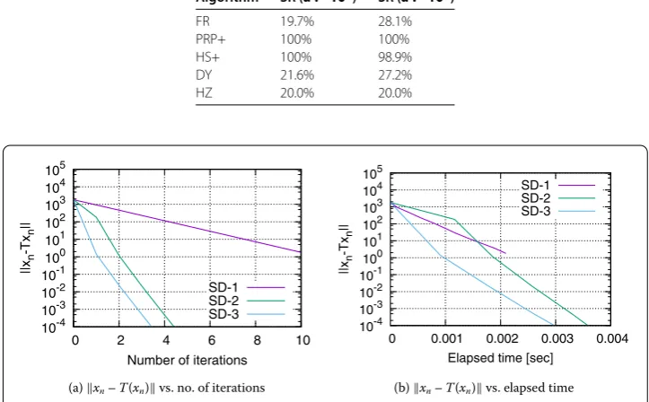
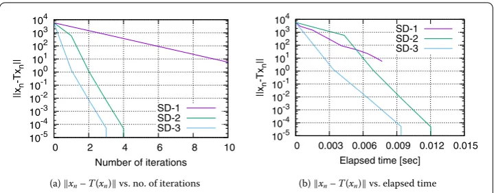
The best conventional nonlinear conjugate gradient method for unconstrained smooth nonconvex optimization was proposed by Hager and Zhang [, ], and it uses the HS formula defined as in (.):
βnHZ:=
dn,yn
yn– dn yn
dn,yn
,∇f(xn+)
=βnHS– yn
dn,yn
∇f(xn+),dn
dn,yn .
Replacing∇f in the above formula with Id –PC(Id –λ∇f) leads to the HZ-type formula for Problem (.):
βnHZ:=βnHS– yn
dn,yn
xn+–PC(xn+–λ∇f(xn+)),dn
dn,yn
, (.)
whereyn:= (xn+–PC(xn+–λ∇f(xn+))) – (xn–PC(xn–λ∇f(xn))) andβnHSis defined by βnHS:=xn+–PC(xn+–λ∇f(xn+)),yn/dn,yn. We tested Algorithm (.) withβn:=βnHZ defined by (.) in order to see how it works on Problem (.).
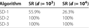
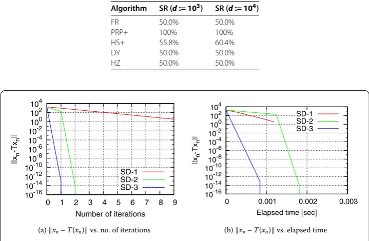
We used the Virtual Desktop PC at the Ikuta campus of Meiji University. The PC has GB of RAM memory, core Intel Xeon . GHz CPU, and a Windows . operating system. The algorithms used in the experiment were written in MATLAB (Rb), and they are summarized as follows.
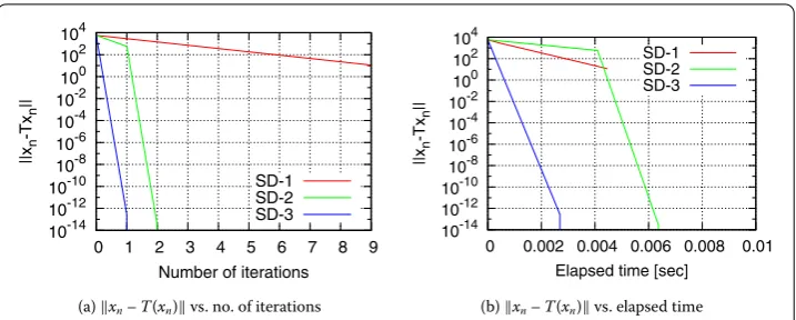
SD-: Algorithm (.) with constant step sizesαn:= .(n∈N) [], Theorem ..
SD-: Algorithm (.) withαnsatisfying the Armijo-type condition (.) whenβ= .
[], Theorems and .
SD-: Algorithm (.) withαnsatisfying the Wolfe-type conditions (.) and (.) and βn:=βnSD(Theorem .).
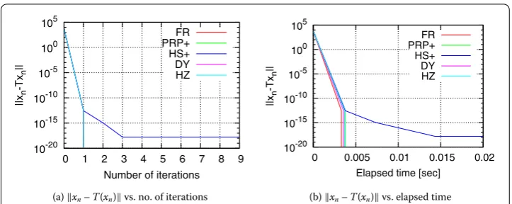
FR: Algorithm (.) withαnsatisfying the Wolfe-type conditions (.) and (.) and βn:=βnFR(Theorem .).
PRP+: Algorithm (.) withαnsatisfying the Wolfe-type conditions (.) and (.) and βn:=βnPRP+(Theorem .).
HS+: Algorithm (.) withαnsatisfying the Wolfe-type conditions (.) and (.) and βn:=βnHS+(Theorem .).
DY: Algorithm (.) withαnsatisfying the Wolfe-type conditions (.) and (.) and βn:=βnDY(Theorem .).
HZ: Algorithm (.) withαnsatisfying the Wolfe-type conditions (.) and (.) and βn:=βnHZdefined by (.) [, ].
The experiment used the following line search algorithm [], Algorithm ., to find step sizes satisfying the Wolfe-type conditions (.) and (.) withδ:= . andσ:= . that were chosen by referring to [], Section ., where, for eachn,An(·) andWn(·) are
An(t): xn(t) –T
xn(t)
–xn–T(xn)
<δtxn–T(xn),dn
,
Wn(t):
xn(t) –T
xn(t)
,dn
>σxn–T(xn),dn