www.adv-radio-sci.net/7/95/2009/
© Author(s) 2009. This work is distributed under the Creative Commons Attribution 3.0 License.
Radio Science
A VLSI design concept for parallel iterative algorithms
C. C. Sun and J. G¨otze
Dortmund University of Technology, Information Processing Lab, Otto-Hahn-Str. 4, 44227 Dortmund, Germany
Abstract. Modern VLSI manufacturing technology has kept shrinking down to the nanoscale level with a very fast trend. Integration with the advanced nano-technology now makes it possible to realize advanced parallel iterative algorithms di-rectly which was almost impossible 10 years ago. In this pa-per, we want to discuss the influences of evolving VLSI tech-nologies for iterative algorithms and present design strate-gies from an algorithmic and architectural point of view. Im-plementing an iterative algorithm on a multiprocessor array, there is a trade-off between the performance/complexity of processors and the load/throughput of interconnects. This is due to the behavior of iterative algorithms. For example, we could simplify the parallel implementation of the iterative al-gorithm (i.e., processor elements of the multiprocessor array) in any way as long as the convergence is guaranteed. How-ever, the modification of the algorithm (processors) usually increases the number of required iterations which also means that the switch activity of interconnects is increasing. As an example we show that a 25×25 full Jacobi EVD array could be realized into one single FPGA device with the simplified µ-rotation CORDIC architecture.
1 Introduction
Modern VLSI manufacturing technology has kept shrinking down to Deep Sub-Micron (DSM) with a very fast trend and Moore’s law is expected to hold for the next 10 years (Gelsinger, 2008). Now, since the DSM nano-technology allows the integration of an ever-increasing number of IP macro-cells on a single silicon die, parallel multiprocessor platforms have received great attention and have been re-alized into several state-of-the-art applications (e.g., Dual-Core CPU, MPSoC and Parallel Computing) (Vangal et al., 2007; Wolf, 2004; Vitullo et al., 2008).
10 years ago, for 0.35µm technology, design engineers were focusing on reducing the area size. Later, when it came
Correspondence to: C. C. Sun
to 0.13µm technology they paid huge efforts to improve the signal delay and reduce the power consumption. As the VLSI manufacturing technology keeps shrinking down into 65 nm, the design methodology for nano-circuits poses new chal-lenges: area requirements of the wire interconnections are increasing explosively in relation to the area of processor el-ements, bus transmission bottleneck in the million transis-tors SoC designs, and leakage current is now dominating the power consumption (Sainarayanan et al., 2007; Stine et al., 2007).
These changes bring us to analyze the impacts on paral-lel iterative algorithms as VLSI technology keeps evolving. As long as the convergence properties of the iterative algo-rithms are guaranteed, it is possible to modify/simplify the architecture during the iteration steps and reduce the com-putational complexity significantly with regard to the imple-mentation. However, this simplification will usually cause an increased number of iterations for convergence. Therefore, it actually becomes a trade-off problem between the perfor-mance/complexity of the hardware, the load/throughput of interconnects and the overall energy/power consumption due to the behavior of parallel iterative algorithms.
Computing the Eigenvalue Decomposition (EVD) with the parallel Jacobi method is used as an example since the con-vergence of this methodology is very robust to modification of the processor elements. Finally, a VLSI design concept for parallel iterative algorithms is presented which takes into ac-count the influence of the modifications on area, timing delay and power consumption.
2 Design concept and implementation issues
A design concept for parallel iterative algorithms, is pre-sented taking into consideration the influences of different VLSI technologies in terms of area, power and timing de-lay. Implementing an iterative algorithm on a multiprocessor array, there is a trade-off between the complexity of an itera-tion step (assuming that the convergence of the algorithm is retained) and the number of required iteration steps. For ex-ample, suppose we have a hardware platform, which requires an iteration step of the iterative algorithm to be executedK times in order to obtain the convergence. The iteration step is executed in parallel on the platform. If we simplify the processors in order to improve the logical utilization of the platform, the number of required iterations usually increase fromK toK+L. It also means that the switch activity of interconnects between these processor elements is increas-ing due to the behavior of iterative algorithm. How to find a superior solution to balance the design criteria is the major issue of this paper, especially for low-power or limited-area devices.
In this paper, we selected the Jacobi EVD method as a typ-ical iterative algorithm since the convergence of this method-ology is very robust to modification of the processor elements (Brent and Luk, 1985; Gotze et al., 1993; Goetze and Hek-stra, 1995; Klauke and Goetze, 2001). We have investigated the influences in DSM design with different sizes of multi-processor arrays (i.e., 4×4, 16×16 and 25×25). After that, several modifications of the algorithm/processor were stud-ied and their impacts on different FPGA devices were inves-tigated (e.g., Xilinx Virtex series in 0.22µm, 0.15µm and 65 nm). According to these analyses, we present an efficient strategy to comply with the design criteria, especially in bal-ancing the number of iterations and the computational com-plexity.
3 Eigenvalue decomposition
An Eigenvalue decomposition of a real symmertric n×n matrix A is obtained by factorizing A into three matrices A=Q∧QT, where Qis an orthogonal matrix (QQT=I) and∧is a diagonal matrix which contains the eigenvalues of A.
3.1 Jacobi method
The cyclic-by-row Jacobi method computes the EVD of a n×nsymmetric matrix iteratively by applying a sequence of orthonormal rotations to the left and the right of the matrix A, as shown in the following:
Ak+1=QkAkQTk, with k=0,1,2, . . . , (1)
whereQk is an orthonormal rotation by the angleθ in the (i, j )plane:
Qk=
col i col j
↓ ↓
1 0 · · · 0
0 . ..
cosθk sinθk ← row i
..
. . .. ...
−sinθk cosθk ← row j
. .. 0
0 · · · 1
.
(2) The order of sequential plan rotations{Qk}is called cyclic-by-row manner, if(i, j )is chosen as follows:
(i, j )=(1,2)(1,3) . . . (1, n)(2,3) . . . (2, n) . . . (n−1, n) . (3) The execution of allN=n(n−1)/2 index pairs(i, j )is called a sweep. After several sweeps are applied, the matrix A will converge into a diagonal matrix∧, which contains the eigen-values:
lim k→∞Ak
= diag[λ1, λ2, . . . , λn] =
λ1 0 · · · 0
0 λ2 ...
..
. . .. 0 0 · · · 0 λn
. (4)
In practice we can observe the Frobenius norm of the off-diagonal elements until it is close to zero or perform a prede-fined number of sweeps which depends on the size of matrix A.
We have to choose the rotation angle in order to annihi-late the off-diagonal elements of Matrix A by solving a 2×2 symmetric EVD subproblem as shown in the following:
a0
ii a
0
ij a0j iajj0
=
cosθ −sinθ sinθ cosθ
aii aij aj i ajj
cosθ −sinθ sinθ cosθ
T
.
(5) We can solve the subproblem and cause the maximal reduc-tion{ai,j, aj,i}=0 by applying an optimal angle of rotation θopt:
θopt=
1
2arctan(τ ) , (6)
whereτ= 2aij
ajj−aii , and the range ofθoptis limited to|θopt|≤
π
a65
a55
a56
a66
a67
a57
a58
a68
a85
a75
a76
a86
a87
a77
a78
a88
P E11 P E13
P E21 P E22
P E14
P E24
P E23
P E44
P E34
P E33
P E31
P E41 P E42 P E43
P E12
P E32
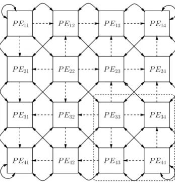
Fig. 1. A 4×4 EVD array,n=8.
3.2 Parallel Jacobi EVD array
The parallel array presented by Brent and Luk consists of n
2×
n
2 Processor Elements (PEs) and each PE contains a 2×2
sub-block of the matrix to be decomposed (Brent and Luk, 1985). Figure 1 shows a typical 4×4 EVD array with 16 PEs. This systolic Jacobi array can perform n2 subproblem in parallel and each sweep requiresn−1 steps. Initially each PE holds a 2×2 sub-matrix ofA:
P Epq =
a2p−1,2q−1a2p−1,2q a2p,2q−1 a2p,2q
,
wherepandq =1,2,· · ·,n2.
(7)
The optimal angel θopt, which is able to annihilate the
off-diagonal elements (a2p−1,2q anda2p,2q−1), is computed
by diagonal PEs (i.e.,P E11,P E22,P E33 andP E44) using
Eq. (6). After these rotation angles are computed, they will be sent to the off-diagonal PEs. This transmission is indi-cated by the dashed lines in Fig. 1. All PEs will perform a two-sided rotation with the corresponding row(θr)and col-umn(θc)rotation angles.
P Epq0 = Q(θr)·P Epq·Q(θc)T,
whereQ(θ )=
cosθ −sinθ sinθ cosθ
. (8)
One sweep needs to performn−1 parallel rotation steps. Af-ter these rotations are applied, the local matrices are inAf-ter- inter-changed between processors as indicated by the solid lines in Fig. 1 for execution of the next sweep. We can use the CORDIC processor to realize the BLV EVD array (Walther, 1971; Volder, 1959; Parhi and Nishitani, 1999). It should be noticed that since we selected the CORDIC processor to ap-proximate the rotation, we can transmit the tanθoptdirectly
instead of the angles (see Sect. 4). In this way, we can
im-prove efficiency of the communication bus and make this sys-tolic array more suitable for VLSI implementation.
4 Architecture considerations
In this section we will show the reasons why it is necessary to simplify the CORDIC architecture and how to achieve this goal. As the evaluation of the VLSI technology keeps shrink-ing down to the nanoscale, it is possible to implement a full Jacobi EVD array into one single FPGA device (Ahmed-said et al., 2003). However if we still use the original full CORDIC processor which is generated by the Xilinx IP-CORE library (www.xilinx.com), only moderate parallelism can be obtained due to the limited FPGA configuration re-sources. For example, we could only realize a 6×6 multicore array at most in the biggest Xilinx FPGA device as shown in Table 2. Therefore, we must simplify the CORDIC architec-ture in order to fit the design criteria.
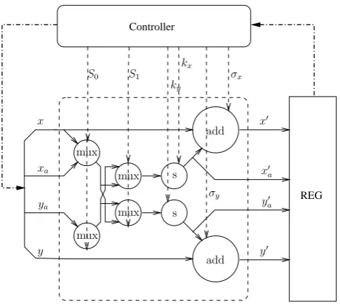
At first we have slightly modified a simplified scaling freeµ-rotation CORDIC which was presented in Goetze and Hekstra (1995) as shown in Fig. 2. It is able to perform the single inner iteration efficiently. This simplified PE has 2 adders, 2 shifters and 4 multiplexers, and it reduces the num-ber of inner iterations from 16 or 32 times for a full CORDIC with word length 16 and 32 bits, respectively, to only one or 6 inner iterations with the CORDIC circular rotation mode. However, decreasing the inner iterations will cause an in-creased number of outer sweeps because of the imprecise inner iterations. Therefore, the simplified CORDIC archi-tecture can reduce the size of area but requires more sweeps. On the other hand, the full CORDIC architecture needs fewer sweeps but requires more area.
Controller
REG
add
add
ya
y
x
a
x
y
a
y xa
x
s
s mux
mux
mux mux
σy
σx
kx
ky
S1 S0
Fig. 2. The block diagram of a simplified CORDIC PE, including 2
adders, 2 shifters and 4 multiplexers.
a given accuracynm, this look-up table is constructed using the aforementioned four approximation methods in Goetze and Hekstra (1995). These orthonormalµ-rotations are cho-sen such that they satisfy a predefined accuracy condition in order to approximate the original rotation angles and are con-structed by the cheapest possible method. It should be no-ticed that we have slightly modified the look-up table. First, since we only need the tanθfor searching the optimal angle in Eq. (6), we can store 2×tanθinstead of performing arctan operation to reverse the rotation angle in the look-up table. Second, we look into the critical path in Table 1. For angle indexk=−1, it requires six cycles per iteration. In fact, the global clock in synchronous circuit is usually determined by the critical path, which also means that the maximum timing delay per iteration is 6 cycles. Therefore, in order to improve the computational balance, we repeat the inner iteration steps of the angles until they are close to the critical one. For ex-ample, when an optimal rotation angle indexk=−8, it will repeat three times from the index−8 to the index−10. In this way, we can balance the overall computing overhead and improve the computational efficiency.
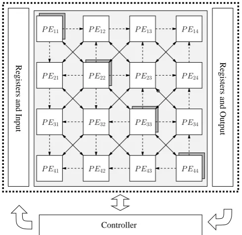
Figure 3 shows a block diagram of a 4×4 full Jacobi EVD array including one controller and 16 PEs. The shaded di-agonal processors will first search the optimal rotation angle and then forward these angles to the off-diagonal PEs.
5 Experimental results
In this work, we have simulated four different cases of the cyclic–by–row parallel Jacobi EVD method in Matlab and on Xilinx FPGA respectively:
Table 1. The setAofµ-rotations for 32-bit accuracy, showing the method used, the tanθangle and the cost of rotation and scaling.
angle index
method angle cost (shift-add operations)
cycle repeat
k 2×tanθk rot. scl. count
−1 IV 1.49070 4 8 6 1
−2 IV 0.54296 4 6 5 1
−3 IV 0.25501 4 6 5 1
−4 IV 0.12561 4 4 4 1
−5 III 6.25841×10⁻² 6 0 3 2 −6 III 3.12606×10⁻² 6 0 3 2 −7 III 1.56263×10⁻² 6 0 3 2
−8 II 7.81266×10⁻³ 4 0 2 3 −9 II 3.90627×10⁻³ 4 0 2 3 −10 II 1.95313×10⁻³ 4 0 2 3
−11 II 9.76563×10⁻⁴ 4 0 2 3
−12 II 4.88281×10⁻⁴ 4 0 2 3
−13 II 2.44141×10⁻⁴ 4 0 2 3 −14 II 1.22070×10⁻⁴ 4 0 2 4 −15 II 6.10352×10⁻⁵ 4 0 2 5
−16 I 3.05176×10⁻⁵ 2 0 1 6 −17 I 1.52588×10⁻⁵ 2 0 1 6 −18 I 7.62939×10⁻⁶ 2 0 1 6 −19 I 3.81470×10⁻⁶ 2 0 1 6 −20 I 1.90735×10⁻⁶ 2 0 1 6 −21 I 9.53674×10⁻⁷ 2 0 1 6 −22 I 4.76837×10⁻⁷ 2 0 1 6 −23 I 2.38419×10⁻⁷ 2 0 1 6
−24 I 1.19209×10⁻⁷ 2 0 1 6 −25 I 5.96046×10⁻⁸ 2 0 1 6 −26 I 2.98023×10⁻⁸ 2 0 1 6 −27 I 1.49012×10⁻⁸ 2 0 1 6 −28 I 7.45058×10⁻⁹ 2 0 1 5 −29 I 3.72529×10⁻⁹ 2 0 1 4 −30 I 1.86265×10⁻⁹ 2 0 1 3 −31 I 9.31323×10⁻¹⁰ 2 0 1 2 −32 I 4.65661×10⁻¹⁰ 2 0 1 1
1. Full rotation CORDIC with 32 iteration steps. 2. Half rotation CORDIC with 16 iteration steps.
3. Simplifiedµ-rotation CORDIC with one single inner it-eration step (µ-CORDIC).
4. Simplified µ-rotation CORDIC with 6 inner iteration steps (6-CORDIC).
5.1 Matlab simulation
Registers and Input Registers and Output
Controller P E13
P E21 P E22
P E14
P E24
P E23
P E44
P E34
P E33
P E31
P E41 P E42 P E43
P E12
P E32
P E11
Fig. 3. The block diagram of a 4×4 Jacobi EVD array with 16µ -rotation elements for FPGA implementation.
also simulated the number of the sweeps as shown in Fig. 5. Here, when the Jacobi EVD array’s size is 20×20, the µ-CORDIC requires 13 sweeps which is almost twice than the Full CORDIC. Although the simplifiedµ-rotation CORDIC PE can improve the computational efficiency, it also in-creases the timing delay. The simplified 6-CORDIC not only requires less sweeps than the µ-CORDIC but also reduces the timing delay. Therefore, the simplified 6-CORDIC is ac-tually a good compromise between the timing delay and the computational effort.
Consequently, from an algorithmic point of view, there is no doubt that we would rather realize the Jacobi method by utilizing the orthonormal simplifiedµ-rotation CORDIC method. However, when it comes to the VLSI circuit design (i.e., here we use VHDL for RTL design), things become to-tally different.
5.2 FPGA implementation
We have modeled a µ-rotation CORDIC PE in VHDL and compared with a full-pipeline CORDIC which is gen-erated by the Xilinx Coregen automatically. Later, we synthesized these two CORDIC processors by Xilinx ISE into three different FPGA devices. It should be noticed that the word-length is 32 bits. Table 2 shows the syn-theses results for Area, Timing Delay and the size of EVD array for each FPGA device (e.g., XCV1000-6FG680 0.22µm, XC2V8000-5FF1517 0.15µm and XC5VL330-2FF1760 65 nm). There are some important points that can be observed.
0 5 10 15 20 25
0 1 2 3 4 5 6 7x 10
6
Size of Jacobi EVD Array
Number of Shitf and Add operations
Full CORDIC 16−rotations One step CORDIC−6
Fig. 4. Number of Shift-Add operations vs. Jacobi EVD array sizes
for different CORDIC solutions.
5 10 15 20 25
0 2 4 6 8 10 12 14 16 18
Size of Jacobi EVD Array
Number of Sweeps
Full CORDIC 16−rotations One step CORDIC−6
Fig. 5. The required number of sweeps vs. Jacobi EVD array sizes
for different CORDIC solutions.
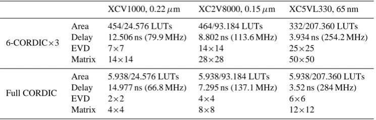
Table 2. Area, Delay and the maximal size of EVD array of different Xilinx FPGA devices (i.e., XCV1000-6FG680, XC2V8000-5FF1517
and XC5VL330-2FF1760).
XCV1000, 0.22µm XC2V8000, 0.15µm XC5VL330, 65 nm
6-CORDIC×3
Area 454/24.576 LUTs 464/93.184 LUTs 332/207.360 LUTs Delay 12.506 ns (79.9 MHz) 8.802 ns (113.6 MHz) 3.934 ns (254.2 MHz)
EVD 7×7 14×14 25×25
Matrix 14×14 28×28 50×50
Full CORDIC
Area 5.938/24.576 LUTs 5.938/93.184 LUTs 5.938/207.360 LUTs Delay 14.977 ns (66.8 MHz) 7.295 ns (137.1 MHz) 3.52 ns (284 MHz)
EVD 2×2 4×4 6×6
Matrix 4×4 8×8 12×12
matrix size of the full CORDIC. Therefore, utilizing the Full CORDIC would cause a partition problem and the processor array would require handling the partition sequentially. This requires an external memory and a more complicated control routine.
6 Conclusions
In this paper, we presented a design concept for parallel iterative algorithms when the VLSI design keeps evolving into nanoscale. For iterative algorithms we are able to sim-plify/modify the PEs as long as the convergence is guaran-teed, such that the parallelism of the implementation can be increased. This is paid for by an increased number of it-erations. Computing the EVD by the parallel Jacobi algo-rithm was used as an example. We have synthesized it into three different Xilinx FPGA devices. The experimental re-sults show that we can realize a 25×25 full Jacobi EVD ar-ray into Xilinx XC5VL330 65nm FPGA device. In future work we will investigate the influences of the interconnects, i.e., with advancing VLSI technology the simplified PEs be-come smaller and smaller in comparison with the intercon-nection structure of the processor array. This fact requires that the varying importance of interconnects must be incor-porated into the design concept.
References
Ahmedsaid, A., Amira, A., and Bouridane, A.: Improved SVD sys-tolic array and implementation on FPGA, in: IEEE International Conference on Field-Programmable Technology (FPT), pp. 3– 42, 2003.
Brent, R. P. and Luk, F. T.: The Solution of Singular-Value and Symmetric Eigenvalue Problems on Multiprocessor Arrays, SIAM Journal on Scientific and Statistical Computing, 6, 69–84, 1985.
Gelsinger, P.: Moore’s Law: “We See No End in Sight,”, Tech. rep., Intel Chief Technology Officer, http://websphere.sys-con. com/node/557154, 2008.
Goetze, J. and Hekstra, G.: An Algorithm and Architecture Based on Orthonormal Micro-Rotations for Computing the Symmetric EVD, INTEGRATION – The VLSI Journal, 20, 21–39, 1995. Gotze, J., Paul, S., and Sauer, M.: An Efficient Jacobi-Like
Algo-rithm for Parallel Eigenvalue Computation, IEEE Transactions on Computers, 42, 1058–1065, 1993.
Klauke, S. and Goetze, J.: Low Power Enhancements for Parallel Algorithms, in: IEEE International Symopsium on Circuits and Systems, 2001.
Parhi, K. K. and Nishitani, T.: Digial Signal Processing for Multi-media Systems, MARCEL DEKKER, New York, 1999. Sainarayanan, K. S., Raghunandan, C., and Srinivas, M.: Delay
and Power Minimization in VLSI Interconnects with Spatio-Temporal Bus-Encoding Scheme, in: IEEE Computer Society Annual Symposium on VLSI, pp. 401–408, 2007.
Stine, J. E., Castellanos, I., Wood, M., Henson, J., Love, F., Davis, W. R., Franzon, P. D., Bucher, M., and Basavarajaiah, S.: FreePDK: An Open-Source Variation-Aware Design Kit, in: IEEE International Conference on Microelectronic Systems Ed-ucation, pp. 173–174, 2007.
Vangal, S., Howard, J., Ruhl, G., Dighe, S., Wilson, H., Tschanz, J., Finan, D., Iyer, P., Singh, A., Jacob, T., Jain, S., Venkatara-man, S., Hoskote, Y., and Borkar, N.: An 80-Tile 1.28TFLOPS Network-on-Chip in 65 nm CMOS, Solid-State Circuits Confer-ence, 2007. ISSCC 2007. Digest of Technical Papers. IEEE In-ternational, pp. 98–589, 2007.
Vitullo, F., L’Insalata, N. E., Petri, E., Saponara, S., Fanucci, L., Casula, M., Locatelli, R., and Coppola, M.: Low-Complexity Link Microarchitecture for Mesochronous Communication in Networks-on-Chip, IEEE Transactions on Computer, 57, 1196– 1201, 2008.
Volder, J.: The CORDIC trigonometric computing technique, IRE Trans. Electron. Comput., EC-8, 330–334, 1959.
Walther, J.: A unified algorithm for elementary functions, in: Proc. Spring Joint Comput. Conf., vol. 38, pp. 379–385, 1971. Wolf, W.: The future of multiprocessor systems-on-chips, in: