c
Copernicus GmbH 2003
Advances in
Radio Science
Speaker tracking with a microphone array using Kalman filtering
D. Bechler, M. Grimm, and K. Kroschel
Institut f¨ur Nachrichtentechnik, Universit¨at Karlsruhe, Kaiserstr. 12, 76128 Karlsruhe, Germany
Abstract. In this publication a method for tracking a speaker
with acoustical information by means of a microphone array is presented. A sound source localization algorithm based on the time delays of arrival of sound waves in microphone pairs provides initial position estimates. These significantly varying estimates are spatially filtered by an adaptive Kalman filter to obtain a smoothed trajectory of the speaker’s move-ment. Experimental results with real data are presented for a variety of scenarios recorded in a noisy and reverberant of-fice room environment.
1 Introduction
Integrating acoustic perception by means of a microphone ar-ray into autonomous humanoid robots is nowadays an impor-tant area of research. The aim of the robot’s hearing system is not only to be able to interact with a human operator but also to create an acoustic map of the sound environment and to perform an acoustic scene analysis, i.e. the localization, separation and classification of sound sources present in the acoustic environment. Especially the task of acoustically lo-calizing a speaker in a room environment is of great interest not only in robotics but also for teleconferencing or acoustic surveillance systems.
The technique of choice in most recent acoustic localiza-tion systems using microphone arrays is a two-step proce-dure. First, the time delay of arrival (TDOA) of sound signals in a pair of spatially separated microphones is estimated. In a second step the estimated TDOAs of different microphone pairs are used in combination with the microphone array ge-ometry to localize the sound source. To avoid the compu-tational demanding solution of a set of non-linear equations for the exact sound source position, sub-optimal closed-form localization estimators with satisfactory precision can be ap-plied (DiBiase et al., 2001; Huang et al., 2000).
Correspondence to: D. Bechler
Due to the one-sample-precision of the TDOA estimation algorithm and due to noise and reverberation influences, the TDOA estimates and the real TDOA values are not identi-cal which leads to relatively high variances in consecutive position estimates. In this publication a method to smooth the speaker trajectory and to assure robustness by means of an adaptive Kalman filter is evaluated for a real data single speaker scenario in a noisy and reverberant office environ-ment.
The paper is organized as follows: In Sect. 2 the localiza-tion of sound sources based on time delay estimates is pre-sented. Filtering the initial estimates of the sound source po-sition by an adaptive Kalman filter is discussed in Sect. 3. Section 4 describes the experimental setup. In Sect. 5 we present and evaluate the obtained results. Finally, some con-clusions are drawn and an outlook for future work is given.
2 Time- delay- based localization of sound sources
2.1 Signal model
For a given pair of spatially separated microphonesMi and Mj, the recorded sensor signalsxi(t )andxj(t )for a signal s(t ), emanated from a remote sound source in a reverberant and noisy environment, can be modeled mathematically as
xi(t )=hi(t )∗s(t )+ni(t )
2.2 TDOA estimation with GCC method
The most popular approach for determining the TDOAs is called the Generalized Cross-Correlation (GCC) method Knapp and Carter (1976). The relative time delayτij is esti-mated as the time lag with the global maximum peak in the GCC functionRij(g)(τ )
ˆ τij =
argmax τ R
(g)
ij (τ ). (2)
This GCC functionR(g)ij (τ )is defined as
Rij(g)(τ )= Z +∞
−∞
ψij(ω)Xi(ω)Xj(ω)∗ej ωτdω. (3) The weighting function ψij(ω) intends to decrease noise and reverberation influences and tries to emphasize the GCC value at the true TDOA valueτij. For real environments the Phase Transform (PHAT) technique (Knapp and Carter, 1976) has shown the best performance. This PHAT weight-ing function is defined as
ψijP H AT(ω)= 1 |Xi(ω)Xj(ω)∗|
. (4)
2.3 Confidence criteria for TDOA estimates
To detect outliers in TDOA estimates, two confidence crite-ria can be used: the value of the maximum peak and the ratio between the 1stand the 2ndpeak in the GCC function (Bech-ler and Kroschel, 2002a,b). These criteria allow a reliability scoring of individual estimates and can be used to reject er-roneous measurements. The higher the value of these prop-erties of the GCC function the higher the probability that the TDOA was estimated correctly.
2.4 Data association and clustering of TDOA estimates With the confidence criteria described in Sect. 2.3, a tradeoff has to be made between a high number of estimates neces-sary for a continuous source tracking, and a high percentage of correct TDOA estimates, which is crucial for robust source localization. Additionally, the one-sample-precision of the GCC algorithm can be too imprecise, which is problematic for the localization algorithm. As a solution we propose data association and clustering techniques for the TDOA es-timates. To initialize an acoustic track, a high reliability is demanded and therefore a high threshold for the value of the confidence criteria is used. Once initialized, this decision threshold can be lowered, as now it is possible to search in a region of interest around the initial TDOA estimate value. Thus, erroneous estimates outside this region of interest can be rejected. In addition, several consecutive TDOA estimates are averaged, which solves the problem of the one-sample-precision. With these data association and clustering tech-niques, the TDOA estimates become sufficiently accurate for the following localization algorithm to produce robust sound position estimates.
2.5 Localization algorithm
To derive from the TDOAs and the microphone array geom-etry the source position, the exact localization necessitates solving a set of non-linear equations, which can be compu-tationally demanding. To accelerate the sound source posi-tion determinaposi-tion, the One-Step Least-Squares (OSLS) al-gorithm (Huang et al., 2000) is used. This closed-form lo-cation estimator approximates precisely enough accurate the exact solution to the non-linear problem.
3 Spatial filtering
For a continuous source trajectory these initial, significantly varying position estimates obtained by the localization al-gorithm described in Sect. 2 are spatially smoothed by a Kalman Filter (KF) as post-processing unit.
3.1 Kalman filtering
For the motion of a speaker the time-discrete state space de-scription by means of a state and an observation equation is used. The state equation is defined as
x(k)=Ax(k−1)+Bu(k) (5) wherex(k)is a state vector at time instantkcontaining the position, the velocity and the acceleration of the sound source in Cartesian coordinates. The time-invariant state transition matrix A as well as the varianceσU2 of the white noiseu(k) representing the system error are assumed to be known. B is the time-invariant system noise coupling matrix mapping the system error to the elements of the state vectorx(k). In the observation equation
y(k)=Cx(k)+n(k) (6)
y(k) is the observation vector containing the source posi-tion, C is the time-invariant measurement matrix mapping the state of the system to the observation vector andn(k)is white noise with the covariance matrix RN N(k)representing the measurement error. For our scenario, in which a speaker can move arbitrarily in the acoustical environment, three mo-tion models are reasonable: a static, a constant velocity and a constant acceleration model (for the definitions of the ac-cording matrices A, B and C cf. Grimm, 2001).
3.2 Filter algorithm
One cycle of the KF is done with the following filter algo-rithm. For a detailed derivation cf. Brown (1983).
In a first step, the updated estimation error covariance ma-trix REE(k+1|k+1)can be derived from the previous co-variance matrix REE(k|k). Therefore, the a priori estimation error covariance matrix REE(k+1|k)at the(k+1)t hiteration givenkobservations is calculated with
With Eq. (7), the covariance matrix Rνν(k+1)of the innova-tionν(k+1)can be calculated, whereν(k)is defined as the difference between the actual observation vectory(k)and the estimated observation vector at thekt hiteration givenk−1 observationsyˆ(k|k−1):
ν(k)=y(k)−yˆ(k|k−1). (8)
Rνν(k+1)is given by
Rνν(k+1)=CREE(k+1|k)CT +RN N(k). (9) The a posteriori estimation error covariance matrix REE(k+ 1|k+1)is then found from
REE(k+1|k+1)=REE(k+1|k) −W(k+1)Rνν(k+1)WT(k+1),
(10) where W(k+1)is the filter gain at instantk+1 defined as
W(k+1)=REE(k+1|k)CT(Rνν(k+1))−1. (11) Similarly, the estimate of the system state can be itera-tively derived from the previous estimate. First, the a priori system state estimate
ˆ
x(k+1|k)=Axˆ(k|k) (12) is calculated and out of it the source position is estimated with
ˆ
y(k+1|k)=Cxˆ(k+1|k). (13) By means of innovation and filter gain the actual state esti-mation results from
ˆ
x(k+1|k+1)=xˆ(k+1|k)+W(k+1)ν(k+1) (14) and the updated source position is found from
ˆ
y(k+1|k+1)=Cxˆ(k+1|k+1). (15) 3.3 Adaptive Kalman Filter
Up to now the different motion model approaches were re-garded independently. As the motion dynamics of a speaker in an office environment are variable, a single model for the KF is not suitable for all situations. Thus, a multiple model system would be advantageous. By means of the definition of a model probability described in this section, several mod-els are used simultaneously for the determination of the final position estimate.
3.3.1 Model probability
ForLmodelsαi with 1 ≤ i ≤ Lthe conditional probabil-ityf (αi|y(k))is the probability that theit hmodel based on the measurements y(1),· · ·,y(k) is the one describing the speaker’s movement correctly. With the Bayes formula we get
f (αi|y(k))=
f (y(k)|αi) f (αi)
f (y(k)) . (16)
KF
a
1KF
a
2KF
a
3C
1C
2C
3y
(k)
x
1(k|k)
^
x
2(k|k)
^
x
3(k|k)
^
y
1(k|k)
^
y
2(k|k)
^
y
3(k|k)
^
y
(k|k)
^
f( | (k))
a
1y
f( | (k))
a
2y
f( | (k))
a
3y
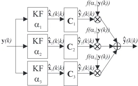
Fig. 1. Block diagram of the adaptive Kalman filter
For this conditional probability a recursive formula can be given:
f (αi|y(k))=
f (y(k)|y(k−1), αi) f (αi|y(k−1)) PL
j=1f y(k)|y(k−1), αjf αj|y(k−1)
. (17) The termsf (y(k)|y(k−1), αi)can be calculated in every recursive step with
f (y(k)|y(k−1), αi)= 1 (2π )32
√ |Rνν,i(k)|
·expn−1
2νiT(k)R
−1
νν,i(k)νi(k) o
.
(18)
3.3.2 Multiple Model Adaptive Estimator (MMAE) The approach using several models for the final estimate si-multaneously is called adaptive KF or Multiple Model Adap-tive Estimator (MMAE) (Bar-Shalom, 1988). In Fig. 1 the block diagram of our adaptive KF is shown. The measure-menty(k)is used in three KFs in parallel to determine one estimate of the system statexˆ1(k|k),xˆ2(k|k)andxˆ3(k|k)for
every of the three models. As mentioned, we use a static, a constant velocity and a constant acceleration model to de-scribe the motion of a speaker. By means of the observa-tion matrices C1,C2 and C3 the system state estimates are
mapped to the observation estimates yˆ1(k|k),yˆ2(k|k) and
ˆ
y3(k|k). These position estimates are weighted with the
corresponding model probabilitiesf (αi|y(k)) according to (Eq. 17) with 1≤i≤ 3 and finally summed up. Hence, the actual position estimate for the adaptive KF is determined with
ˆ
yMMAE(k|k)=
3
X
i=1
f (αi|y(k)Cixˆi(k|k). (19)
4 Experimental setup
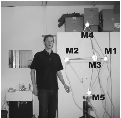
Fig. 2. Experimental setup
data recording we used a 5-microphone array in an equi-lateral double-tetrahedron geometry with a side length of D=28 cm as shown in Fig. 2. 25 scenarios were recorded in which a speaker is uttering German sentences. In addition to stationary positions for a sitting or standing speaker, motions along given trajectories with constant velocity and transitions from stationary positions to constant walking were studied. The sampling frequency wasfs=16 kHz. The recorded data were analyzed in frames of 32 ms to assure quasi-stationarity. For this data segmentation, a Hamming window with a 50% overlap was applied. For the data association and clustering techniques described in Sect. 2.4, the average of the TDOA estimates in a block out of 12 consecutive frames is calcu-lated where blocks are overlapped by 50%. This generates a new position estimate for the sound source every 96 ms. With this averaging, robust speaker tracking is still possible since at least four estimates per second are required (Silver-man and Kirt(Silver-man, 1992) for a moving speaker.
5 Results
The proposed system shows robust speaker localization capa-bilities in a noisy and reverberant environment. The adaptive KF performs its task as post-processing unit in guaranteeing a smoothed continuous trajectory compared with the initial position estimates.
Exemplarily, Fig. 3 shows a comparison of the localization of a stationary speaker at the spherical coordinatesazimut h =95◦,elevat ion= −7.9◦andrange=1.5 m before and after Kalman filtering. The temporal runs of all spherical co-ordinates are significantly smoothed. Note that the variance in range is reduced, but the overall range error increases by applying a KF in this case. Until 1.2 s the localization
algo-0 0.5 1 1.5 2 2.5 3 90
100 110
azimuth [degree]
time [s]
0 0.5 1 1.5 2 2.5 3 −20
−10 0 10
elevation [degree]
0 0.5 1 1.5 2 2.5 3 0.5
1 1.5
range [m] initial position estimatesafter Kalman filtering
Fig. 3. Stationary speaker atazimut h=95◦,elevat ion= −7.9◦ andrange=1.5 m
−1 0
1 2
−0.5 0 0.5 1 1.5 2 −1 −0.5 0 0.5 1
x [m] y [m]
z [m]
Micros Start/Stop Raw data Kalman
Fig. 4. Speaker moving from Cartesian coordinates
(−1m,1m,0.13m)to(1m,1m,0.13m)
rithm underestimates the range by about 50 cm and the KF evidently cannot remedy this systematic error.
An example for tracking a speaker uttering a Ger-man sentence while moving with constant velocity from (−1 m,1 m,0.13 m) to (1 m,1 m,0.13 m) is presented in Fig. 4. In this 3D-plot the true trajectory (arrow) and the positional estimates before and after applying the adaptive KF for a walking speaker are shown. Also in this example the KF functions reliably and delivers a smoothed speaker trajectory. As for this scenario there is no systematic error in the initial position estimates the overall error in all coordinates is re-duced.
6 Conclusions and outlook
jus-tify the complexity of our adaptive Kalman filter as post-processing unit. But the reduction of the overall error of position estimates with an adaptive KF highly depends on the quality of the initial estimates used as KF input. If these estimates show low systematic errors, the KF delivers an ef-ficient smoothing of the initial trajectory. Even if there are erroneous TDOA estimates in only one of the 4 microphone pairs, this can lead to wrong initial position estimates by the localization algorithm, which renders the operation of the filter unreliable. Therefore future work will be devoted to the improvement of the TDOA reliability by considering psychoacoustics, e.g. the precedence effect (Litovsky et al., 1999) to suppress reverberation influences. An additional ad-vantage of the KF lies in its ability to predict source positions in case of missing current position estimates due to speech pauses or non-reliable TDOA estimates.
In this work only one speaker was present in the acoustic scene. Current investigations are concerned with the simulta-neous tracking of multiple active sound sources requiring an according number of KFs working in parallel. Furthermore, it is aimed to extend this tracking system by cameras. With the fusion of acoustic and visual data strong improvements should be achieved compared with a pure acoustic tracker.
Acknowledgements. This work is part of the
Sonderforschungs-bereich (SFB) No. 588 “Humanoide Roboter - Lernende und
kooperierende multimodale Roboter” at the University of
Karls-ruhe. The SFB is supported by the Deutsche Forschungsgemein-schaft (DFG).
References
Bechler, D. and Kroschel, K.: Confidence scoring of time differ-ence of arrival estimation for speaker localization with micro-phone arrays, 13. Konferenz Elektronische Sprachsignalverar-beitung ESSV, September 2002a.
Bechler, D. and Kroschel, K.: Reliability measurement of time dif-ference of arrival estimations for multiple sound source localiza-tion, 17th Annual Meeting of the IAR, November 2002b. Brown, R. G.: Introduction to Random Signal Analysis and Kalman
Filtering, Wiley, 1983.
Bar-Shalom Y.: Tracking and data association, Academic Press, 1988.
DiBiase, J. H., Silverman, H. F., and Brandstein, M. S.: Mi-crophone Arrays, chapter Robust Localization in Reverberant Rooms, Springer, 2001.
Grimm, M.: Passives Audio-Tracking sich bewegender Ger¨auschquellen, Studienarbeit, Institut f¨ur Nachrichtentechnik, Universit¨at Karlsruhe, 2001.
Huang, Y., Benesty, J., and Elko G. W.: Passive acoustic source lo-calization for video camera steering, IEEE Int. Conf. Acoustics, Speech and Signal Processing (ICASSP), 909–912, June 2000. Knapp, C. H. and Carter, G. C.: The generalized correlation method
for estimation of time delay, IEEE Trans. on Acoustics, Speech and Signal Processing, 24(4):320–327, August 1976.
Litovsky, R. Y., Colburn, H. S., Yost, W. A., and Guzman, S. J.: The precedence effect, Journal of the Acoustical Society of America, 106(4):1633–1654, October 1999.