EXTENDING THE PAGE SEGMENTATION ALGORITHMS OF THE OCROPUS DOCUMENTATION LAYOUT ANALYSIS SYSTEM

(1)

by

Amy Alison Winder

A thesis

submitted in partial fulfillment of the requirements for the degree of Master of Science in Computer Science

Boise State University

(2)

(3)

DEFENSE COMMITTEE AND FINAL READING APPROVALS

of the thesis submitted by

Amy Alison Winder

Thesis Title: Extending the Page Segmentation Algorithms of the OCRopus Document Layout Analysis System

Date of Final Oral Examination: 28 June 2010

The following individuals read and discussed the thesis submitted by student Amy Alison Winder, and they evaluated her presentation and response to questions during the final oral examination. They found that the student passed the final oral examination.

Elisa Barney Smith, Ph.D. Co-Chair, Supervisory Committee Timothy Andersen, Ph.D. Co-Chair, Supervisory Committee Amit Jain, Ph.D. Member, Supervisory Committee

(4)

Dedicated to my parents, Mary and Robert, and to my children, Samantha and Thomas.

(5)

The author wishes to express gratitude to Dr. Barney Smith for providing a structured and supportive environment in which to formulate, develop, and complete this thesis. Not only did she provide the initial concept for the work, but she was instrumental in selecting the specific topic and followed through by meeting with me weekly to guide and support this effort. The author is also grateful for the instruction Dr. Barney Smith provided in Image Processing, which, paired with computer science, is an exciting field.

Thanks also go to Dr. Andersen for introducing me to the intriguing world of Artificial Intelligence and for allowing me to fulfill the requirements of my thesis under his advisement. The author is grateful for his contributions to the understanding of page segmentation algorithms and performance metrics.

Additionally, the author appreciates the help of Dr. Jain who has been a reliable source of information for the author’s entire graduate career at Boise State University. Not only did he streamline the author’s academic schedule upon arrival, but he expressed interest and placed value upon the experience and education the author brought to the university, subsequently strengthening her resolve to obtain a second Master of Science degree.

Finally, the author would like to thank the undergraduate students from the university who created and scanned a majority of the document images: Josh Johnson, Kris Burch, and Will Grover.

(6)

of this degree, and a stipend was provided by the United States Government under the Trade Adjustment Assistance Act as petitioned by Micron Technology, Inc., the author’s former employer. The author is grateful for the guidance provided by Ruby Rangel, Senior Consultant at the Idaho Department of Commerce and Labor.

(7)

The author was born in Princeton, NJ and attended Westtown School in Penn-sylvania and the University of Rochester in New York where she earned Bachelor of Science and Master of Science degrees in Optics. Following graduation, she worked in the Electro-Optics Division of Honeywell in the Boston area of Massachusetts, supporting the Strategic Defense Initiative. In the Systems Engineering group, she supported simulation efforts of an infrared sensor and in the Optics group she analyzed telescope lens designs.

After a brief sojourn to raise her children, the author took an engineering position at Micron Technology, Inc. in Boise, Idaho. For five years, she worked in the Advanced Reticle group, supporting the development of new reticles used in the photo-lithography process of semiconductor manufacturing. Then, she transferred to the Design department within which she relocated to Japan as a CAD engineer to support the recently opened DRAM design center. Upon returning to the United States two years later, she designed layouts, wrote Design Rule Verification tool sets, and provided general CAD support until deciding to broaden her skill set by pursuing a Master of Science degree in Computer Science at Boise State University.

(8)

ABSTRACT

With the advent of more powerful personal computers, inexpensive memory, and digital cameras, curators around the world are working towards preserving historical documents on computers. Since many of the organizations for which they work have limited funds, there is world-wide interest in a low-cost solution to obtaining these digital records in a computer-readable form. An open source layout analysis system called OCRopus is being developed for such a purpose. In its original state, though, it could not process documents that contained information other than text. Segmenting the page into regions of text and non-text areas is the first step of analyzing a mixed-content document, but it did not exist in OCRopus. Therefore, the goal of this thesis was to add this capability so that OCRopus could process a full spectrum of documents.

By default, the RAST page segmentation algorithm processed text-only docu-ments at a target resolution of 300 DPI. In a separate module, the Voronoi algorithm divided the page into regions, but did not classify them as text or non-text. Addition-ally, it tended to oversegment non-text regions and was tuned to a resolution of 300 DPI. Therefore, the RAST algorithm was improved to recognize non-text regions and the Voronoi algorithm was extended to classify text and non-text regions and merge non-text regions appropriately. Finally, both algorithms were modified to perform at a range of resolutions.

Testing on a set of documents consisting of different types showed an improvement of 15-40% for the RAST algorithm, giving it at an average segmentation accuracy

(9)

70% overall. Depending on the layout of the historical documents to be digitized, though, either algorithm could be sufficiently accurate to be utilized.

(10)

LIST OF FIGURES

2.1 Example of RAST output of OCRopus. Note the multiple colors in both figures. . . 18 2.2 Example of RAST output of OCRopus. Note the text coloring of the

x-axis labels and the absence of the y-axis labels. . . 19 2.3 Example of RAST output of OCRopus. Note the column dividers in

the table and the absence of some entries. . . 21 2.4 Example of Voronoi output of OCRopus. Note the oversegmentation

of the figures. . . 23 2.5 Example of Voronoi output of OCRopus. Note the oversegmentation

of the graphs. . . 24 2.6 Example of Voronoi output of OCRopus. Note the oversegmentation

of the table. . . 25

3.1 XML file data structure. . . 29 3.2 Example of Match Score tables - actual value on the left, thresholded

on the right - and G and D-profiles. Taken from page 851 of [24]. . . 30 3.3 This figure illustrates character boxes that were not overlapped by any

text line boxes and had been previously omitted from consideration as either text or graphics. . . 35 3.4 This figure illustrates small isolated character boxes that had been

(15)

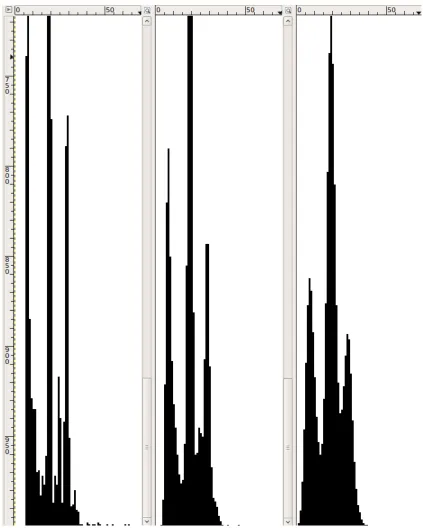
that it fully encloses the figure. . . 38 3.7 Histogram of the heights of the bounding boxes of the connected

com-ponents with no smoothing (left), one iteration of smoothing (middle) and two iterations of smoothing (right). The rightmost peak corre-sponds to the height of ascenders (i.e. tall letters), the middle peak to the height of x-height characters (i.e. short letters) and the leftmost to the height of periods, commas, etc. . . 40 3.8 Steps of the improved RAST algorithm. The original steps have a

standard font, the modified functions are italicized and new functions are bold. . . 41 3.9 The numbered Vornonoi zones. The histograms in Figures 3.12-3.14

correspond to tan text zone number #8. . . 43 3.10 The Vornonoi lines. . . 44 3.11 The ”text rectangle” of an unclassified zone. . . 45 3.12 Section of the histogram of the y0-values of the character boxes of zone

#8 in Figure 3.9. The peaks to the left correspond to letters extending below the line and the peaks to the right correspond to letters sitting on the line. . . 46 3.13 Section of the smoothed histogram of Figure 3.12. . . 46 3.14 Histogram of the peaks of the y0-values of the histogram of Figure 3.13.

In this example, for each of the lines, the median number of occurrences of the main y0-value is twelve. . . 47

(16)

3.15 Zone coloring of non-text relabeling process. a) Initial zone coloring, b) after the smallest has been relabeled, c) after its neighbor has been relabeled and d) after all of the neighboring non-text zones have been

relabeled. . . 48

3.16 Pictures in two different columns are merged. . . 50

3.17 Merged graphics zone is broken in two and text overlaps removed. . . 51

3.18 Wrap around text zone covers picture. . . 52

3.19 Wrap around text zone is broken into two zones. . . 52

3.20 Steps of the extended Voronoi algorithm. The original steps have a standard font and the new functions are bold. . . 53

4.1 Performance of original (top) and improved (bottom) RAST algorithms with the ICDAR Page Segmentation Competition weights (left) and the weights compensated for segmentation of paragraphs (right). Higher numbers indicate higher performance. . . 57

4.2 Example of text oversegmentation in the improved RAST algorithm. Note the line in the middle of the left column that has been defined as one region. It is slightly longer than the line above and below it. . . 60

4.3 Example of column merging in the improved RAST algorithm. Note the diminutive height of the merged columns at the bottom of the page. 61 4.4 Example of text-image merging in the improved RAST algorithm. Note the ”Ich” word to the left of the upper figure separated from the rest of the text on the line with -:””. . . 63

(17)

weights (left) and the weights compensated for segmentation of para-graphs (right). . . 64 4.6 Ground truth of a single text-only document image. . . 66 4.7 Voronoi text segments of a single text-only document image. . . 67 4.8 Voronoi segmentation of a mixed column document with pictures at

300 DPI. The lowest regions were classified as graphics. The accuracy of the segmentation was 37%. . . 69 4.9 Voronoi segmentation of a mixed column document with pictures at 600

DPI. Most of the lowest regions were classified as text. The accuracy of the segmentation was 53%. . . 70 4.10 Document image where the picture is placed too close to the text to

allow for correct Voronoi zoning. Note the purple text section merged with the rabbit. . . 71 4.11 Fine Reader text segments of a single text-only document image. . . 74 4.12 Performance of ABBYY’s Fine Reader Engine 9.0 (bottom), the

ex-tended Voronoi algorithm (middle) and the improved (top) RAST algorithm. . . 75 4.13 Example of Fine Reader segmentation. Note the overlapping image

and text boxes. . . 76

(18)

LIST OF ABBREVIATIONS

DRAM – Dynamic Random Access Memory

CAD – Computer Aided Design

CCD– Charge-Coupled Device

PDF – Portable Document Format

OCR – Optical Character Recognition

MP – Mega Pixel

DPI – Dots Per Inch

IUPR – Image Understanding Pattern Recognition

ASCII– American Standard Code for Information Interchange

RXYC – Recursive X-Y Cut

RLSA– Run-Length Smearing Algorithm

DAFS – Document Attribute Format Specification

XML– eXtensible Markup Language

PSET – Page Segmentation Evaluation Toolkit

ICDAR – International Conference on Document Analysis and Recognition

HTML – Hyper Text Markup Language

CSS – Cascading Style Sheets

(19)

SAX – Simple API for XML

DOM – Document Object Model

(20)

1

CHAPTER 1 INTRODUCTION

The ability to create, store, and modify documents on computers has only existed for two to three decades. The printing press, on the other hand, invented in Germany and adopted by the rest of the developed world over time, has been in use for nearly six centuries [1]. Consequently, a multitude of printed documents have been generated in book, magazine, and newspaper form. While many have been lost over the years, a significant portion has been preserved. As historical documents, they are not only fragile, but are inaccessible to most people. In the interest of sharing and preserving their contents for eternity, there is a movement to digitize and store them on computers.

At this time, the most common method for digitizing documents is to use an image scanner [3]. Image scanners, also known as flatbed or desktop scanners, contain a light source, an image sensor such as a CCD, and a glass top upon which the document is placed. Standard scanners that scan documents and produce images of them cost a few hundred dollars; however, it is also possible to purchase large format scanners capable of scanning large books and converting the images into searchable PDF files, but they cost on the order of five thousand dollars. In standard scanners, documents are digitized by OCR software installed onto the computer.

(21)

the pages of books, the bindings of which may be too brittle to withstand the pressure of being placed, and temporarily deformed, on a scanner bed. Once these images have been obtained, it is necessary to process and analyze them so that they can be converted into text documents that are easily readable and searchable. Since the institutions that house many of these documents have limited funds, a low-cost solution to digitization is the only feasible option.

The impetus for this thesis was a non-profit organization in Germany called the Bavarian Traditional Clothing Culture Center and Archive [2], which was formed to preserve traditional Bavarian costumes and dances. It has been acquiring the newspapers and magazines of various clubs in the area, which it plans to house in a new archive facility. The organization then hopes to digitize these documents so that researchers can examine them to gain a better understanding of how costumes and dance have evolved over the years. Many of these documents were written in the German Fraktur font and contain illustrations, but have standard Manhattan layouts.

(22)

3

1.1 Document Recognition and Analysis

1.1.1 Image Acquisition and Processing

The first step in the process of digitizing a document is to capture an image of it. This can be done by either scanning or photographing it. Mid-priced digital cameras are capable of taking pictures with resolutions of 3,872 x 2,592 pixels (10 MP) to 4,672 x 3,104 pixels (15 MP). When these images are printed out at a resolution of 300 DPI, they range in size from 12.9” x 8.6” to 15.6” x 10.3”, approximately the same size as a page of a bound historical document. Typical desktop scanners can image documents with resolutions of 150 to 1200 DPI. So, today’s common digital cameras can produce images comparable to those generated by a desktop scanner.

Employing digital cameras for image acquisition, on the other hand, introduces a host of other issues that need to be resolved before the documents can be analyzed. First, unless the camera is lined up perfectly with the page, it can capture some areas outside of it including the table top, the adjacent page, and the edges of the pages residing between it and the outer cover. The extraneous information contained within these areas generally needs to be removed prior to analyzing the document so that only the relevant sections of the document are analyzed. This process is typically referred to as border removal.

(23)

This is called binarization. Additionally, if there is speckle noise present on the page, it will need to be removed as well.

At this time, there is an open source program called PhotoDoc [5] that is capable of handling all of these issues except for noise removal and distortion caused by warping. PhotoDoc can be used in conjunction with an OCR engine such as (open source) Tesseract [6] or OCRopus for image-to-text conversion. In addition to PhotoDoc, researchers in the Image Understanding Pattern Recognition (IUPR) Research Group of Kaiserslautern, Germany, in partnership with the Adaptive Technology Resource Centre of Toronto, are developing a hardware/software solution for document analysis called Decapod [7]. Decapod is being designed to work in conjunction with OCRopus, which has skew correction, binarization, and noise-reduction functionality, but not border removal. The hardware component of Decapod will consist of a camera/tripod assembly for photographing the documents and it is assumed that border removal will be added to OCRopus to complete the software component.

1.1.2 Document Analysis

Once the image has been acquired and processed, it needs to be analyzed in terms of layout. That is, if the page contains information other than text like graphs, tables, and half-tone images, the program needs to determine which areas are text and which are not. This way only the text regions are sent to the OCR engine, preventing unnecessary errors. Dividing a document in this fashion is called page segmentation. Once the text regions have been identified, the individual lines are sorted into reading order.

(24)

5

in this process is to segment the lines into words then the words, into characters. Depending on the algorithm used, certain features like geometrical moments, contour Fourier descriptors or number of pixels per row are extracted for each character. These features can then be matched to a character in a database using a K-Nearest Neighbor algorithm or can be input into a Decision Tree or Neural Network that returns the most likely character.

Since the motivation behind this thesis is to help provide a means for curators to digitize documents in a cost-efficient manner, open source document analysis systems were researched. Besides OCRopus, a program called Gamera [8] was found, but it is more of a toolkit than a comprehensive document analysis system. It has image processing and OCR capabilities, but no apparent page segmentation functionality. Therefore, OCRopus was deemed the system of choice. Like Gamera, page segmen-tation has not been developed in OCRopus; however, it has some algorithms in place that can be expanded upon.

1.1.3 Page Segmentation Algorithms

Over the years researchers have developed a number of page segmentation algorithms, which can be categorized as top-down, bottom-up, or hybrid methods [9]. Top-down methods involve operating on the document as a whole and subdividing it, whereas bottom-up methods start with pixel-level operations, which create low-level groups that are merged into segmented regions. Hybrid methods do not fall into either of these categories, but may include a little of both.

(25)

are represented as ones. The block profile then consists of vertical and horizontal projections of the black areas. Zeros extending across the entire document in the block profile, or valleys, are possible column candidates with the widest being the best candidate. Once the largest valley is discovered, the document is subdivided around it and one of the new blocks is examined for the existence of valleys. After it has been completely subdivided, the other block is addressed in the order of a depth-first traversal. The blocks are represented in a data structure called an X-Y tree, where the valleys are the nodes and the blocks the elements. The structure can also be visualized as a set of nested, rectangular blocks.

Like RXYC, RLSA [11] also operates from the top down; however, it classifies the regions as well. It examines each of the pixels in a row-by-row and column-by-column fashion and changes each white pixel to black if it is surrounded by enough black pixels. Black pixels are not changed. After the pixels have been updated, the gener-ated row and column bit maps are ANDed together to form a single bit map. This bit map then undergoes a horizontal smoothing operation to ensure the connection of words in a text line. The final bit map typically consists of blocks corresponding to individual text lines and non-text areas. At this point, measurements are taken of the blocks (i.e., numbers of black and white pixels, dimensions, coordinates) from which histograms are built and block classifications derived.

(26)

7

based on the coordinates of their centroids and the angle made by the line connecting them. So, components placed in close proximity and side-by-side (e.g., along a text line) are given priority. Once these have been grouped, they are classified as text, title, abstract, etc., based on histograms of their dimensions.

The Voronoi method [13] also starts by identifying connected components. Af-terwards, it extracts sample points along the boundaries from which it constructs a Voronoi point diagram. Since the number of components is on the order of the number of characters, a large number of edges are created, most of which are superfluous. These unnecessary edges are deleted based on length (i.e., short ones) and whether or not they are connected to other lines. In this way, the diagram is converted to an area Voronoi diagram whose areas represent the page regions.

Comparing the two, the top-down approach requires a priori knowledge of the document because parameters need to be set for determining which white areas are valleys in RXYC as well as for setting the smearing threshold and smoothing filters of RLSA. Additionally, neither one of these algorithms lends itself to segmenting layouts that include regions with diagonal or curved boundaries (non-Manhattan layouts). The bottom-up approaches, on the other hand, do not require a priori knowledge of the layout, but will accumulate errors if any exist. Additionally, the Voronoi method is capable of segmenting more complex, non-Manhattan layouts.

1.1.4 Page Segmentation Accuracy

(27)

Markup Language (XML) files. In the first case, pixels are labeled with their region number or type to which a corresponding unique color is assigned (i.e., green for text, red for images, etc.). The colors can be assigned using a common graphics program. An advantage to this format is that regions of any shape can be represented, although generating the ground truth for non-rectangular regions can be time consuming. The color coding can be extended to define reading order as well, which is done by OCRopus where the color gradually changes (e.g., gets ”greener”) as successive lines are encountered in a column.

In the second case, the image is converted into either an ASCII, Unicode, or binary file, which contains tags representing the following entities: doc (the document as a whole), page, column, paragraph, line, word, and glyph (a single character in the text); however, a more general file format than DAFS is XML in which the regions are defined by the user. For example, regions can be represented by ”zone” tags that have a ”classification” attribute specifying its type (i.e., text, graph, image, etc.), allowing for non-text types. The zones can also have ”dimension” subtags that include attributes for the coordinates of the corners or vertices that constrain them to being rectangles or polygons. Realizing that there was need for a tool to generate ground truth of this type, researchers created TrueViz [15], an open source graphical application for producing XML ground truth files.

(28)

9

formatted files and measures the segmentation performance in terms of text-line accuracy. So, it is not suitable for documents that include images.

Using color-coded ground truth files, one could apply the method developed by Shafait and Breuel [18] for measuring segmentation accuracy whereby counts of the number of correct, over and under segmentations are taken in addition to several other measurements. In the case of comparing rectangular zones, though, one could apply the metric used in the page segmentation competition held by the International Con-ference on Document Analysis and Recognition (ICDAR) every odd year [19]. This method involves calculating and tabulating ”match scores” for the regions, extracting parameters from this table, calculating detection and recognition accuracies based on these parameters, then using this information to calculate performance rates for each region as well as an overall performance measurement. Since the documents of interest for this thesis have Manhattan layouts and no program is publicly available to measure segmentation performance, one was written based on the ICDAR method.

1.2 Document Analysis Programs

(29)

Language Modeling.

The Layout Analysis module includes five page segmentation algorithms: a triv-ial morphological segmenter, a single-column projection-based segmenter, a RXYC segmenter, a Voronoi segmenter, and a Recognition by Adaptive Subdivision of Transformation Space (RAST) segmenter. The morphological segmenter simply ap-plies a smearing algorithm to the image to obtain isolated blocks; whereas, the projection-based segmenter examines the horizontal projection profiles to segment text lines into characters.

The RXYC and Voronoi segmenters apply the algorithms discussed earlier, but do not classify or color code the regions by themselves so they cannot be used to convert images to text. Also, all four of these algorithms only output image files, not XML files. Of the four, the Voronoi algorithm showed the most promise because it was able to segment a small collection of complex layouts with the most accuracy (this topic will be covered in more detail in Chapter 3). Therefore, it was deemed a good candidate for further improvement.

RAST [4, 20], on the other hand, was the most developed algorithm of the five and operates by default; however, it is not a page segmentation algorithm, per se. It was designed for text-only documents [21] and consists of three steps: finding the columns, finding the text-lines, then determining the reading order. To find the columns it employs a whitespace rectangle algorithm [22] which was inspired by RXYC. This algorithm differs from RXYC in that it keeps track of the white spaces rather than the blocks, and combines them as opposed to subdividing the blocks.

(30)

11

text lines) touch each major side. In this way, column dividers rather than paragraph or section dividers take priority. The covers are then merged iteratively as long as the combined cover obeys a given rule of how many components must be incident upon it. Once the columns dividers (or gutters) have been found, the connected components are examined and classified as text lines, graphics, and vertical/horizontal rulings based on their shapes and the fact that they do not cross any gutters.

At this point, the reading order is determined by considering pairs of lines such that either the line below or the line to the right at the top of the page (e.g., in the next column) goes next. Once these have been ordered, the pairs are sorted to give the final reading order. Preliminary tests of the RAST algorithm indicated that it was capable of processing multiple column documents as long as they did not contain images; however, when images were included errors were output and the reading order was negatively impacted (more on this in Chapter 3). For these reasons, the RAST module was judged as needing improvement.

(31)

1.3 Thesis Statement

The goals of this thesis are to:

1. Develop an algorithm based on the OCRopus RAST algorithm that can segment text-only documents, mixed-text, and non-text documents. Ensure that it can process layouts similar to to that of the Bavarian documents and can recognize the regions with an accuracy of least 90% over a range of resolutions.

2. Develop an algorithm based on the Voronoi method that not only segments a document into text and non-text regions, but ensures that like regions are merged and all regions are classified. As for performance, impose the same constraints as in the previous objective.

In order to be able to measure these goals, the following tasks were completed:

1. A program was written that compares detected segments to ground truth and returns a performance measurement.

2. XML output of segmented regions was implemented in OCRopus.

As a measure of performance before and after the improvement, as well as with respect to industry standards, eight classes of documents stored at five different resolutions were segmented by the following programs, then analyzed:

1. OCRopus’ current and improved RAST algorithms

2. OCRopus’ current and improved Voronoi algorithms

(32)

13

CHAPTER 2 METHODS

As covered in the first chapter, the OCRopus document analysis system is the most suitable open source program for digitizing large numbers of historical documents. In its current state, though, it is incapable of processing complex layouts because its page segmentation algorithms are not fully developed. In order to assess the performance of these methods, OCRopus needed to be modified to output the detected page regions. The format chosen for this representation was XML. Similarly, documents called ground truth, that represent the true regions of the page, needed to be generated for comparison. Then, a program needed to be written to compare the detected regions to the ground truth.

Since overall performance metrics fail to convey how a particular method might be failing, images of the output were also examined. For example, when creating text blocks, the RAST algorithm labels them by assigning slightly different colors to them, which are subsequently used to define the reading order. By modifying these colors, the author was able to observe the different text blocks as well as the segmentation of the non-text areas.

(33)

drawn around them in the original implementation. The accuracy of these regions could then be examined by analyzing the amount of fracturing and merging.

2.1 Comparison Program Algorithm

A search of open source XML zone comparison programs based on the ICDAR Page Competetion method [19] did not yield any software, so a program was written to compare detected regions to ground truth. The algorithm starts by calculating ”match scores” for each of the regions. That is, each of the regions of the ground truth are compared to each of the detected regions and given a score indicating how well they match. If the regions match perfectly, they are given a score of one; otherwise, if they are completely separate, they are given a score of zero. If they overlap partially, the score is given by

M atchScore(i, j) =a T(Gi∩Ri∩I)

T((G_i∪R_i)∩I)) (2.1) where

a=

   

  

1 if g_j =r_i

0 otherwise

and

T(s) is a function that counts the elements of set s,

Gj is the set of all points inside the jth ground truth region,

gj is the jth ground truth region,

Ri is the set of all points inside the ith detected (or result) region,

(34)

15

I is the set of all ON image points.

In the case of rectangles being compared according to Phillips and Chhabra [24], the equation for the match score is reduced to

M atchScore(i, j) =a area(gi∩ri)

max(area(gi), area(ri))

. (2.2)

Once the match scores have been calculated, properties of the table are extracted, including the number of one-to-one matches, the number of one-to-many matches, and the number of many-to-one matches. The latter two quantities are computed from both perspectives: the ground truth and detected. For example, if the ground truth contained a text region of four paragraphs, but the segmenter detected these as four separate regions, it would count as a ground truth one-to-many match and four detected many-to-one matches. These values are determined for each region then used to determine the detection rates and recognition accuracies as given by

DetectRatei =w1

one−to−onei

N_i +w2

g one−to−manyi

N_i +w3

g many−to−onei

N_i

(2.3)

RecognitionAccuracy_i =

(

w4

one−to−one_i

Mi

+w5

d one−to−many_i

Mi

,

+w6

d many−to−onei

Mi

)

(2.4)

where w1, w2, w3, w4, w5 and w6 are pre-determined weights,

(35)

Mi is the number of detected elements belonging to the ith entity.

Using the detection rates and recognition accuracies, the Entity Detection Metric (EDM) for each region can be calculated as

EDMi =

2DetectRatei RecognitionAccuracyi

DetectRatei+RecognitionAccuracyi

(2.5)

and an overall performance metric or Segmentation Metric (SM) can be given by

SMi =

P

Ni EDMi

P_N i

. (2.6)

2.2 Method to Output in XML Format

Since the layout of interest is Manhattan and the ICDAR comparison algorithm was applied, the output of the segmenters needed to be in XML format. The release of OCRopus at the onset of this thesis (Alpha) has a module called ”buildhtml”, but it is not complete. It outputs the preamble, or metadata of the document, but none of the text. A contributor to the project built a patch for it that can output the text of a simple document; however, this output does not contain any page segmentation information. There are no tags for regions. So, it cannot be used for comparison to the ground truth. Therefore, XML page segmentation output needed to be implemented by the author in OCRopus.

2.3 Original RAST Algorithm

(36)

17

graphs resulted in unusable output. That is, since it was unable to segment the page into text and non-text regions, it treated the entire page as text. Therefore, when it encountered non-text areas, it attempted to recognize characters within them, which translated into nonsensical text intermingled with a series of error messages.

As for evaluating its page segmentation capability, since XML format was not originally an option, color-coded images were output and examined instead. In terms of classification, it has three types: text, graphics (i.e., non-text), and column dividers or gutters. The column dividers are colored yellow, graphics light green, and text all other colors.

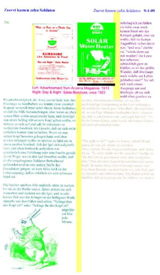
The most prevalent error found was sections of non-text being classified as both text and non-text. Figure 2.1 shows a page with two figures. The figure at the top of the page is a book colored bright green, red, orange, and blue. Similarly, the figure at the bottom is a rabbit colored bright green and blue. When the program was adjusted so that only non-text pixels were output, both figures were completely green, meaning all of the pixels were classified as non-text; however, when both types of pixels were output, multiple colors emerged in the figures, indicating that some pixels were considered both text and non-text.

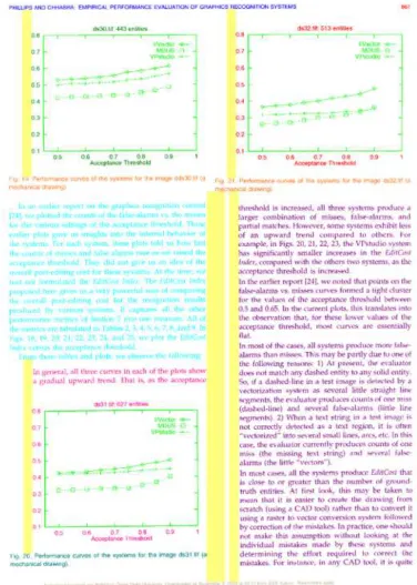
Graphs also tended to contain both text and non-text pixels; however, they did not overlap as in the case described in the previous paragraph. Figure 2.2 shows the output of a page taken from a scientific journal. The legends and axis labeling were classified as text, but the border, data, and data lines were classified as non-text.

(37)

(38)

19

(39)

be found for the OCR engine.

Based on this data, it was determined that the RAST algorithm could be improved by correcting the segmentation of non-text (e.g., half-tone images) so that text is not included, as well as properly identifying and segmenting graphs and tables. Since the goal of this thesis is to enable OCR of text areas, these regions need to be grouped properly and identified as non-text along with any encountered images. Once this is done, only text should be fed to the OCR engine. Also, since the images will be acquired using cameras with different resolutions, RAST needs to be robust enough to segment low resolution images as well. Therefore, the first goal of this thesis is to implement these improvements, ensuring that they perform at a range of resolutions as discussed in Section 3.3.

2.4 Voronoi Basis

The Voronoi module of OCRopus, conceived and implemented by Kise et al. [13], was also run on the test documents discussed in Section 2.1. It is less sophisticated than RAST in that it does not classify the regions, so consequently it cannot place the text in reading order, which means there is no text output. As a segmentation algorithm, though, it works fairly well. While it does not identify columns, it groups blocks of text in different columns correctly and usually creates separate segments for picture captions.

(40)

21

(41)

contains at least four additional regions.

The output of the scientific paper containing graphs is shown in Figure 2.5. Each of the graphs contains four to twelve regions within the boxed area, as well as individual regions for each of the axis numbers and labels when only one region should be created for each graph.

The last example, shown in Figure 2.6, illustrates the output of the document containing a table. The table is oversegmented along the columns as in the RAST case; however, the titles are not included in the column regions.

In terms of zone classification, a number of papers have been written on the subject. The paper documenting the Voronoi method itself [13] states that the zones were classified as either text or non-text in their study; however, it is not clear how this was done. From what the author can discern, it may have been when the lines between the characters were deleted, thus assigning the area containing those lines the class text.

Two other groups of researchers report classifying segmented regions using neural networks [26, 27]. First, they extract the connected components, then they segment the image into regions using either a RXYC or RLSA method. Then, based on the bounding boxes of the connected components, they use features including the amount of overlap between boxes, the amount of touching between boxes, the fill ratio of the boxes (number of black pixels to box area), the dimensions (height, aspect ratio, and size) of the boxes, the ratio of black to white pixels, the number of horizontal transitions from black to white pixels, the length of the horizontal run of black pixels, and the angle subtended from the lower-left corner to the upper-right corner to classify the regions using a neural network.

(42)

his-23

(43)

(44)

25

(45)

tograms (Tamara texture, relational invariant feature, run-length of black and white pixels in eight different directions, heights, widths and separations of the bounding boxes) and other aspects (fill ratio and the total number, mean and variance of black and white pixel runs) as the features. This method is also accurate, but as in the previous method, determining the values of all of the features is time consuming, and thus, since this the focus of this thesis is on page segmentation rather than region classification, a simpler approach was sought.

(46)

27

CHAPTER 3 DESIGN AND IMPLEMENTATION

This chapter covers the algorithm development and implementation details of the comparison program, XML output in OCRopus, RAST page segmentation, and Voronoi page segmentation. Based on the method described in Section 2.1, a compar-ison program was implemented and tested iteratively to ensure the correct analysis of various types of errors. Since it was to be used as the metric for both algorithms, it was imperative that it be correct. On the other hand, introducing XML output to the OCRopus program was straightforward and is explained in Section 3.2.

Once OCRopus could output XML page regions and they could be compared to the ground truth, the algorithms were developed. Since the RAST algorithm was more sophisticated than the Voronoi algorithm, it was addressed first. A collection of different types of documents were processed by it and their segmentations evaluated. The most frequently occurring errors were addressed first by introducing additional steps in the algorithm, running more tests, then analyzing the results. This process was repeated until satisfactory performance levels were achieved at 300 DPI.

(47)

As for the Voronoi algorithm, since it did not classify the regions, this functionality needed to be added first. After this was done, it was possible to address the quality of the segments themselves in terms of oversegmentation using a selection of different documents. Since non-text areas suffered from this problem the majority of the time, the algorithm only needed to treat the non-text regions. Once the regions were segmented properly, resolution issues were resolved as in the RAST algorithm.

3.1 Comparison Program Implementation

The first step in comparing detected regions to ground truth is parsing the XML files. There are two ways this can be done in C++: SAX (Simple API for XML) and DOM (Document Object Model) [25]. The SAX method involves event-based parsing where either callback functions or an object that implements various methods are created and, as certain tags are encountered, actions are taken. The DOM method, on the other hand, creates a tree data structure while parsing the file so that the elements and their descendants can be accessed repeatedly. Since this method essentially has built-in parsing functionality, it was chosen for this program.

As written earlier, each XML file contains a list of zones corresponding to the seg-mented regions of the page. Each of the zones has the following tags: “ZoneCorners,” “Vertex,” “Classification,” and “CategoryValue.” Figure 3.1 illustrates how a file with two zones would be structured. The information for the zones is kept in the leaves of the tree. So, in this case, the “Vertex” leaves contain the coordinates of the corners of the rectangles and the “CategoryValue” leaf contains the class of the zone (i.e., “Text” or “Non-text”).

(48)

29

Figure 3.1: XML file data structure.

examined and placed into a custom Rect object that has attributes for the vertices and classification. It is shown in detail in Appendix A. A two-dimensional array, or vector, ofRectsis then created to house the objects where one dimension corresponds to the class of the zone and the other to the number of the zone. In this way, the statistics for each class can be tabulated easily.

Following Rect vector construction, the work of comparing the data files begins. The first step is to calculate the match scores of each of the regions and place them into a two-dimensional array where one dimension represents the ground truth regions and the other the detected regions. Each of the regions is considered in turn and the amount of overlap between it and each of the other regions is calculated. The overlap is determined by comparing the vertices of each rectangle then summing the pixels in the area of overlap, if any. The match score is the amount of overlap divided by the area of the larger rectangle.

(49)

Figure 3.2: Example of Match Score tables - actual value on the left, thresholded on the right - and G and D-profiles. Taken from page 851 of [24].

regions along one direction (i.e., horizontal) and the detected regions along the other (i.e., vertical). If one were to sum the thresholded match scores for each region in each direction, Ground Truth and Detected profiles could be constructed for each of the regions. An illustration of the tables and the G/D-profiles is shown in Figure 3.2. Now that the groundwork has been laid, counts of the one-to-one, many-to-one, and one-to-many matches can be calculated. First, the easy one-to-one matches are counted by adding up the thresholded match scores equal to one that have corresponding G and D-profiles of one, meaning they are perfect matches. For each case meeting this criteria, the corresponding G and D-profiles are set to -1 so that they are not reconsidered.

(50)

31

match score is selected as the matching one. After this, regions matching the above criteria, with the exception that the D-profile must be greater than one, are considered and selected in the same fashion. In both cases, the G and D-profiles are set to -1 upon selection of the match and the profiles of the runners up are decremented by one.

Following the resolution of many-to-one detected regions, the one-to-many de-tected regions are resolved in a similar fashion. In this case, the best candidates with D-profiles equal or exceeding two and G-profiles greater than zero are selected. Then, the opposite cases are considered, where D-profiles are greater than zero and G-profiles are equal to or exceed two.

After all of the one-to-one matches are tallied, the program counts the detected one-to-many and many-to-one, as well as ground truth one-to-many and many-to-one matches. This is done by pooling all of the ground truth regions with match scores above the user-given rejection threshold for each of the detected regions. If the sum of the match scores exceeds the acceptance threshold for the detected region under consideration, it is deemed a one-to-many detected match. The number of corresponding ground truth regions is then added to the ground truth many-to-one match count. The same algorithm applies to calculating ground truth one-to-many and detected many-to-one matches.

(51)

3.2 Implementation of XML Output

Since the classification of OCRopus’ segments is rendered by coloring the pixels and outputting them to a PNG image file, but the comparison program requires XML files, a module was added to OCRopus to create and output the regions in XML format.

Starting with the default RAST module of OCRopus, the columns of text and graphics boxes correspond to the ”Text” and ”Non-text” regions of the page. There-fore, the easiest way to output the segmentation data to an XML file is to export these rectangles. After the column separators, or gutters, are found, the horizontal and vertical rulings, along with the graphics, are extracted from the connected components of the image. At this point, the text lines are found using this data and parameters gleaned from the statistics of the connected components (i.e., the estimated height and width of a text line). Then, the text lines are sorted into reading order and the columns are found.

After fixing a couple bugs in the original implementation and making some minors edits to the ”get-text-columns” function in ocropus/ocr-layout/

ocr-detect-columns.cc, the text blocks could be defined properly (i.e., where all are included, but non-text areas are excluded). Then, the non-text regions are passed to thehps_dump_regionsfunction of the newocropus/ocr-layout/ocr-hps-output.cc

(52)

33

3.3 Mixed-Content RAST Algorithm

Once OCRopus was capable of producing output in the correct format, the page segmentation algorithm itself was addressed. While RAST was designed for text-only documents, it does partially support text/non-text segmentation. It divides pixels into groups of text, non-text, gutters, and rulings; however, some of the pixels can be classified as both text and non-text. It starts by binarizing the page, extracting the connected components, then determining the bounding boxes of each of them. At this point, it calculates some statistics for the boxes, including height and width, and uses them to determine whether or not each of the boxes contains a character. Those that do contain characters are called character boxes and are saved into an array.

Next, the original algorithm computes the whitespace covers (i.e., white rectangles, a.k.a., gutters) of the page using statistics dervived from the character boxes. Then, the non-text pixels, which are classified as either graphics or horizontal/vertical rulings, are extracted from the large components. All of these items, with the exception of the horizontal rulings, are placed into an array representing text-line obstacles.

(53)

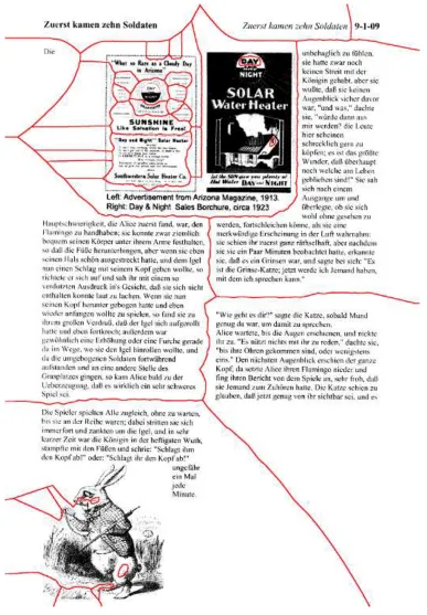
Then, the author added new functionality to the RAST algorithm. Since one of the observed deficiencies of the algorithm was the dual labeling of pixels as shown in Figure 2.1, the first improvement was made to the text-line extraction function. Where it filters out character boxes that lie within gutters, it now also filters out character boxes that are additionally labeled non-text. So, the ”character boxes” that actually contain connected components that are not characters can no longer be used to build text lines.

It was also discovered that character boxes not overlapped by the bounding boxes of any text lines, as shown in Figure 3.3, were dropped from consideration completely. So, the new algorithm now captures, closes (i.e., dilates, merges, then erodes [29]), then adds them to the non-text array of boxes. The amount of dilation is one fourth of the height of an average text-line box so that only ”character boxes” in close proximity to each other are merged. Another problem was that gray areas of images were not being classified as non-text. So, isolated pixels and very small bounding boxes, such as those shown in Figure 3.4, are now saved, closed (using the same amount of dilation as the non-character boxes), and added to the non-text array as well.

(54)

35

(55)

(56)

37

The new process outlined above starts by merging text boxes that overlap other text boxes then relabeling their union as non-text. Then, small non-text boxes (i.e., below a threshold of 10% of the square of the height of an average text line) are filtered out, since they most likely correspond to noise in the document image.

At this point, the improved algorithm iterates through a series of three steps until the array of non-text boxes is stable. First, text lines that overlap non-text boxes are reclassified as non-text. Second, non-text boxes that overlap other non-text boxes are merged, and third, non-text boxes are closed so that isolated boxes are merged. Since the second and third steps can cause non-text boxes to overlap text boxes, the first step is run again. Similarly, since the first step can cause newly created non-text boxes, to overlap other non-text boxes the second and third steps need to be repeated. Therefore, the algorithm iterates through all three steps until no more boxes are reclassified or merged.

Figure 3.5 illustrates the picture of the book previously shown in Figure 2.1. The boxes outlined in blue indicate the non-text boxes prior to manipulation. Note the large number of boxes including a nested set in the upper-left corner. There are also many overlapping boxes on the right side of the figure, although they are difficult to see against the black area of the figure. Figure 3.6 shows the same figure after the text and non-text boxes have been manipulated as discussed earlier. Now there is only one non-text box, which covers the entire figure.

(57)

Figure 3.5: Non-text boxes before converting text boxes, merging and closing.

(58)

39

was reset to a multiple of the width of this box.

Further testing using this new definition, however, revealed that the box width itself was not reliable. It was calculated by examining the histogram of the widths of the boxes and assigning the value of the first peak. Visual examination of the histograms of several images, though, indicated that the value of the first peak was much smaller than the width of a typical character. This even occurred in images not containing pictures, since the bounding boxes of periods, commas, apostrophes, and noise elements make up a significant portion of the histogram. Therefore, it is necessary to take the value of the next peak instead, which in the case of width corresponds to the right-most peak. In the case of height, it also corresponds to the right-most peak, but it is the third, not the second peak, because the second corresponds to the height of x-height characters (i.e., a, e, o, u, etc.), unless all of the text is capitalized.

Finding the correct peaks is not a simple matter. The histogram contains many local maxima that the program can mistakenly interpret as the peak of choice. Therefore, it needs to be smoothed until spurious local maxima disappear; however, it cannot be smoothed too much or the peaks themselves merge into one. So, the next step is to iteratively smooth the histogram until the expected number of peaks results. Then, the value of the right-most peak is obtained and assigned the box’s height or width depending on the type of histogram. Figure 3.7 illustrates iterative smoothing until only three peaks remain.

(59)

(60)

41

1. Binarize image.

2. Extract Connected Components (CC). 3. Calculate bounding boxes of CC’s.

4. Get character boxes and calculate statistics using iterative smoothing. 5. Compute whitespace covers.

6. Find gutters.

7. Classify large CC’s as either rulings or graphics. 8. Extract text lines ignoring graphics pixels.

9. Capture, merge and reclassify rejected character boxes as graphics. 10. Capture, merge and reclassify very small CC’s as graphics.

11. Merge overlapping text lines then reclassify as graphics. 12. Filter out very small graphics.

13. Merge text and graphics.

(a) Merge and reclassify text lines that overlap graphics. (b) Merge overlapping graphics.

(c) Close graphics rectangles. 14. Sort text lines into reading order.

15. Add gutters that do not overlap graphics and vertical rulings to vertical separa-tors.

16. Group text lines into text regions (columns).

17. Group text and graphics regions in XML format.

(61)

3.4 Voronoi Page Segmentation with Classification

As written earlier, Voronoi page segmentation was not fully implemented in OCRopus. That is, users could segment document images into Voronoi zones, but they were not classified as text or non-text so could not be appropriately routed to the OCR engine. Frequent oversegmentation of zones has also been demonstrated. Additionally, since XML output is required to measure the accuracy of the page segmentation, the segmentation needed to be converted to this format as well.

Addressing all three concerns, the algorithm was extended in three steps: clas-sification of the zones, merging of non-text zones, and clean up of any overlapping non-text regions (note that the term ”zones” corresponds to geometries created by the basic Voronoi algorithm and ”regions” corresponds to page segments). The original algorithm starts by binarizing the image, finding the Voronoi zones, numbering them, and creating an image of the numbered zones as depicted in Figure 3.9. At this point, the original Voronoi algorithm ends and the new algorithm developed by the author begins. The first step of the new algorithm is to save the interior zone boundary lines into another image as shown in Figure 3.10.

(62)

43

(63)

(64)

45

Figure 3.11: The ”text rectangle” of an unclassified zone.

contain text, and based on this information, classify the zone as text or non-text. The classification algorithm begins by creating a histogram of the locations of the lower-left corners (y0-values) of the character boxes so that it can determine the average location (or y-value) of each text line. A section of the histogram obtained from zone #8 of Figure 3.9 is shown in Figure 3.12. Notice that there exist shorter peaks to the left of each major peak. These correspond to the y0-values of descenders (i.e., letters that extend below the line like g, j, y). Since these values do not represent the location of the line, they need to be discarded, but in order to do this, the threshold under which they exist needs to be determined. This is done in a four-step process developed by the author.

(65)

Figure 3.12: Section of the histogram of the y0-values of the character boxes of zone #8 in Figure 3.9. The peaks to the left correspond to letters extending below the line and the peaks to the right correspond to letters sitting on the line.

Figure 3.13: Section of the smoothed histogram of Figure 3.12.

peak is selected, which is twelve in this case. Half of this value is then used as the threshold for finding the peaks of the original histogram.

Once the y-values of the text lines have been found, the character boxes lying within a certain distance of each line (i.e., the width of an average character box) are found. For each line, the widths of the associated character boxes are summed and the x-values over which they extend is calculated. Densities for each line are then determined as the sum of the widths of the character boxes divided by their x-extent. If 80% of the lines have densities exceeding 50%, the zone is classified as text.

(66)

47

Figure 3.14: Histogram of the peaks of the y0-values of the histogram of Figure 3.13. In this example, for each of the lines, the median number of occurrences of the main y0-value is twelve.

each zone are placed into an array and their perimeters and found by dilating the Voronoi lines and ANDing them with the zone pixels. These pixels are then placed into another array. At this point, one of the non-text zones is selected and its non-text neighbors are merged with it recursively.

Part (a) of Figure 3.15 shows an oversegmented non-text region where the selected zone is colored red. To find its neighbors, the extreme upper, lower, left-most, and right-most perimeter pixels are identified and the pixels in the directions of the border are explored. For example, when the top pixel is under consideration, the pixels directly above it are explored. Since the width of the Voronoi lines are five pixels, the first five or so will correspond to the line; however, at some point after this, the exploration will encounter a pixel in a different zone. Based on this information, the identity of the neighbor is found, after which its label is updated to match the first zone’s.

(67)

(a) (b) (c) (d)

Figure 3.15: Zone coloring of non-text relabeling process. a) Initial zone coloring, b) after the smallest has been relabeled, c) after its neighbor has been relabeled and d) after all of the neighboring non-text zones have been relabeled.

At this point, the next non-text zone that has not been evaluated is considered and its neighbors converted to its zone number, and so on.

Following the merging of non-text zones, the algorithm enters the clean-up phase. This is most easily done in rectangle space rather than pixel space since it involves merging overlapping rectangles. So, the upper, lower, left-most, and right-most pixels of each zone are found and used to define the inner rectangles.

The first step of the clean-up addresses all of the text rectangles that are com-pletely covered by non-text rectangles. This is done by iterating through the rect-angles and checking for complete overlaps. Completely covered text rectrect-angles are simply deleted. The next step is to check for the opposite: resolve all non-text rect-angles that are completely covered by text rectrect-angles. In this case, the encompassing text rectangles are relabeled as non-text and the covered non-text rectangles are deleted.

(68)

49

the text overlaps (i.e., in the upper-right and lower-left quadrants of the original non-text rectangle). Figures 3.18 and 3.19 show the second case where the oversized text rectangle is broken up into smaller rectangles to avoid overlapping the figure.

Once the algorithm was completed, it was tested at resolutions other than 300 DPI. At 200 DPI, the performance was slightly lower, but not appreciably and could be attributed to the loss of detail in the file; however, at 600 DPI, the performance dropped dramatically and was traced to the hard-coded parameter used to define noise pixels in the document. That parameter was changed to a fraction (1/326,774, which was determined based on the hard-coded value for 300 DPI) of the number of pixels on the page after which the segmentation performance improved.

(69)

(70)

51

(71)

Figure 3.18: Wrap around text zone covers picture.

(72)

53

1. Binarize image.

2. Create Voronoi area diagram then number each zone. 3. Extract Connected Components (CC).

4. Calculate bounding boxes of CC’s.

5. Get character boxes and calculate statistics using iterative smoothing. 6. Place non-overlapping character boxes into an array.

7. Zones are labeled to be text or non-text and rectangular zones are created.

(a) Find the most frequently occurring y-values (text line locations). (b) Sort the boxes into text lines.

(c) Calculate the density of the boxes for each text line.

(d) If the density of 80% of the lines is at least 50% label as text. 8. Dilate the line pixels then AND them with the zone pixels to find the

perimeter pixels. Place these and the zone pixels into two separate arrays.

9. Iterate through the non-text zones merging neighboring zones. For each non-text zone, use its perimeter pixels to explore outward and find its neighbors. Then relabel them with the original zone’s label. The labeling method is recursive whereby after relabeling the given zone it finds its neighbors and relabels all of them and so on.

10. Clean up the segmentation.

(a) Text zones which are completely overlapped by non-text zones are deleted.

(b) Non-text zones which are completely overlapped by text zones are deleted and the text zones are reclassified as non-text.

(c) Non-text zones which have merged across column dividers are broken so that they do not overlap neighboring text.

(d) Text zones which partially overlap figures (wrap around text) are segmented.

(73)

CHAPTER 4 TESTING AND ANALYSIS

This chapter covers the testing and analysis of the implementations of the improved RAST and Voronoi algorithms. 450 text documents were created comprising eight different types (i.e., single column, double column, etc.) and a range of resolutions. Then, their associated ground truth XML files were generated. These documents were used to test and analyze the algorithms such that the comparison program gave an overall metric and TrueViz provided a means to visualize the results. Using these tools, the algorithms were analyzed in terms of types of errors, both across and specific to particular classes, as well as a function of resolution.

4.1 Test Documents

(74)

55

column text only (10x5), single column text with half-tone images (10x5), double column text with half-tone images (10x5), and a mixture of single and double columns with half-tone images (10x5). The rest of the data set includes 50 pages taken from magazines (10x5) and 100 pages of technical journals that contain graphs, figures, tables and a title/abstract combination (20x5).

While the RAST and Voronoi algorithms were being developed, they were tested on a subset of the collection. Ground truth XML files were generated for each of the documents from the TIFF files so they could be compared using the comparison tool. Testing started from the first class and progressed to the most complex at a resolution of 300 DPI, using the PNG file format. Once the algorithms demonstrated acceptable performance levels at 300 DPI, they were analyzed at the remaining resolutions. If the performance dropped off, the algorithm was examined for resolution-dependent parameters and modified to be resolution independent as discussed in Section 3.3. Following the testing of the improved RAST and Voronoi algorithms, ABBYY’s FineReader OCR package was evaluated to see how well a commercial program could analyze these types of layouts.

4.2 RAST Analysis

(75)

The graphs on the left illustrate the performance levels using the same weights as those used in the ICDAR 2007 Page Segmentation Competition [19] (1.0, 0.75, 0.75, 1.0, 0.75, and 0.75 for w1 through w6, respectively) for Equations 2.3 and 2.4; whereas, the graphs on the right depict the performance levels using the following weights: 1.0, 1.12, 1.0, 1.0, 1.0 and 1.12 for w1 through w6, respectively. For this algorithm, the results using the two different sets of weights are fairly similar.

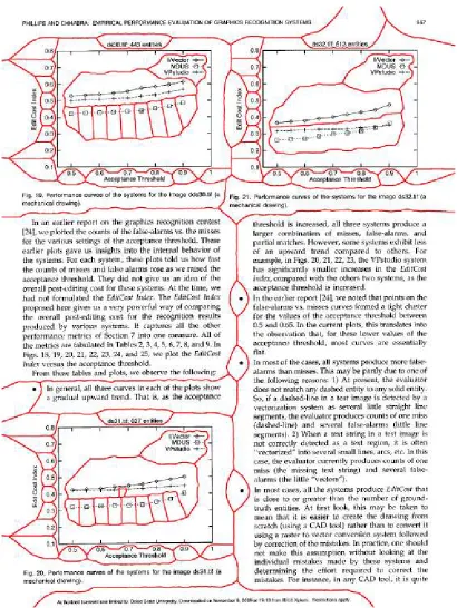
Examining these plots, the single, double, and mixed column text-only pages were segmented fairly accurately, from 80-100%, by the original RAST algorithm; however, the performance level of the documents containing half-tone images peaked between 30-60% at 100 DPI, then dropped at higher resolutions. There are two issues to address here: 1) is 100 DPI a feasible resolution with which to image a document, and 2) why does the performance drop after 100 DPI? Addressing the first issue, 100 DPI is a low resolution at which most detail in a document is lost, in which case it may not even be possible to recognize the characters.

In order to assess the lowest resolution at which the OCRopus OCR engine could produce reliable output, the author scanned a single column, text-only document at eight resolutions and ran them through the OCR engine. Table 4.1 shows that at 100 DPI, the OCR engine could not recognize any of the characters. Therefore, the segmentation algorithms were not expected to perform at or below 100 DPI.

Regarding the second issue, while improving the RAST algorithm, the author found that the parameter used to specify the minimum length of the text lines was hard coded. As mentioned in Section 3.2, it was replaced by a multiple of the average character box height gleaned from the box width histograms.

(76)

57

(77)

Resolution (DPI) OCR results 300 missed 1 line 266 missed 2 lines 240 missed 3 lines 200 missed 2 lines 150 missed 18 lines

96 no output

72 no output

50 no output

Table 4.1: The performance of the OCR engine of OCRopus on a single column, text-only document for a series of image resolutions.

higher resolutions as well. The single, double, and mixed column documents with half-tone images show the most improvement from 30-60% to 80-90%. The segmentation of the technical documents improved on the order of 25% from approximately 40% to 60-70%. They did not improve as much because they contain graphs and tables that are discontinuous and difficult to capture completely as non-text.

The axes labels of the graphs tend to be misclassified or completely dropped, and the text in the tables tends to be classified as text. Since they actually are text, one might argue that they should be classified as such anyway; however, mechanisms would be needed to be added to handle their reading order for the OCR engine. So, they were treated as non-text in this thesis. The magazine class improved the least amount from 50% to 65% due to text/non-text merging, which will be explained shortly.

(78)

59

of the left column that has been defined as one region. It is slightly longer than the line above and below it, so it was not assigned to the same text column in the ”get-text-columns” function.

The second type of error was the merging of text regions as depicted in Figure 4.3. In this case, as in all of the cases, they were short columns. The reason why short columns were merged is because the function to find white spaces, some of which are later turned into column separators, examines their aspect ratios and rejects those below a certain threshold. So, short columns are not separated by gutters. This could be fixed by reducing the expected aspect ratio.

The last type of error involved merging text and non-text regions. This occurred in three different cases: when text wrapped around the figure in a non-linear fashion, when the column was very narrow, and when non-text was incorrectly detected in text regions. In the first case, RAST was not designed to handle non-Manhattan geometries and XML output does not support it either, so this type of layout is beyond the scope of this thesis. Therefore, that type of error was not addressed. In the second case, RAST did not recognize the text as columns because they were too narrow to be defined as text lines. This is a limitation of the algorithm because the dimensions of text lines must pass certain threshold tests.

(79)

(80)

61