STRUCTURES
by
Stephanie Potter
A thesis
submitted in partial fulfillment of the requirements for the degree of
Master of Science in Mathematics Boise State University
When one thinks of objects with a significant level of symmetry it is natural to expect there to be a simple classification. However, this leads to an interesting problem in that research has revealed the existence of highly symmetric objects which are very complex when considered within the framework of Borel complexity. The tension between these two seemingly contradictory notions leads to a wealth of natural questions which have yet to be answered.
Borel complexity theory is an area of logic where the relative complexities of classification problems are studied. Within this theory, we regard a classification problem as an equivalence relation on a Polish space. An example of such is the isomorphism relation on the class of countable groups. The notion of a Borel reduction allows one to compare complexities of various classification problems.
The central aim of this research is to determine the Borel complexities of various classes of vertex-transitive structures, or structures for which every pair or elements are equivalent under some element of its automorphism group. John Clemens has shown that the class of vertex-transitive graphs has maximum possible complexity, namely Borel completeness. On the other hand, we show that the class of vertex-transitive linear orderings does not.
We explore this phenomenon further by considering other natural classes of vertex-transitive structures such as tournaments and partial orderings. In doing so, we discover that several other complexities arise for classes of vertex-transitive structures.
ABSTRACT . . . iv
LIST OF FIGURES . . . vi
1 Introduction . . . 1
2 Vertex-Transitive Graphs and Partial Orders . . . 8
3 Vertex-Transitive Linear Orderings . . . 19
4 Vertex-Transitive Tournaments . . . 29
REFERENCES . . . 36
1.1 Hierarchy of relevant benchmark equivalence relations . . . 3
1.2 Structures studied in this thesis . . . 5
2.1 Depiction ofuiRuj with ui =gpN and uj =gqN . . . 11
2.2 Graph ofM as constructed by Mekler, [8] . . . 13
2.3 Resulting square if there exist k1, k2 ∈N with vk1 adjvk2 ∈G. . . 15
4.1 Directed edges from vertex (0,0) to vertices one column to the right. . . 32
CHAPTER 1
INTRODUCTION
Classification problems in Mathematics ask the question: “How can objects of a given type be identified and distinguished from one another, up to some equivalence relation?”
When one thinks of objects with a significant level of symmetry it is natural to expect there to be a simple classification. However, this leads to an interesting problem in that research has revealed the existence of highly symmetric objects which are very complex when considered within the framework of Borel complexity. The tension between these two seemingly contradictory notions leads to a wealth of natural questions which have yet to be answered. In this thesis we will answer some of these questions in an attempt to further understand where vertex-transitive structures lie in terms of Borel complexity theory.
Borel complexity theory is an area of logic where the relative complexities of classification problems are studied. Within this theory, we regard a classification problem as an equivalence relation on a Polish space. An example of such is the isomorphism relation on the class of countable groups.
Definition 1. Let L = {Ri : i ≤ I} be a finite relational language, where Ri has arity ni. Denote the space of all countable L-models as Mod(L). Each element of Mod(L) can be viewed as an element of the product space
XL=
Y
i≤I 2Nni.
That is, for every x ∈XL let Mx ∈ Mod(L) be the countable model coded by x. Then for any i ∈ I and (k1, . . . , kni) ∈ Nni, it is the case that RMxi (k1, . . . , kni) ⇔
xi(k1, . . . , kni) = 1. For the remainder of this paper we will identify Mod(L) andXL.
Definition 2. The logic action of S∞ on Mod(L) is defined by letting g·M =N if
and only if
RNi (k1, . . . , kni)⇔RMi (g
−1(k
1), . . . , g−1(kni))
for all i ∈ I and (k1, . . . , kni) ∈ Nni. Therefore, g ·M = N if and only if g is an isomorphism from M onto N.
Definition 3. An invariant Borel class of countable L-structures is an S∞
-invariant Borel subset of Mod(L).
Note that for the purposes of this thesis we always study the orbit equivalence relation, i.e. the isomorphism relation on either Mod(L) or on the invariant Borel class.
Definition 4. Let E and F be equivalence relations on the Borel spaces X and Y
respectively. E is considered Borel reducible to F, denoted E ≤B F, if there exists a Borel function f :X →Y such that, for x, y ∈X, xEy if and only if f(x)F f(y).
E and F are bireducible to each other, denoted E ∼B F, if both E ≤B F and
F ≤B E.
Borel reducibility allows for organization of complexities into a hierarchy. The figure below shows the Borel reductions between the benchmark equivalence relations which are relevant to this thesis.
Borel Complete
E0 Eω1
id(2ω) id(ω)
Figure 1.1: Hierarchy of relevant benchmark equivalence relations
These equivalence relations are increasing in the sense of Borel reducibility from bottom to top wherever there is an edge. We also note that there are many equivalence relations that lie in between those shown which are omitted for the purpose of readability.
We then see that there exists a Borel reduction from id(ω) to id(2ω), or equality on an uncountable Polish space. Note that, for an equivalence relation E on a setX,
E is said to be smooth if it is the case thatE is Borel reducible to id(2ω).
In addition, we see that id(ω) is less complex than Eω1, or isomorphism on codes
for countable ordinals.
Increasing in complexity, we arrive at the equivalence relation E0 which is the
immediate successor to id(2ω), among the Borel equivalence relations.
Definition 5. The equivalence relation E0 is the relation of eventual equality on 2ω.
That is,
xE0y⇔ ∃m∀n ≥mx(n) = y(n).
At the “top” of our Borel hierarchy, we have Borel complete which is the maximum possible complexity among isomorphism problems for countable structures.
Definition 6. Given C an invariant Borel class, C is Borel complete if and only
if, for every invariant Borel class B, B is Borel reducible to C.
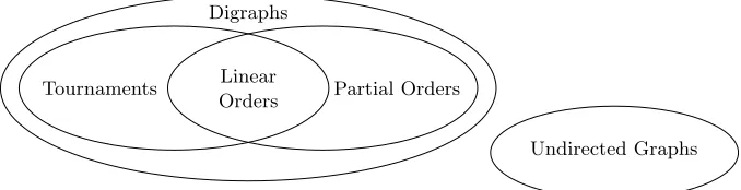
Some commonly referenced examples of Borel complete classes include the class of linear orders [3] and the class of directed graphs [4].
Digraphs
Tournaments Linear Partial Orders
Orders
Undirected Graphs
Figure 1.2: Structures studied in this thesis
It is important to remark that the class of vertex-transitive structures need not be Borel. To say that the isomorphism relation for such structures is Borel complete, it is sufficient to show that some Borel complete equivalence relation is Borel reducible to it. Formally, we give the following definitions of the structures seen in the figure above.
Definition 7. A graph is a pair of sets (V, E) where V is a set of vertices and E
is a set of edges formed by pairs of vertices in V. A directed graph, or digraph,
is a graph in which edges are ordered pairs, where edge (u, v) means that there is a directed edge from vertex u to vertex v.
We note that, for our purposes, directed graphs have no self-loops and no bidi-rectional edges. Further, we see that all other structures can be realized as directed graphs. Narrowing our focus slightly, we find partial orders and tournaments.
Definition 8. A partial order is a binary relation ≤ on a set X which is:
i. reflexive: x≤x for all x∈X
ii. anti-symmetric: x≤y and y ≤x implies that x=y
Definition 9. A tournament is a directed graph in which every pair of distinct
vertices is connected by a single directed edge.
Finally, tournaments which satisfy the properties of partial orders are linear orders, and vice versa.
Definition 10. A linear order is a partial order ≤ on a set X which also satisfies
the comparability axiom. That is, for every x, y ∈X either x≤y or y≤x.
We begin by extending the results regarding vertex-transitive graphs in Clemens’ paper titled Isomorphism of homogeneous structures [1]. In this paper, Clemens showed that the isomorphism relation on countable, connected, vertex-transitive, undirected graphs is Borel complete. Morover, he suggested that one could also prove this for the directed case. Here, we first cover the simpler directed case before filling in the missing components needed to prove the original result for undirected graphs. A consequence of this leads to the result that vertex-transitive partial orders are Borel complete.
This analysis then leads us to ask about the complexity of a special case of directed graphs: linear orders. We have shown that the class of vertex-transitive linear orderings is, in fact, not Borel complete. Further, we see that there exists an absolutely ∆1
2 reduction from isomorphism on codes for countable ordinals, denoted
Eω1, to isomorphism on vertex-transitive linear orders.
We finish this paper by broadening our view slightly to consider vertex-transitive tournaments. That is, linear orders are a special type of tournament and so it is natural to see where tournaments lie in terms of Borel complexity. Here we show that isomorphism of vertex-transitive tournaments is properly more complex thanE0
Beyond the results given in this thesis it is natural to ask about other vertex-transitive structures. For example, linear orders are a particular type of lattice, which are partial orders. Since we know that isomorphism of linear orders is Borel complete and isomorphism of partial orders is, in fact, Borel complete it is natural to ask if the class of vertex-transitive lattices is Borel complete as well.
CHAPTER 2
VERTEX-TRANSITIVE GRAPHS AND PARTIAL
ORDERS
We begin by considering isomorphism of vertex-transitive graphs. The work shown here is an extension of results from Clemens’s paper titled Isomorphism of homogeneous structures [1] in which he first showed that the isomorphism problem for countable, connected, vertex-transitive graphs is Borel complete.
The aim is to break up the proof that the isomorphism problems of countable connected vertex-transitive graphs is Borel complete into several components in order to uncover further results which follow from Clemens’s ideas. We will first show that the class of extensional graphs is Borel complete. We then see that there exists a Borel reduction from the isomorphism relation on countable graphs to the isomorphism relation on countable, connected vertex-transitive graphs.
Definition 11. A connected graph is a graph in which there exists a path between
every pair of vertices. A directed graph isweakly-connectedif replacing all directed
edges with undirected edges results in a connected graph.
Theorem 12 (Extracted from [1]). There exists a Borel reduction from countable graphs to countable, weakly-connected, vertex-transitive, directed graphs.
Proof. Let hviii∈N enumerate the vertices of a countable graph G. Define H to be
the group generated freely by the the vertices of Gwith the stipulation that adjacent vertices commute. That is, let Fω be the free group on generators gi and N be the normal subgroup of Fω generated by {gigjg−i 1g
−1
j : vi adjvj in G}. Then, define
H =Fω/N and form Γ, the directed Cayley graph of H with generators hgiii∈N. The
vertices of Γ are left cosets of N in Fω and two vertices w1N and w2N are adjacent
in Γ if giw1N =w2N with a directed edge from w1N to w2N. Note that each of the generators gi are in distinct cosets.
In order to produce a code for this structure, we begin by fixing an enumeration hwiii∈N of words in Fω. For each coset of N we pick a representative for that coset
by picking the least i such that wi is in the given coset. This wi is the coset representative. Then, enumerate the chosen representatives and define the binary relation on N encoding Γ according to whether corresponding cosets are adjacent in Γ.
ϕ(wN) =wN w−11w2 =ww1−1w2N,
an automorphism of Γ sending w1N to w2N.
Now, suppose we have two isomorphic graphs G1 and G2 with f an isomorphism between them. LetN1 and N2 be the normal subgroups in the construction of Γ1 and
Γ2 respectively and let
ϕ(wN1) =wNe 2
where, for w= ginσn. . . gσ0
i0, we =g
σn f(in). . . g
σ0
f(i0). Well, f induces a partial map ϕfrom
their respective Cayley graphs ,Γ1 to Γ2, such thatϕ(giN1) = gf(i)N2 which acts on the
cosets of thegi. We then extend this partial map to an isomorphism on the graphs as a whole. Certainly, ϕis a bijection. To see that it is well-defined, note that the map taking w to we is an automorphism of Fw which sends N1 to N2 and so w1w2−1 ∈ N1
if and only if wf1fw2
−1
∈N2.
Now, suppose that w1N1 →w2N1 in Γ1 or, in other words,gkw1N1 =w2N1. Then ϕ gives that (^gkw1)N2 = w2N2f . Notice that g]kw1 = gf(k)w1f and so gf(k)ϕ(w1N1) =
ϕ(w2N1). The argument in the other direction is the same and so w1N1 →w2N1 in
Γ1 if and only if ϕ(w1N1)→ϕ(w2N1) in Γ2.
Finally, suppose that Γ1 and Γ2 are isomorphic. We want to show that G1 ∼=G2
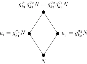
which can be achieved by seeing that one can recoverG(up to isomorphism) from the isomorphism class of Γ. Recalling that Γ is vertex-transitive, without loss of generality we can fix a vertex in Γ corresponding to N and identify its adjacent vertices, gkN. Enumerate these adjacent vertices ashuiii∈N. LetR be the binary relation on this set
uiRuj ⇔ ∃b6=N such thatui =giN →b and uj =gjN →b.
The aim is to show that uiRuj if and only if there exist p, q ∈ N with ui =gpN and
uj = gqN such that vp adjvq in G. Well, if such a pair p, q exists, then gp and gq commute in H. Then ui and uj are opposite corners of the square including N and
gqgpN =gpgqN. Thus uiRuj. Suppose now that uiRuj, with ui 6=uj. Let ui = gpN and uj = gqN with N and b = gngqN = gmgpN as the other two vertices of the square.
gpN gqN
b
N
Figure 2.1: Depiction of uiRuj with ui =gpN and uj =gqN
Thus it must be that
gp−1gm−1gngq ∈N. (2.1)
Recalling that words in N must have the sum of the exponents of each generator equal to 0, it must be that p= q and m =n or p =n and m =q. As ui 6=uj then
gpN 6= gqN and so it cannot be the case that p=q and m =n. Therefore, gp =gn and gm =gq and so
which means that vp adjvq ∈ G. Thus we can recover from Γ an isomorphic copy of
Gby taking the out-neighbors of N as the vertices andR as the edge relation and so the desired Borel reduction exists.
With this, we have that the isomorphism relation on countable, connected, di-rected vertex-transitive graphs is Borel complete. The proof of the undidi-rected case is very similar and so we exclude the redundancies. We also point out the additional cases required by not knowing whether the powers of thegi in equation (2.1) are 1 or −1. Additionally, this proof requires that the graphG be extensional.
Definition 13. An extensional graph is one in which, for any vertices v1 6= v2,
there exists a third vertex v3 such that v1 adjv3 and not v2 adjv3.
Fortunately, the following Lemma due to Mekler [8] tells us that the isomorphism relation on extensional graphs is also Borel complete. To prove this, note that the isomorphism relation of countableL0-structures is Borel complete [3], whereL0 is the
language containing a single binary relation symbol. We then show that there exists a Borel reduction from the isomorphism relation onL0-structures to extensional graphs
which gives the desired conclusion.
Lemma 14 (Mekler). There exists a Borel reduction from the isomorphism relation on L0-structures to the isomorphism relation on extensional graphs. Thus, the class
of extensional graphs is Borel complete.
Proof. LetAbe anL0-structure. First, buildG0(A) such that its vertices are elements
ofAand there are two nodes adjacent to each. IfAsatisfiesa1Ra2, introduce two new
vertices (a1,2)1 and (a1,2)2 such that a1 adj(a1,2)1, (a1,2)1 adj(a1,2)2, and (a1,2)2 adja2.
to (a1,2)2. The graph ofM constructed up to this point can be seen in the figure below.
Figure 2.2: Graph of M as constructed by Mekler, [8]
Finally, insert three new vertices adjacent to one another and to each of the previous vertices ofG0(A). Once G0(A) is constructed, let each element ofG0(A) be a vertex of G(A). G(A) is constructed by inserting a new vertex in the middle of each edge. Let hviii∈N enumerate the vertices of G(A). We note that G(A) is extensional.
In order to show that this Borel map is, in fact, a Borel reduction we must show that A1 ∼= A2 if and only if G(A1) ∼= G(A2). If A1 ∼= A2, then there exists an
isomorphismϕ:A1 →A2such that ifa1Ra2inA1thenϕ(a1)Rϕ(a2) inA2. Asa1Ra2,
we obtain the resulting encoding G(A1). Applying ϕto the vertices representing a1
and a2, we achieve an isomorphism ϕ0 sending vertices in G(A1) to vertices inG(A2)
and so G(A1)∼=G(A2).
Suppose now that G(A1)∼=G(A2). That is, there exists an isomorphism
ϕ0 : G(A1) → G(A2) sending structures representing adjacent vertices in A1 to
structures representing adjacent vertices in A2. Consider any pairs of elements a1 adja2 inA1 anda3 adja4 inA2. Then there exists an encoding in G(A1) ofa1 adja2
To see that we can recover the two vertices representing elements in A1, one can
locate all vertices which are a distance of two from vertices of degree four in G(A). From these, one can identify v1 andv2 representinga1 and a2 respectively as follows:
v1 and v2 have five vertices in between them, where v1 is a distance of two from a
vertex of degree eight and v2 is a distance of two from a vertex of degree nine. Thus,
by our encoding, we can recover that a1 adja2.
As these graphs are isomorphic, we get that there exists an isomorphism ϕ such that v1Rv2 with respect to the encoding if and only if ϕ(v1)Rϕ(v2) or, equivalently, v3Rv4. Thus, we arrive ata1 adja2if, and only if a3 adja4 and soA1 ∼=A2as expected.
Theorem 15 (Clemens). There exists a Borel reduction from extensional graphs G
to countable, connected, undirected, vertex-transitive graphs.
Proof. The proof of this result very closely parallels the proof of Theorem 12, except we form Γ, the undirected Cayley graph of H, where two vertices w1N and w2N are
adjacent in Γ if there exists a generatorgi such thatgiw1N =w2N orgiw2N =w1N.
We then continue to show that the map G 7→ Γ is the desired reduction. Showing that G1 ∼=G2 implies Γ1 ∼= Γ2 is the same as in the proof of Theorem 12.
In order to see that Γ1 ∼= Γ2 gives G1 ∼= G2 requires showing that G can be
recovered from Γ. This becomes slightly more involved than in the directed case. The argument begins the same; however, instead of the definition of the relation R
given above, for two distinct elements ui and uj in Γ we define R as
We then aim to show that uiRuj if and only if there exist k1, k2 ∈ N and σ1, σ2 ∈
{−1,1} with ui =gkσ11N and uj =g
σ2
k2N such that vk1 adjvk2 in G.
Well, if such a pair k1, k2 exists then gk1 and gk2 commute in H. Thus ui and uj
are at opposite corners of a square shared with N and gσ1
k1g
σ2
k2N = g
σ2
k2g
σ1
k1N and so
uiRuj.
ui =gkσ11N uj =gkσ22N
gσ1
k1g
σ2
k2N =g
σ2
k2g
σ1
k1N
N
Figure 2.3: Resulting square if there exist k1, k2 ∈N with vk1 adjvk2 ∈G
Now, suppose that uiRuj with ui = gkσ11N and uj = g
σ2
k2N and a, b the other
two vertices of the square. Thus there must exist generators gn1, gn2, gm1, gm2 and
τ1, τ2, ρ1, ρ2 ∈ {−1,1}such that
a =gτ1
n1g
σ1
k1N =g
τ2
n2g
σ2
k2N and b =g
ρ1
m1g
σ1
k1N =g
ρ2
m2g
σ2
k2N.
So we have
g−σ1
k1 g
−τ1
n1 g
τ2
n2g
σ2
k2 ∈N and g
−σ1
k1 g
−ρ1
m1 g
ρ2
m2g
σ2
As words in N must have the sum of the exponents of each generator equal to 0, then it must be that k1 = k2, k1 = n1, or k1 = n2. If k1 = k2 then it must be
that −σ1 = σ2. Otherwise, ui = gkσ11N and uj = gkσ22N would be the same. Further, this would require that n1 = n2 = k1 = k2 and so σ2−σ1 +τ2 −τ1 = 0. Well, then
we would need −σ1 = τ1 and so a = gk−1σ1g
σ1
k1N = N. In the case that k1 6= k2 and
k1 = n1, we get that −σ1 = τ1 and so, once again, a =g−k1σ1g
σ1
k1N = N. Finally, for
the case where k1 6= k2 and k1 = n2 it also must be the case that k2 = n1, σ1 =τ2,
and σ2 =τ1. Well, theng−k1σ1g
−σ2
k2 g
σ1
k1g
σ2
k2 ∈N and sovk1 adjvk2 inG.
Repeating the same argument for b, we see that either b = N or vk1 adjvk2 in G.
Recalling that a 6=b it must be the case that vk1 adjvk2 in G. Thus we can identify
pairs of elements{ui, uj}, so that they areR-related to all of the same elements. That is, we have identified pairs{gkN, g−k1N}. By extensionality, this will not identify any other pairs as, given gi and gj, i 6= j, there exists a gk which commutes with gi but not with gj and vice versa.
Therefore, we form the graph with these pairs as its vertices where two vertices are set adjacent if each element in the first pair is R-related to each element in the second pair. The relation R then gives that this graph is isomorphic to G.
Therefore, the isomorphism relation on countable, connected, vertex-transitive graphs is Borel complete. A further consequence is that vertex-transitive partial orders are also Borel complete. This can be seen by taking the transitive closure of the directed graph from Theorem 12 which will result in a partial order, as we will do below. First, we recall the definition of a partial order:
Definition 16. A partial orderis a relation which is reflexive, antisymmetric, and
Definition 17. The transitive closure of a directed graph G, denoted C(G), is a graph which contains an edge {u, v}whenever there is a directed path fromu tov, for
u, v ∈G as well as a path of length 0 from u to u.
It is important to note that the transitive closure of a directed graph does not always yield a partial order. For this to be the case, it must be that the directed graph has no cycles. For the following statement, we remind the reader that, in this paper, directed graphs have no cycles of length one or two.
Proposition 18. If G a directed graph, then the transitive closure C(G), is a partial order if, and only if, G has no directed cycles.
Proof. For the forward direction, supposeC(G) satisfies the requirements of a partial order. Further, suppose towards a contradiction that G contains a cycle such that
x1 ≤ x2 ≤ · · · ≤ xn ≤ x1 for x1, x2, . . . , xn vertices of G(A). However, as C(G) is antisymmetric, x1 ≤xi and xi ≤x1 gives x1 =xi for 1≤i≤n. Therefore, it cannot be the case that G has a cycle.
Now, suppose there exist no cycles in G. To show thatC(G) satisfies the require-ments of a partial order, we first note that the transitive closure is, in fact, transitive. Further, we assumed the relation on Awas reflexive and so C(G) remains transitive, as this does not affect single vertices but the relationship between two vertices. And finally, as there are no cycles inG it must be that there are no cycles inC(G) and so we achieve antisymmetry. Thus the transitive closure ofGadmits a partial order.
Corollary 19. There exists a Borel reduction from the isomorphism relation on
extensional graphsGto the isomorphism relation on countable vertex-transitive partial
Proof. Recalling Proposition 18, note that the directed graph Γ of Theorem 12 has no directed cycles and so the transitive closure, C(Γ), is a partial order. To see that Γ has no directed cycles, note that Γ is the directed Cayley graph of H in which, for all words w =w1. . . wk having generators g1, . . . , gk, if w = 1 in H then the sum of all exponents of each of the correspondinggi must equal 0. Therefore, the sum is not positive and so there cannot be a directed cycle.
Therefore, given Γ one can produce its transitive closure, C(Γ), which is a partial order. The aim is to show that Γ1 ∼= Γ2 if and only if C(Γ1)∼=C(Γ2). If Γ1 ∼= Γ2 then
we certainly have that C(Γ1)∼=C(Γ2) as transitive closure is isomorphism invariant.
So, now suppose that C(Γ1) ∼= C(Γ2). Given C(Γ) we want to show that we can
recover the original b∈Γ such thatN →b in Γ from any pointp∈C(Γ).
The claim is that the out-neighbors of N are all of the b∈Γ such that N →b in
C(Γ) and there does not exist a directed path of length greater than one from N to
b in C(Γ). This is the case as, if there did exist such a path in C(Γ) then we would have
b=gjN and b=gi1. . . ginN
which would mean that gi1. . . ging
−1
CHAPTER 3
VERTEX-TRANSITIVE LINEAR ORDERINGS
After classifying directed graphs in the previous chapter it is natural to ask about the complexity of special cases of directed graphs such as linear orders. The main theorem of this chapter isolates the complexity of vertex-transitive linear orders, in particular. Before presenting this result, it is necessary to discuss the condensation of linear orders. Condensation will be used in the main theorem in order to classify vertex-transitive linear orders by countable ordinals (refer to [9] for more details).
First, let us recall that a linear order is a partial order ≤ on a set X which also satisfies comparability: for every x, y ∈X, eitherx≤y or y≤x.
Definition 20. Let L be a linear ordering and let L0 be a collection of non-empty
intervals of L which partitions L, ordered by
I1 I2 if, for all x1 ∈I1, x2 ∈I2, x1 < x2.
L0 is called a condensation of L.
and this automorphism extends toC[L]. For our purposes, we will make use of finite condensation maps, where discrete intervals are condensed.
Definition 21. The finite condensation map of L is denoted
cF(x) ={y|[x, y] or [y, x] is finite}
for x∈L. Let cF[L] denote the condensation of L determined by the intervals cF(x) for all x∈L.
Note that cF(x) can be finite or, otherwise, has order type ω, ω∗ or Z. We call cF(x) the equivalence class of x. This condensation map will be used implicitly throughout this chapter. Considering more than a single condensation leads to the following iterative definitions.
Definition 22. We define an iterated condensation map with c1 =c as
(i) cα+1(x) = {y|c(cα(x)) =c(cα(y))}
(ii) Assume thatλis a limit ordinal and that for eachβ < λwe have defined for each
linear ordering A the condensation map cβ. Then we define the condensation map cλ by
cλ(x) = [{cβ(x)|β < λ}
Proposition 23. Let L be a linear ordering of cardinality κ. Then there exists an
ordinal α < κ+ such that cβ(x) =cα(x) for all x∈L and for all β ≥α.
Proof. If cα+1(x) = cα(x) for every x ∈ L, then cβ(x) = cα(x) for every β ≥ α. Thus, for some set S ={α|cα+1(x)6=cα(x) for somex∈L}, S is an initial segment of ordinals.
Further, for each α ∈ S, there exists a pair {x, y} of elements of L such that
cα(x)6=cα(y) butcα+1(x) =cα+1(y). SoS is an initial segment of the ordinals which
is in a one-to-one correspondence with a subset of L×L. Thus S has cardinality at most κ.
Therefore, α has cardinality κ and so κ ≤α ≤ κ+ [9]. Thus we have an α < κ+
such that cβ(x) =cα(x) for every x∈L and for every β ≥α.
Recalling that our aim is to understand vertex-transitive linear orders, we will show that there are two such classes of vertex-transitive linear orders, namely powers of Z and Q copies of powers of Z. This leads us to the following definition:
Definition 24. Given an ordinal β, Z0(β) consists of all β-sequences of elements of
Z which have only finitely many non-zero entries. That is
Z0(β) = {s:β →Z| {α:s(α)6= 0} is finite},
ordered by s t if s(µ) < t(µ) where µ is the largest ordinal γ < β for which
For a more intuitive definition of powers of Z, one can recursively construct a definition of Z0(β), which we will call Zβ, as follows:
Definition 25. (i) Z0 = 1 (ii) Zβ+1 =
Zβ ·ω∗+Zβ+Zβ·ω =Zβ·Z (iii) Zλ = (P
{Zγ·ω |γ < λ})∗+ 1 +P
{Zγ·ω |γ < λ} for limit ordinals λ.
Note that we define the sum of arbitrarily many linear orderings as follows. Let hI, Ribe a linear ordering and, for each i∈I, let hAi, Siibe a linear ordering. Then
P
i∈IAi is defined to be the linear ordering hC, Tiwith C=
S
i∈IAi and, for any two
c1, c2 ∈C
c1 <T c2 if (c1 ∈Ai and c2 ∈Aj and i <R j) or
(c1 ∈Ai and c2 ∈Ai and c1 <Si c2 for some i∈I).
Further, we define the product of two linear orders,hI, Ri and hA, Si as
A·I =X i∈I
A
where addition is as defined above.
The following proposition tells us that the previous definitions of powers of Zare, in fact, equivalent.
Proposition 26. For any ordinal β, Z0(β)∼=Zβ.
Proof. This is proved by induction on β. First, consider the case Z0(0) ∼= Z0. By
definition Z0 = 1 and so now Z0(0) = {s: 0→Z|∃N∀n≥N s(n) = 0} ∼= {∅} ∼= 1.
Now, suppose we have that Z0(β) = Zβ and let us show that the successor case
holds, i.e. Z0(β+ 1)∼=Zβ+1 below:
Zβ+1 =Zβ·Z ∼
=Z0(β)·Z (by assumption) ∼
={(s: (β)→Z, t∈Z)|∃N∀n ≥N s(n) = 0} =Z0(β+ 1).
Finally, for a limit ordinalλ, we claim thatZ0(λ) = {s:λ→Z|{α:s(α)6= 0} is finite}
and Zλ = (P
{Zγ·ω |γ < λ})∗
+ 1 +P
{Zγ·ω|γ < λ} are isomorphic.
To see this, let ∈ Z0(λ) denote the sequence s(α) = 0 for all α. This
corresponds to the “100 in the definition ofZλ. Next, thes∈
Z0(λ) such thats(0) >0
and s(α) = 0 for all α >0 are a copy ofZ0·ω =ω.
In general, the elements s∈Z0(λ) withs(γ)>0 ands(α) = 0 for all α > γ are a
copy of Zγ·ω. Thus, we account for the sum P
{Zγ·ω |γ < λ} in the definition of Zλ.
There is an analogous correspondence between sequences in Z0(λ) and the sum
(P
{Zγ·ω|γ < λ})∗. Thus,
Z0(λ)∼=Zλ for λ a limit ordinal. Therefore we conclude that, for any ordinal β, Z0(β)∼=Zβ.
Proposition 27. A single condensation of Zβ+1, for β+ 1< ω, reduces to
Zβ.
Proof. By definition of finite condensation, we see that
cZβ+1={(a, b)|b ∈Z}|a∈Zβ ∼=Zβ
and so a single condensation of Zβ+1 reduces to
Zβ in the case that β+ 1 < ω. Moreover, given sequences inZλ for some limit ordinalλwe see that condensations of such sequences behave as described in the following proposition.
Proposition 28. ForZλ ={s:λ→Z| {α :s(α)6= 0} is finite}, given two sequences
s, t∈Zλ
(i) c(s) =t|s[1,λ)=t[1,λ)
(ii) cγ(s) =t|s[γ,λ)=t[γ,λ) for each ordinal γ.
Proof. Let Zλ = {s:λ →
Z| {α :s(α)6= 0} is finite} and consider two sequences
s, t∈Zλ.
(i) First, suppose s [1,λ)= t [1,λ) and, without loss of generality, let s t. Then
we must have s(0)< t(0). If there exists a thirdr ∈Zλ andr differs at a latter point γ then it does from both s and t so either r s t or s t r. If
s r t then it must be that s(0) < r(0) < t(0) and there are only finitely many r such that this is the case. Therefore [s, t] is finite and so c(s) =c(t). Now, if we suppose that s [1,λ)6=t [1,λ) then there exists a last ordinal γ such
n > s(0) and there are infinitely many rn which satisfy this. Therefore, [s, t] is infinite and so c(s)6=c(t).
Therefore, we conclude that c(s) =t |s[1,λ)=t[1,λ) .
(ii) This case follows using a similar argument to (i) and induction on γ.
As we alluded to earlier in the chapter, there are two classes of vertex-transitive linear orders. In order to prove this, we require the following definitions about single elements of L.
Definition 29. Given a linear ordering L,
(i) x∈L isleft dense ifx is not the least element inL and if there is no greatest
element y < x
(ii) x ∈ L is right dense if x is not the greatest element in L and if there is no
least element y > x
(iii) x∈L isleft discrete if there exists a greatest y∈L such that y < xor if xis
the greatest element of L
(iv) x∈ L is right discrete if there exists a least y∈L such that y > x or if x is
the least element of L.
Note that, given some elementx∈L,xwill be either left/right dense or left/right discrete. This leads us to the following lemma, where we will see thatZβ and
Lemma 30. If a linear ordering L is vertex-transitive, then
(i) if one point is left or right dense then every point is and, in fact, L∼=Q (ii) if one point is left or right discrete then every point is, and every equivalence
class is a copy of the integers or L= 1.
Proof. By vertex-transitivity, if one point is left or right dense then every point must also be left or right dense, respectively.
(i) First, let a < b. If b is left dense then, given a sequence {bi}i∈N approaching b from the left, there must eventually be some n ∈ N such that a < bn < b. Therefore,Lis dense. Similarly, letb < abe right dense. Then, given a sequence {bi}i∈Napproaching bfrom the right, there must eventually be some n∈Nsuch
that b < bn< a. Once again, Lis dense.
AsLis a dense linear ordering, thenLis isomorphic toQ,Q∪ {∞},{−∞} ∪Q, or {−∞} ∪Q∪ {∞}. However, as L is also vertex-transitive there can be no first/last element and so it must be the case that L∼=Q.
(ii) Similar to above, vertex-transitivity tells us that if one point is left or right discrete then every point must be left or right discrete. Thus L is discrete and so every equivalence class is either a single point, a finite number of points, ω,
ω∗, or Z. As before, the vertex-transitivity of L requires that there exists no first/last element of any class and so we must have that every equivalence class is a copy of the integers in the case that L has more than one element.
vertex-transitive linear orders, it is natural to ask what happens when we reach such a fixed-point.
Proposition 31. Given a vertex-transitive linear order L, if c(x) = {x} for every
x∈L then L is isomorphic to either Q or 1.
Proof. Let L be a vertex-transitive linear order and c(x) = {x} for every x ∈ L. There are two cases to consider:
(i) If one point is left/right dense then, by Lemma 30, L∼=Q.
(ii) If one point is left/right discrete then Lemma 30 tells us that there are two possibilities. The first is that L = 1. Otherwise, every equivalence class of
L is a copy of the integers. However, if this is the case then, for any x ∈ L,
c(x) ={y|[x, y] or [y, x] is finite} 6={x} as every x∈Z is a finite distance from at least one other y ∈ Z. Thus we reach a contradiction and so if one point is left/right discrete at c(x) ={x} for every x∈L then L= 1.
By Proposition 23 we are able to conclude that for countable, vertex-transitive linear orders it takes countably many steps to arrive at a condensation fixed point. Further, by Proposition 31 the possible condensation fixed points are either 1 or Q. In summary, we arrive at the following theorem.
Theorem 32. If L is a countable vertex-transitive linear order then L is isomorphic
to either Zβ or Zβ ·Q for some β < ω1.
To conclude this chapter, we find that there exists an absolutely ∆1
2 reduction
Theorem 33. There exists an absolutely ∆1
2 reduction from isomorphism on codes
for countable ordinals to isomorphism on vertex-transitive linear orders.
Proof. The aim is to show that there exists a ∆12 map from codes for ordinals α to codes for Zα. We can construct such a map by recursion on α. Given a code <
L on
ω for L we define, for n, m∈ L·Z where n =hn0, n1i and m =hm0, m1i, n <L·Z m
if and only if n0 <Z m0 orn0 =m0 and n1 <Lm1. For limit stages, given a code for
a limit ordinal λ, together with a λ-sequence of codes for Zα, α < λ, we can produce a code for Zλ = (P
{Zγ·ω|γ < λ})∗+ 1 +P
{Zγ·ω|γ < λ} in a similar manner. It is not difficult to check that each step of this recursive construction is Borel. Further, it is well known that this implies we can construct a code for Zβ in an absolutely ∆1
2 fashion. For example, an infinite time turing machine (ITTM) can
easily be programmed to carry out the recursive construction, and ITTM-computable mappings are always absolutely∆1
2 (for the definition of ITTM and the statement of
CHAPTER 4
VERTEX-TRANSITIVE TOURNAMENTS
We now shift focus to the classification problem for vertex-transitive tournaments. As tournaments are a broader class than linear orders, but still a subset of the class of directed graphs it makes sense to consider the complexity of these structures as well. While the exact complexity of vertex-transitive tournaments is yet to be determined, the main result in this chapter states that isomorphism of vertex-transitive tourna-ments is properly more complex than E0, or eventual equality on 2ω. A remaining
question is to determine whether this is, in fact, Borel complete.
Definition 34. Atournament is a directed graph in which every pair of vertices is
connected by an edge.
Recall that a tournament is vertex-transitive if its automorphism groups acts transitively on the set of vertices. We denote the isomorphism relation over vertex-transitive tournaments as ∼=V T T.
Further, we note the following two relations which will be necessary in the proof of the main theorem. First, eventual equality on 2ω is denoted E0. More formally, we say
We will find that, instead of working with E0 directly, we will need to work with
a subset of the domain of EZ, or the shift equivalence on 2Z. That is,
xEZy ⇔ ∃m∀nx(n+m) =y(n)
In order to show that isomorphism of vertex-transitive tournaments is more com-plex than E0 we will see that the necessary reduction only works on a subset of the
domain of EZ. However, this makes it necessary to check that the restriction of EZ
to this subset remains as complex as E0 which leads us to the following proposition.
Proposition 35. E0 on 2ω is Borel bireducible to EZ C on 2Z for any comeager set
C.
Proof. First, we claim that EZ has a dense orbit. To see this, note that 2Z has the
topology with basic open setsVt =
x∈2Z |t⊂x . Recall that 2<ω is countable and
let {si}i∈ω enumerate 2
<ω. Further, we define x = _ s
1 _ s2 _ · · · _ si _ . . . where denotes the sequence of all 0 on ω∗. This x is certainly in 2Z and contains
an instance of every finite binary sequence. That is, given s∈2<ω, there exists some
i such thats =si =x(j)|si| where |si| denotes the length of the sequencesi.
Further, given s ∈ 2<ω as before, we know that s ⊂ z ·x as s = x(j −z) |s|.
Therefore, shifts of x also contain an instance of every finite binary sequence.
The aim is to show that, given [x]Z={z·x|z ∈Z} where z·x=x(n+z) for all
n∈Z, every Vt contains an element of [x]Z.
That is, given any Vt, we know that t ⊂ z ·x for some z ∈ Z and so t ∈ [x]Z.
Thereforet∈Vt∩[x]Z and so there exists a dense orbit. As this is the case, we know
that EZ is generically ergodic, meaning that everyEZ-invariant Borel subset of 2Z is
As EZ is generically ergodic, we also know that EZ C is generically ergodic
(Proposition 6.1.9, [4]). As this is the case and all orbits of Z are countable, hence meager, we find that EZ C is not smooth (Proposition 6.1.10, [4]). As EZ C is not
smooth, one can conclude thatE0 is Borel reducible to EZ C (Proposition 6.3.1, [6]).
On the other hand, we know that anyZ-orbit relation is Borel reducible toE0 [2] and
therefore EZ C is Borel bireducible with E0.
Thus we arrive at the main result for vertex-transitive tournaments. That is, the isomorphism relation for vertex-transitive tournaments is more complex thanE0.
Theorem 36. There exists a Borel reduction from E0 to isomorphism of
vertex-transitive tournaments.
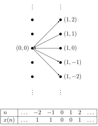
Proof. Givenx∈2Z, we construct a tournament,Tx, with vertices in
Z×Zas follows. Given two vertices at positions (m, n) and (m0, n0) where m, n, m0, n0 ∈ Z, we define
(m, n)→(m0, n0)⇔
m=m0 and n > n0 or
m0 =m+ 1 and x(n0−n) = 1 or |m−m0| ≥2 and m < m0
where, otherwise, there is an edge (m0, n0)→ (m, n). An example of this can be seen in the figure below, where we focus on a pair of columns which are “one apart”. Note thatxis bi-infinite, but for illustration purposes we highlight five consecutive terms inx and the five corresponding vertices in relation to vertex (0,0).
.. .
(0,0)
.. .
.. .
(1,2) (1,1) (1,0) (1,−1) (1,−2) ..
.
n . . . −2 −1 0 1 2 . . .
x(n) . . . 1 1 0 0 1 . . .
Figure 4.1: Directed edges from vertex (0,0) to vertices one column to the right.
Now that we have developed the construction of Tx given x, the aim is to show that there exists a comeager subsetC ⊆2Z, which will be defined later, such that, for
all sequences x, x0 ∈ C,
xEZx0 ⇔Tx∼=Tx0.
To begin, suppose that xEZx0. That is, there exists some k ∈ Z such that, for every n ∈ Z, x(n) = x0(n+k). Now, construct two vertex-transitive tournaments,
Tx and Tx0, from x and x0 respectively as described above. In order to see that Tx and Tx0 are isomorphic, choose any column inTx and similarly forTx0. We claim that
ϕ(m, n) = (m, n+km) is an isomorphism between Tx and Tx0.
we certainly have that ϕis bijective. Further, we notice that adjacency of vertices is preserved as, if (m, n)→(m0, n0) inTxthen we claim that (m, n+km)→(m0, n0+km0) inTx0. To check this, we refer to the above cases where (m, n)→(m0, n0).
If m = m0 and n > n0 then ϕ(m, n) → ϕ(m0, n0) as m = m0 and so n +km > n0 +km0. If m+ 1 = m0 and x(n0 −n) = 1 then we arrive at the same conclusion as m+ 1 = m0 and x0((n0 +km0)−(n+km)) = x0(n0 −n +k) = x(n0 −n) = 1. Finally, if |m−m0| ≥2 andm < m0 then it still remains thatϕ(m, n)→ϕ(m0, n0) as
ϕleaves m and m0 unchanged. Thus, we are able to conclude that ϕ:Tx →Tx0 is an isomorphism.
For the other direction, consider Tx ∼= Tx0. That is, ϕ : Tx → Tx0 gives an isomorphism as described. To see that xEZx0, we must first see that we can recover
xfromTx. In order to do so, we require thatx have sufficiently many 0 and 1 values. To be precise, we require at least one of the following conditions:
(i) For every n there exists somek < n such thatx(k−n) = 1 and x(k) = 0
(ii) For every n there exists somek such thatx(−k) = 0 and x(k−n) = 0
Note that, excluding the trivial case where w= (−1, n), each of these conditions onxareGδand dense, hence comeager. With these requirements, we now come to the definition of the comeager set C containing all x∈2Z satisfying the above conditions.
By the above conditions, for any vertex v, we can identify the five columns surrounding v which we will denote as Sv. More specifically, Sv is the set of points involved in a three-cycle with v.
To see this, let v = (0,0) and consider a second vertex w. In the case that
the case that w = (−1, n) or w = (1, n), n ∈ Z. On the other hand, if w = (−2, n) or w= (2, n) then condition (ii) ensures that there exists a third vertex u such that
w→u and u→v.
We note that it is impossible for there to be a three-cycle involving two vertices that are more than two columns apart. To see that this is the case, suppose that
v = (0,0) andw= (m, n) for|m| ≥3 and for some n ∈Z. Further, suppose there is a third vertexusuch thatw→u. Ifm ≤ −3 thenw→v and, by assumptionw→u. Thereforewcannot be involved in a three-cycle with v. So now, if we considerm≥3, we certainly have v → w. Since w → u then it must be that m0 ≥ m−1 and so
m0 ≥2. That is, |0−m0|=|m0| ≥2 and sov →u. Once again, we see thatwcannot be involved in a three-cycle with v based on our construction.
Further, we can determine distinct columns within Sv as follows:
(i) Let Cv denote the set of all vertices w∈Sv such thatSw =Sv
(ii) LetC−2,vdenote the set of all verticesw∈Sv such thatv does not arrow anyone in Cw
(iii) Let C2,v denote the set of all vertices w∈Sv such thatv is in C−2,w
(iv) Let C−1,v denote the set of all vertices w ∈ Sv such that w 6∈ C−2,v and every
z ∈C2,v is contained in Sw
(v) Let C1,v denote the set of all vertices w ∈ Sv such that for every z ∈ C−1,v,
w∈C2,z.
have x and x0. Well, as ϕ is an isomorphism between Tx and Tx0, ϕ must map C1,v (a Z-ordered subgraph) in Tx to C1,ϕ(v) in Tx0 in an order preserving way. The only possible map is a shift. That is, the edges from v to vertices in C1,v inTx are a shift of the edges from ϕ(v) to vertices in C1,ϕ(v) in Tx0. Well, as x and x0 were used to define these edges respectively it must be the case thatxis a shift of x0 and soxEZx0
as expected.
Finally, we note that the ∼=V T T is strictly more complex than E0. That is, we recall the existence of a∆1
2 reduction fromEω1 to the isomorphism relation on
vertex-transitive linear orders. As linear orders are tournaments we also get that there is a ∆1
2 reduction fromEω1 to the isomorphism relation on vertex-transitive tournaments.
If it were the case that E0 ∼B∼=V T T then there would exist a Borel reduction from ∼
=V T T toE0. But that would meanEω1 was reducible to E0 which cannot be the case
as E0 and Eω1 are incomparable (refer to the remark following Corollary 3.3 in [7])
REFERENCES
[1] John D. Clemens. Isomorphism of homogeneous structures. Notre Dame Journal of Formal Logic, 50(1):1–22, 2009.
[2] R. Dougherty, S. Jackson, and A. S. Kechris. The structure of hyperfinite Borel equivalence relations. Trans. Amer. Math. Soc., 341(1):193–225, 1994.
[3] Harvey Friedman and Lee Stanley. A Borel reducibility theory for classes of countable structures. J. Symbolic Logic, 54(3):894–914, 1989.
[4] Su Gao. Invariant descriptive set theory, volume 293 of Pure and Applied Mathematics (Boca Raton). CRC Press, Boca Raton, FL, 2009.
[5] Joel David Hamkins and Andy Lewis. Infinite time Turing machines. J. Symbolic Logic, 65(2):567–604, 2000.
[6] L. A. Harrington, A. S. Kechris, and A. Louveau. A Glimm-Effros dichotomy for Borel equivalence relations. J. Amer. Math. Soc., 3(4):903–928, 1990.
[7] Greg Hjorth. An absoluteness principle for Borel sets. J. Symbolic Logic, 63(2):663–693, 1998.


![Figure 2.2: Graph of M as constructed by Mekler, [8]](https://thumb-us.123doks.com/thumbv2/123dok_us/8920443.1841227/19.612.253.401.174.264/figure-graph-m-constructed-mekler.webp)