The author wishes to express gratitude to Francesca for her valuable advice and direction with this thesis. The author also wishes to thank Vijay for introducing the author to the area of research. Finally, thanks to the authors of one-pass algo-rithm [35] for sharing the implementation ofgIndex,FG-Index, and their algorithm.
Graph is a commonly used data structure for modeling complex data such as chemical molecules, images, social networks, and XML documents. This complex data is stored using a set of graphs, known as graph database D. To speed up query answering on graph databases, indexes are commonly used. State-of-the-art graph database indexes do not adapt or scale well to dynamic graph database use; they are static, and their ability to prune possible search responses to meet user needs worsens over time as databases change and grow. Users can re-mine indexes to gain some improvement, but it is time consuming. Users must also tune numerous parameters on an ongoing basis to optimize performance and can inadvertently worsen the query response time if they do not choose parameters wisely. Recently, aone-pass algorithm has been developed to enhance the performance of these indexes in part by using the algorithm to update them regularly. However, there are some drawbacks, most notably the need to make updates as the query workload changes.
We propose a new index based on graph-coarsening to speed up query answering time in dynamic graph databases. Our index is parameter-free, query-independent, scalable, small enough to store in the main memory, and is simpler and less costly to maintain for database updates.
We conducted an extensive sets of experiments on two types of databases, i.e., chemical and social network databases, to compare our graph-coarsening based index vs. hybrid-indexes as follows. First, we considered no database updates or query work-load changes (static graph databases) and compared the indexes according to query
indexes in the case of dynamic graph databases, i.e. when graphs are added to or removed from the database. Third, we compared the indexes with regard to query workload changes. Fourth, we studied the scalability of our index vs. hybrid-indexes. Experimental results show that our index outperformshybrid-indexes (i.e. indexes updated with one-pass) for query answering time in the case of social network databases, and is comparable with these indexes for frequent and infrequent queries on chemical databases. Our graph-coarsening index can be updated up to 60 times faster in comparison to one-passon dynamic graph databases. Moreover, our index is independent of the query workload for index update and is up to 15 times better afterhybrid indexes are attuned to query workload for social network databases.
This work is also published in 26th ACM International Conference on Information and Knowledge Management (CIKM) held in Singapore[18].
ABSTRACT . . . vi
LIST OF TABLES . . . xi
LIST OF FIGURES . . . xii
LIST OF ABBREVIATIONS . . . xiv
LIST OF SYMBOLS . . . xv
1 Introduction . . . 1
2 Preliminary Definitions . . . 5
3 Related Work . . . 8
3.1 GIndex . . . 9
3.2 FG-Index . . . 11
3.3 One-pass Algorithm . . . 13
3.4 Discussion . . . 15
4 Graph Database Querying Framework . . . 17
4.1 Graph Coarsening . . . 17
4.1.1 Algorithm . . . 21
4.1.2 Complexity Analysis . . . 22
5 Graph-Coarsening based Index . . . 25
5.1 Query Processing . . . 27
5.2 Index Update . . . 29
5.3 Other Indexing Approaches . . . 30
5.3.1 Graph Reduction Using Query Before Verification . . . 30
5.3.2 Subgraphs And Their Counts . . . 31
6 Experiments and Results . . . 34
6.1 Experiment Setup . . . 34
6.2 Our index vs. hybrid-indexes . . . 37
6.2.1 Social Network Databases . . . 38
6.2.2 Chemical Database . . . 41
6.2.3 Discussion . . . 44
6.3 Comparison on Dynamic Graph Databases . . . 45
6.4 Query Workload Changes . . . 46
6.5 Scalability . . . 48
6.6 Results Summary . . . 49
7 Conclusions . . . 56
7.1 What have we done so far? . . . 56
7.2 Future directions . . . 56
REFERENCES . . . 58
A Reproducing Experiments . . . 62
A.2 Data Formats . . . 62
A.2.1 Generic Graph Format . . . 62
A.3 Running The Code . . . 63
A.3.1 Repository Structure . . . 63
A.3.2 File Naming Convention . . . 64
A.3.3 Chemical Dataset Conversion . . . 65
A.3.4 Labelling Graphs for Social Networks . . . 65
A.3.5 Generating Databases And Queries . . . 66
A.3.6 Experiments . . . 66
A.3.7 Compile And Run . . . 66
5.1 Runtime Comparison with and without Graph Reduction Using Query oneMolecules for different query types . . . 31 5.2 Query Processing Time Comparison with and without subgraph Count 33
6.1 Count of index features on Social Network Databases for Standalone Index comparison . . . 38 6.2 Count of index features on Chemical Database for Standalone Index
comparison . . . 44
3.1 Sample graph database . . . 9
4.1 Example showing chemical compounds as labeled graphs . . . 18
4.2 Examples showing coarnening of graphs . . . 21
5.1 A sample graph databaseD. . . 26
5.2 Graph-coarsening based index example . . . 27
5.3 A sample graph Query Q and its coarsening . . . 28
6.1 Runtime comparison for Frequent queries on Social Network databases. 39 6.2 Runtime comparison for Infrequent queries on Social Network databases. 39 6.3 Runtime comparison for Random queries on Social Network databases. 40 6.4 Index memory consumption comparison for Social Network databases. . 40
6.5 Runtime comparison for Frequent queries on eMolecules database. . . 41
6.6 Runtime comparison for Infrequent queries on eMolecules database. . . . 42
6.7 Runtime comparison for Random queries on eMolecules database. . . 42
6.8 Index memory consumption comparison for eMolecules databases. . . 43
6.9 Database change comparison . . . 45
6.10 Runtime comparison for query workload change for DBLP. . . 50
6.11 Runtime comparison for query workload change for eMolecules. . . 51
6.12 Runtime comparison for query workload change for BlogCatalog3. . . . 52
minSup – Minimum support of a graph in a graph database
XML – Extensible Markup Language
NP– Non-polynomial
maxL – Maximum length or size of a graph
δ-TCFG –delta-Tolerance Closed Frequent subgraphs
GA – Graph Array
IGI – Inverted Graph Index
GHz– Giga-Hertz
MB – Megabyte
GB – Gigabyte
RAM – Random Access Memory
D Graph database
Q Query graph
G Graph
V Set of vertices E Set of Edges
VL Set of Vertex Labels EL Set of Edge Labels
σ Support of a graph in a graph database δ Frequency tolerance factor used in FG-Index DG Set of graphs that contain G
α Swapping parameter used in one-pass ⊆ Subset or equal to
⊂ Subset
6⊆ Not subset or equal to ⊇ Super-set or equal to ∈ Element of
ν A function to assign labels to vertices
≥ Greater or equal γ Discriminative ratio ∩ Set intersection \ Set difference > Greater than
r(B) Coarsening Ratio of a set of edges B
ω(e) Edge-weighting function to compute edge count of edge e ρ(e) Edge-weighting function to compute coarsening ratio of edgee I Coarsening Index
≤ Less than or equal to
CoT Time Complexity of Coarsening SoT Space Complexity of Coarsening
CHAPTER 1
INTRODUCTION
Scientists and practitioners commonly use graphs to model social networks, financial transaction networks, chemical compounds, proteins, images, XML documents or other complex data, and typically store them in graph databases [2, 5, 7, 8, 14, 16, 23, 25, 27, 31, 32, 35]. A graph database D is simply a collection of graphs. A dynamic graph database is a database that changes over time. However, graph databases do not always respond quickly to a user, especially when frequently updated.
by completing a subgraph isomorphism test on every candidate to ensure the query is contained. Optimally, index size fits in main memory, improving query response time.
The research literature identifies many ways to generate features for indexing. The main approaches rely onfrequent subgraphs,paths, ortrees, with varying performance results (see [19] for a survey and performances comparison). However, these indexes do not adapt or scale well to dynamic graph database use; they are static, and as databases change and grow, the indexes become large and outdated, and their ability to reduce the size of a candidate answer set (pruning power) worsens over time [35]. Recently, Yuan et al. [35] proposed aone-passalgorithm to solve this problem by building a starting index with gIndexorFG-Indexand performing updates based on changes to the graph database and query workload (hybrid-index). More specifically, this algorithm keeps the initial number of features constant, and uses the query workload to determine which index features are relevant to the current workload; features more relevant to the current search swap out those that are less relevant. However, this approach assumes that the query workload does not change rapidly. If users do not update the index when query workload starts to change, the query function may not prune a sufficient number of graphs from the search and therefore take longer to deliver results. In real-world applications, databases and queries often change frequently, which would result in the need for frequent index updates. However, attuning the index to the current query workload ignores possible new queries in the future. Consequently, the index will be unable to efficiently answer the full query range. The pruning power for queries not belonging to the query workload used to tune the index will be reduced.
many parameters. While parameters help to reduce the search scope and improve index pruning power, they can do the opposite if not chosen wisely. Research results from several studies illustrate this by showing how their indexes outperform the competition based on the parameter values chosen [7, 19, 32, 35].
We develop a new graph-coarsening based index for graph databases that scales far more effectively todynamic real-world graph database use. Graph coarsening [17] is used to find a more succinct representation of a graph by grouping its vertices together. It preserves basic graph information such as nodes, edges, labels, edge counts, and graph’s sub-structures. Since several nodes and edges in the graph database are frequent, index size remains small and can be stored in the main memory. Also, a coarsened graph is easier to index as the information contained in it can be represented by a simple hashmap.
Therefore, we propose a new index that uses a new definition of graph coarsening to generate an index that is parameter-free, query-independent, scalable and small enough to be stored in main memory which also performs efficient update operations without reducing the pruning power of the index.
We conduct a detailed experimental comparison of our index vs. state-of-the-art solutions fordynamic graph databases on several real-world databases. Experimental results show that: (1) we outperformhybrid-indexes for dynamic graph databases for query answering time by up to 3 times in the case of social network databases. (2) We are scalable with a faster construction time and smaller index size. (3) We can update our index up to 60 times faster in comparison to one-pass. (4) Our index is independent of the query workload for index update and is up to 15 times better afterhybrid-indexes are attuned to query workload.
CHAPTER 2
PRELIMINARY DEFINITIONS
In this chapter, we introduce all the definitions we will use.
Let V L be a set of vertex labels and EL be a set of edge labels. A labeled graph is a 3-tuple G= (V, E, ν) where
• V is the set of vertices,
• E ⊆V ×V ×EL is a set of labeled directed edges, and • ν :V →V L is a function assigning labels to vertices.
We assume labeled graphs to be directed. Whenever we refer to an undirected
graph, we assume each undirected edge (u, v, `) to be represented by both (u, v, `) and
(v, u, `) directed edges.
We define the size of a graph G= (V, E, ν) as |E|.
A graph database D = {G1, G2, ..., Gn} is a set of labeled graphs. Each graph Gi ∈D, i∈[1, n], has a unique identifier denoted by id(Gi).
LetG= (V, E, ν) be a labeled graph and letube a node inV. Thedegree of node
u w.r.t. edge label `, and destination node v’s label ν(v), denoted bydeg(u, `, ν(v)), is defined as the size of the set {v0|(u, v0, `)∈E∧ν(v0) =ν(v)}.
in a graph database. A subgraph query may be contained by graphs in D while a supergraph query may contain graphs in D.
We work with subgraph queries only in this thesis. Graph querying requires us to understand subgraph isomorphism, which is defined as follows.
Definition 2 (Subgraph Isomorphism). Let G = (V, E, ν) and G0 = (V0, E0, ν0) be two labeled graphs. A subgraph isomorphism is an injective function f :V →V0 such that
1. ∀u∈V, ν(u) = ν0(f(u)), and
2. ∀(u, v, `)∈E, (f(u), f(v), `)∈E0.
A graph G is asubgraph of another graph G0, denoted by G⊆ G0, if there exists a subgraph isomorphism from G toG0. Conversely, G0 is called a supergraph of G.
The problem of deciding whether G⊆G0 is called subgraph isomorphism problem and it is proven to be NP-complete [9].
The following definition defines the answer to a graph queryQin a graph database.
Definition 3 (Subgraph Query Processing).
Given a graph database D ={G1, G2, . . . , Gn} and a graph queryQ, the answer to Q
w.r.t. D is the set
ans(Q) ={G∈ D | Q⊆G}
F as a key to the IDs of database graphs that contain the requested feature as a value. The index enables users to retrieve a candidate answer set that filters out false positive candidates. False positive candidates are filtered out by using the following sufficient condition, called inclusive logic. Let F be an index feature, let G∈Dbe a database graph, and letQ be a graph query. If F ⊆Q∧F 6⊆G, then Q6⊆G.
The pruning power of a graph database index is the ability to reduce the size of a candidate answer set.
Given a graph database D ={G1, G2, . . . , Gn} and a graph G, we denote by DG
the set of graphs in the database that contains G. The size of the set DG is called
the support of Gand is denoted by supp(G).
Definition 4(Frequent subgraphs). LetGbe a graph andD={G1, G2, . . . , Gn} be a
graph database. We say that G is a frequent subgraph if supp(G)≥ minSup, where
minSup is a given minimum support threshold.
Definition 5 (Infrequent subgraphs). Let Gbe a graph andD={G1, G2, . . . , Gn} be
CHAPTER 3
RELATED WORK
There are various ways of generating features for indexing graph databases. According to [19], the main approaches rely on (1)simple paths[4, 10, 13, 40], (2)trees[15, 26, 37], (3) graphs [7, 29, 30, 32, 34, 38], and (4) a combination oftrees and graphs/cycles [20]. Among the works that use graphs as features, there are some that rely on frequent subgraphs [7, 32, 38]. Recently, Katsarou et al. [19] compared the performances of CT-index [20], GCode [40], gIndex [32], GRAPES [13], GraphGrepSX [4], and Tree+∆ [38] according to query processing time, index size and index construction time, and scalability. Their experimental results show that GRAPES and Graph-GrepSX are the state-of-the-art best performing indexes for graph databases. How-ever, their comparison is based on static graph databases only and they did not consider, in their analysis, the case of a database changing over time. When the graph database has significantly changed over time, the index becomes outdated and need to be updated. This operation is time consuming and memory intensive [19, 35]. Even if it has been shown that approaches based on frequent graphs such as gIndex and FG-Index are usually an order of magnitude slower than Grapes and Graph-GrepSX on static databases [19], they are, currently, the only ones that can work with
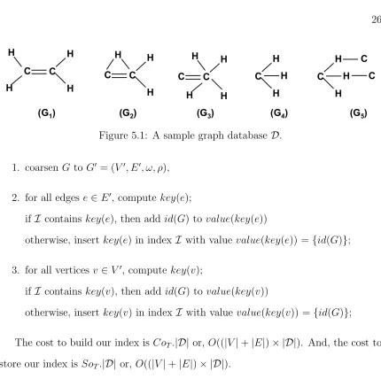
Figure 3.1: A sample graph database [32].
graph databases, we will compare our approach with hybrid-indexes only.
In the following, we give an overview of the above mentioned indexes gIndex and FG-Index, and index update algorithm, one-pass.
3.1
GIndex
gIndex [32] introduced the feature-based indexing approach by first mining a set of features or subgraphs F from graph database D and then, building a map of feature F ∈ F to the set of graph IDs DF that contain F. To mine frequent subgraphs,
the authors used gSpan [31], a depth-first search (DFS) based algorithm. gSpan uses minimum DFS code and lexicographic order to traverse the graph database and reduce isomorphic subgraphs generated from depth-first search traversal up to size
maxL.
The number of fragments, or subgraphs, generated from gSpan varies based on minimum support, minSup. To ensure all queries can be answered, gIndex indexes size-0 (nodes) and size-1 (edges) fragments. Asize-increasing support function is used to reduce the number of fragments generated as the size of fragments increases. There are still many fragments that do not add to the filtering power of the index and are called redundant fragments.
carbon-chains: C, C—C, C—C—C, and C—C—C—C. Fragments C—C, C—C—C, and
C—C—C—C do not provide more indexing power than fragment c. Thus, they are
redundant for indexing. However, the carbon ring in Figure 3.1 is a discriminative
fragment as only graph (c) contains it while graphs (b) and (c) have all of its
sub-graphs. [32]
Therefore, a feature selection is performed to select discriminative fragments that add to the filtering power of the index. These features have support that is much less than the common support between their subgraphs. To identify a discriminative fragment, γ is introduced as the discriminative ratio for a fragment.
Definition 6 (Discriminative Fragment). A frequent subgraph F is discriminative if and only if
| \
F0⊂F,F0∈F
DF0| / |DF|> γ
where γ is the discriminative ratio.
Index is constructed by hashing each discriminative fragment and building a key-value pair of fragment hash as the key and list of graph IDs as the key-value. Once the index is constructed, a query Q can be answered by generating a candidate answer set from the index featuresF by intersecting the graph IDs of features F ∈ F which are subset of Q. More formally, the candidate answer set is defined as
CQ =
\
F⊆Q∧F∈F
DF
3.2
FG-Index
The approach used by FG-Index [7] eliminates candidate verification for frequent subgraphs. Let us suppose that an index uses as features the set of all frequent subgraphs. If a query Q is a frequent subgraph, then verification can be avoided as all the graphs containing the query are the values corresponding to the index feature Q. However, the number of all frequent subgraphs may be big and may cause the index not to fit in the main memory. A way to compress (without loosing any information) the set of frequent graphs is to use the notion of Closed Frequent subgraphs (CFGs).
Definition 7 (Closed Frequent subgraph). A frequent subgraph G is closed if there does not exist another frequent subgraph G0 such that G⊂G0 and DG=DG0.
If the set of features indexed is the set of all CFGs , the answer set of query Q corresponds to
ans(Q) = \
Q⊆F∧F∈F
DF
As a result, time required to answer frequent queries is the same as generating candidate answer set.
The goal of FG-Index is to find a smart way to index all CFGs, as their size may still be too big. Thus, they rely on a relaxed notion of CFGs, namely δ-Tolerance Closed Frequent subgraphs (δ-TCFGs).
Definition 8. (δ-Tolerance Closed Frequent subgraph (δ-TCFG)). A
frequent subgraph G isδ-TCFG if and only if G is a frequent subgraph and there does
not exist another frequent subgraph G0 such that G ⊂ G0 and |DG0| ≥ (1−δ)|DG|,
Usingδ-TCFGs allows us to cluster frequent graphs and generate indexing features for FG-Index which fit in the main memory.
To construct FG-Index, the set of frequent subgraphsFG is mined from the graph
database for a given support minSup. Each graph in FG is assigned with a unique
ID. Then, given a specific value ofδ, the setT ofδ-TCFGs is computed fromFG. The
graphs in T are then sorted by increasing size, decreasing frequency, and increasing unique IDs assigned before. These δ-TCFGs are then stored in main memory in a list called Graph Array (GA) and the list index for each δ-TCFG is used as new ID for graphs in T.
An Edge Array (EA) stores distinct edges from graphs in T. Each edge e in EA further groups graphs inT by the size of the graphs and count ofein each graph, and maps it to id of such graphs in GA. This is called the Inverted-Graph Index (IGI). The first level of IGI is built on T. The next level of IGI is constructed from the set of frequent supergraphs corresponding to a δ-TCFG and each IGI stored on the disk. An Egde-index is included which contains the set of infrequent distinct edges in graph database to ensure any query can be answered.
To answer a query Q, group the query by its distinct edges and get edge counts. For each edgeeinQ, use frequency ofe and findids from Edge Array that have edge count greater than or equal to frequency of e. The intersection of such ids for all edges in Q will give an id. Use this id to get the δ-TCFG G from Graph Array. If G=Q, the answer is DG. Otherwise, useG’s IGI stored on the disk to search forQ.
3.3
One-pass Algorithm
Index construction is done only once to buildgIndex andFG-Index. When the graph database has significantly changed over time, the index features become outdated and need to be re-mined. This operation is time consuming and memory intensive [35]. The one-passalgorithm offers a way to maintain these indexes by applying updates to them. Updates are applied by measuring the goodness of index features known as pruning power. For a query Q, an index feature F ⊆ Q prunes graphs in D \ DF.
More formally:
Definition 9 (Pruning Power and Cover). The pruning power of a feature F is the cardinality ofF’s pruning cover defined asC(F,D,Q) ={(G, Q)|G∈ Dis filtered out by feature F for Q∈ Q}, where D is the graph database and Q is a set of queries to be answered and called query workload.
The pruning cover of the set of index features F is defined as C(F,D,Q) =
S
F∈FC(F,D,Q).
When D and Qare clear from the context, C(F,D,Q) is abbreviated as C(F). Given a starting index, e.g. gIndex or FG-Index, one-pass computes the loss score of each feature in the index and the benefit score of each frequent subgraph which can be added to the index as a feature. The loss and benefit scores are defined in the following.
Definition 11 (Benefit Score). The benefit score B(H,F) of a subgraph H is the increase of the pruning caused by adding H to the set of index features F and it is given by B(H,F) = |C(H)\C(F)|.
When the benefit of adding a frequent subgraphHoutweighs the loss of an indexed featureF, H then replacesF in the index. A swapping criterion, calledswapα, helps
in this decision making by using the loss and benefit scores defined as follows.
Definition 12 (Swapping Criterion (swapα)). An index feature F is replaced by
one-pass algorithm with a frequent subgraph H if
B(H,F)>(1 +α)L(F,F) + (1−alpha)|C(F)|/k
where k is the number of index features and α∈[0,1].
In practice, the value of|C(F)|/kis two orders of magnitude larger thanL(F,F). WhenL(F,F) = 0, a frequent subgraphH with low benefit score will not be swapped in the index. Therefore, 1−α acts as a normalizing factor and, by setting the value of α between 0.95 and 0.995, |C(F)|/k does not dominate the swapping criterion.
Query workload plays an important role in determining the pruning power of the index. When the pruning power drops below a threshold, an update is triggered to swap features. After the updates have been applied, the pruning power of the index is restored for the current query workload. The algorithm keeps the index size near constant since features can only be swapped in and out of the index.
index outperforms the greedy solution defined in [35] to generate an initial index for one-pass algorithm. Therefore, we focus only on the hybrid index to compare with one-pass algorithm.
3.4
Discussion
In this section, we discuss possible drawbacks of the work described above.
Tuning the Index. Features are selected and/or updated based on criteria which utilize different parameters. gIndex uses size-increasing support function and discriminative ratio. FG-Index uses δ and minimum support. One-pass algorithm uses minimum support and α used in swapping criterion. While the parameters help reduce the size and improve pruning power of the index, they can do the opposite if not chosen wisely. Results from [7, 32, 35] show that their indexes outperform the competitors for the parameter values chosen. Further analysis showed gIndex outperformed others for the same parameter values only in the case of sparse graphs andFG-Indexfor only dense graphs [14]. More analysis is required case by case to be able to tune the indexes which enablesgIndex to perform optimally for dense graphs and FG-Index for sparse graphs.
features to be swapped. SincegIndex and FG-Index are not scalable, reconstructing the index can be very time consuming and the size may not fit in the main memory.
CHAPTER 4
GRAPH DATABASE QUERYING FRAMEWORK
In this section, we describe our framework to query evolving graph databases. The framework takes advantage of graph coarsening technique [17] and propose a new definition of graph coarsening suitable for graph database indexing.
4.1
Graph Coarsening
We consider labeled graphs in our graph database. The following example shows how a chemical compound is represented by labeled graph.
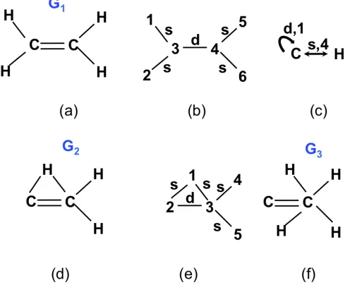
Example 2. Consider the Ethene compound showed in Figure 4.1 (a). We represent
Ethene with a labeled graph G = (V, E, ν) (see Figure 4.1 (b)), where V L={C, H},
EL ={s, d}1, V ={1,2,3,4,5,6}, E = {(1,3, s),(2,3, s), (5,4, s),(6,4, s),(3,4, d)},
ν(1) =ν(2) =ν(5) =ν(6) =H, and ν(3) =ν(4) =C.
Graph-coarsening [17] consists of finding a succinct representation of the graph that also preserves the original graph structure. Usually, a graph G is coarsened by merging together similar vertices into a unique super-node and by assigning edges between super-nodes as follows. If there was an edge between two vertices u and v in G and u has been merged into a new vertex u0 while v has been merged into a new vertex v0, then the coarsened graph G0 will contain an edge between u0 and v0.
Figure 4.1: (a) Ethene compoundG1, (b) Ethene’s representation as a labeled graph,
(c) na¨ıve labeled graph coarsening, (d) and (f) two other compounds G2 andG3, and
(e) G2’s representation as a labeled graph.
Moreover, usually, a weight is added to each edge in the coarsened graph to keep track of the number of edges in the original graph that collapse in a unique edge in the coarsened one. Thus, coarsening is mapping labeled graphs to edge-labeled weighted graphs.
Example 3. Consider the labeled graph representation of the Ethene compound G=
(V, E, ν) from Example 2. Suppose we merge together nodes having the same node
label. A possible coarsening of G is shown in Figure 4.1 (c) and is given by the
edge-labeled weighted graph G0 = (V0, E0, ω) where V0 = {C, H} is the set of nodes,
E0 = {(H, C, s),(C, C, d)} is the set of labeled edges, and ω is the edge weighting
function. Since edges (1,3, s),(2,3, s),(5,4, s), and (6,4, s) from G collapse into the
edge (H, C, s) in G0, we have that ω((H, C, s)) = 4, while ω((C, C, d)) = 1.
the graphs in Figure 4.1 (d) and (f). The coarsening of these two graphs results to be the same of the one of Ethene in Figure 4.1 (a) as they all have four edges between nodesC and H.
Therefore, in order to better preserve the structure of the original graph in its coarsened version, we introduce the concept of coarsening ratio.
Definition 13 (Coarsening ratio). Let G= (V, E, ν) be a labeled graph and let B =
{(u1, v1, `), ...,(un, vn, `)} be the subset of all edges in E such that ν(u1) = ...=ν(un)
and ν(v1) =...=ν(vn). The coarsening ratio r(B)of the set of edges B is defined as
r(B) = 1
max(deg(u1, `, ν(v1)), ..., deg(un, `, ν(v1)))
The coarsening ratio represents the biggest substructure in the original graph involving nodes labeled as ν(u1) and ν(v1), and edge label `.
Example 4. Consider the labeled graph G1 representing Ethene compound in
Fig-ure 4.1 (b). Edges in the set Eb = {(3,1, s), (3,2, s),(4,5, s),(4,6, s)} are all edges
representing a single bond between CarbonCand HydrogenH. We have thatdeg(3, s, H) =
2 and deg(4, s, H) = 2, then, the coarsening ratio for Eb, representing the directed
edge (C, H, s), is r(Eb) = max(21 ,2) = 0.5. On the other hand, Eb0 ={(1,3, s), (2,3, s),
(5,4, s),(6,4, s)} is the set of all the edges having a single bond between Hydrogen H and Carbon C. As deg(1, s, C)) = deg(2, s, C) = deg(5, s, C) = deg(6, s, C) = 1, the coarsening ratio for Eb0, representing the directed edge (H, C, s), is r(Eb0) =
1
max(1,1,1,1) = 1.
Consider now the compound G2 in Figure 4.1 (d). It can be represented as
the labeled graph in Figure 4.1 (e). In this case, the set of edges Ee = {(2,1, s),
(3,1, s),(3,4, s),(3,5,6, s)}, representing a single bond from C to H, has coarsening ratio r(Ee) = max(11 ,3) = 0.33 as deg(2, s, H) = 1 and deg(3, s, H) = 3. For the set of
edges representing the single bond from H to C, the coarsening ration is 0.5 in G2.
For the compound in Figure 4.1 (f ), the coarsening for the set of edges representing
the single bond from C to H is 0.25, while from H to C it is 1.
As we can see, the coarsening ratio allows to distinguish among different graph
structures.
It is worth noting that the coarsening ratio is always a value in the interval (0,1]∪ {∞}.
In our framework, we coarsen labeled graphs to edge-labeled double-weighted2 graphs. Specifically, the edge weighting function ω keeps track of the number of collapsing edges, while the edge weighting function ρ assigns the coarsening ratio to each edge in the coarsened graph.
Definition 14 (Coarsening). Let G = (V, E, ν) be a labeled graph. A coarsening of G is an edge-labeled double-weighted graph G0 = (V0, E0, ω, ρ) such that:
• V0 = {ν(u)|u ∈ V}, i.e. we merge in a unique vertex all vertices in G having the same vertex label (as a consequence, we have |V0| ≤ |V|),
• E0 ={(ν(u), ν(v), ep)|(u, v, ep)∈E},
• ω :E0 →Z≥0 is an edge weighting function s.t. for each edge e = (u0, v0, ep)∈
E0, ω(e) =|A(u0, v0, ep)|, where A(u0, v0, ep) ={(u, v, ep)∈E|u∈ν−1(u0)∧v ∈ ν−1(v0)}, and
Figure 4.2: (a) (resp. (b), (c)) coarsening of graphG1 (resp. G2,G3) from Figure 4.1
according to Definition 14.
• ρ:E0 →(0,1] is an edge weighting function s.t. for each edge e= (u0, v0, ep)∈
E0, ρ(e) =r(A(u0, v0, ep)).
Example 5. Consider graphs G1, G2, and G3 from Figure 4.1. The coarsening of
labeled graphs representing G1, G2, and G3 is shown in Figure 4.2 (a),(b), and (c),
respectively.
The main differences between Definition 14 and the graph coarsening proposed in [17] are the introduction of the coarsening ratio and the absence of a contraction factor regulating the number of nodes in the coarsening (hence we are parameter-free).
4.1.1 Algorithm
Algorithm 1 Graph Coarsening
Input: Graph G= (V, E, ν)
Output: Coarsening C 1: LetC be a hashmap 2: Letdeg be a hashmap 3: for u∈V do
4: if ν(u)6∈C then
5: LetC[ν(u)] be a hashmap
6: for e= (u, v, `)∈ {e0 ∈E|e0 = (u, w, `0)} do
7: if (u, `, ν(v))6∈deg then
8: deg[(u, `, ν(v))]←0
9: Increment deg[(u, `, ν(v))] by 1
10: C[ν(u)][ ][ ]←(0,∞) (for completeness)
11: for key = (u, `, ν(v)) ∈ deg do
12: if ν(v)6∈C[ν(u)]then
13: LetC[ν(u)][ν(v)] be a hashmap 14: if `6∈C[ν(u)][ν(v)]then
15: C[ν(u)][ν(v)][`]←(0,∞) 16: r = 1/deg[key]
17: if r < C[ν(u)][ν(v)][`][1] then
18: C[ν(u)][ν(v)][`][1]←r (coarsening ratio)
19: Increment C[ν(u)][ν(v)][`][0] by deg[key] (edge count)
4.1.2 Complexity Analysis
The time complexity CoT of coarsening is O(|V|+|E|). The coarsening algorithm
iterates through each node and edge only once. The space complexity SoT of
coars-ening isO(|V|+|E|) as most space will be utilized when a graph contains edges with distinct labels for nodes and edges.
4.1.3 Coarsening and Graph Containment
edge count (function ω) to give sufficient conditions to determine if a labeled graph is not contained in another one.
Proposition 1 (Graph containment). Let G1 and G2 be two labeled graphs and let
G01 = (V1, E1, ω1, ρ1) (resp. G02 = (V2, E2, ω2, ρ2)) be the coarsening of G1 (resp.
G2). Let e1 = (u, v, `) ∈ E1 and e2 = (u, v, `) ∈ E2 be two coarsened edges. If
ω1(e1)> ω2(e2) or ρ1(e1)< ρ2(e2) then G1 6⊆G2.
Proof by contradiction. Let us assume that G1 ⊆ G2 and let H1 ⊆ G1 (resp. H2 ⊆
G2) be the subgraph of G1 (resp. G2) such that the coarsening of H1 (resp. H2) is
equal toe1 (resp. e2). SinceG1 ⊆G2, then, by definition of coarsening, alsoH1 ⊆H2.
It follows that, as H1 ⊆H2, we must have that ω1(e1)≤ω2(e2) and ρ1(e1)≥ρ2(e2),
which contradicts the hypothesis.
Example 6. Consider graphs G1, G2, and G3 from Figure 4.1 whose coarsening is
shown in Figure 4.2. According to Proposition 1 we can say that G2 6⊆G1, G2 6⊆G3,
G3 6⊆G1, and G3 6⊆G2.
Consider, for instance, the case G2 6⊆? G1. Let e1 = (C, H, s) be the edge from
C to H in the coarsening G01 = (V10, E10, ω1, ρ1) of G1 (shown in Figure 4.2 (a)) and
let e2 = (C, H, s) be the same edge but in the coarsening G02 = (V20, E20, ω2, ρ2) of
G2 (shown in Figure 4.2 (b)). We have that ρ2(e2) > ρ1(e1) and then, G2 cannot
be contained in G1. The motivation is that G2 contains the features C−H3, i.e. a
Carbon atom connected with three Hydrogen atoms, that in not present in G1 where
the biggest substructure involving C and H is C−H2, i.e. a Carbon atom connected
with two Hydrogen atoms.
that G1 6⊆ G2 because G1 has four different nodes labeled as H, while G2 contains
CHAPTER 5
GRAPH-COARSENING BASED INDEX
The index we propose uses coarsened edges as features instead of frequent subgraphs. A coarsened graph is easier to index as the information contained in it can be represented using a hashmap. Graphs in a coarsened graph database can be grouped by distinct edges, edge weights, and coarsening ratio as the key while graph IDs are stored as the value. Given a coarsened graph G = (V, E, ω, ρ) and an
edge e = (u, v, `) ∈ E, the index key for the edge e is defined as the 5-tuple
key(e) =hu, v, `, ω(e), ρ(e)i. For a graph databaseD, the value, denoted byvalue(e),
for the key key(e) is given by the set of IDs of graphs in D whose coarsening contains the edge e. As we are dealing with edge labeled double-weighted graphs, we refer to the following definition of subgraph isomorphism. Let G = (V, E, ω, ρ) and G0 = (V0, E0, ω0, ρ0) be two edge labeled double-weighted graphs. A subgraph isomorphism is an injective function f : V → V0 such that (1) ∀e = (u, v, `) ∈ E, e0 = (f(u), f(v), `)∈E0, (2) ω(e) =ω0(e0), and ρ(e) = ρ0(e0).
In addition, we also index each single vertex v appearing in a coarsened graph with key key(v) equal to the 5-tuple (v, , ,0,∞) and valuevalue(v) equal to the set of IDs of graphs in D whose coarsening contains the vertex v.
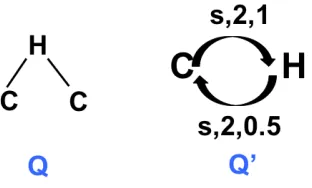
Figure 5.1: A sample graph database D.
1. coarsen G to G0 = (V0, E0, ω, ρ),
2. for all edges e∈E0, compute key(e);
if I contains key(e), then add id(G) to value(key(e))
otherwise, insert key(e) in indexI with value value(key(e)) ={id(G)};
3. for all vertices v ∈V0, compute key(v);
if I contains key(v), then add id(G) to value(key(v))
otherwise, insert key(v) in indexI with value value(key(v)) ={id(G)};
The cost to build our index is CoT.|D| or, O((|V|+|E|)× |D|). And, the cost to
store our index is SoT.|D| or, O((|V|+|E|)× |D|).
Example 7. Consider the graph database in Figure 5.1. The corresponding
graph-coarsening based index I is shown in Figure 5.2.
It is worth noting that our proposed index is parameter-free, as we are not using any parameter to coarsen a graph. Moreover, the size of the index is linear in the size of the graph database, whereas hybrid-indexes index frequent fragments whose size is exponential in the one of the database.
Figure 5.2: Graph-coarsening based indexI for graph databaseDin Figure 5.1. The pair (c, r) denotes the collapsing edge count cand the coarsening ratio r.
graph-coarsening index remains smaller than the database size and can be stored in the main memory. This also enhances the scalability of our index.
5.1
Query Processing
After the graph-coarsening based indexI is constructed for graph databaseD, query processing comprises of (1) generating candidate answer set and (2) candidate verifi-cation.
Candidate answer set CQ for query Q= (V, E, ν) is generated as follows:
1. Coarsen the graph query Q toQ0 = (V0, E0, ω, ρ);
2. Let CQ =D. For each edge e(u, v, `)∈ Q0, intersect CQ with all value sets
Figure 5.3: A sample graph query Q (left) and its coarsening Q0 (right).
I | p≥ω(e)∧q≤ρ(e)}:1
CQ=CQ
\
e(u,v,`)∈E0
\
k∈K
value(k)
3. Remove from CQ all graphs G = (VG, EG, νG) such that there exists a node v ∈VG such that
|{u∈VG|νG(u) =νG(v)}|<|{u0 ∈V|ν(u0) =νG(v)}|
i.e. the graph G does not have enough nodes with label νG(v) to contain the
query Q.
Example 8. Consider the graph databaseDfrom Figure 5.1, the corresponding graph-coarsening based index I shown in Figure 5.2, and the query Q and its coarsening
Q0 = (V0, E0, ω, ρ) from Figure 5.3. E0 contains two edges: e1 = (C, H, s) and e2 =
(H, C, s). By considering edge e1, we have to retrieve from the index I and intersect
all value sets corresponding to the set of keysK1 ={(C, H, s, p, q)∈ I |p≥2∧q≤1}.
Then, we have
CQ0 = \
k∈K1
value(k) ={G1, G2, G3, G4, G5}
The set of database graphs that may contain edge e2 is given, instead, by the
intersection of all value sets corresponding to the set of keys K2 = {(H, C, s, p, q) ∈
I | p≥2∧q≤0.5}, i.e.
CQ00 = \
k∈K2
value(k) ={G2, G5}
Finally, the candidate answer set CQ for query Q is
CQ =CQ0 ∩C
00
Q ={G2, G5}
The cost of query answering is,
CoQueryAnswering =CoCoarsening +CoCandidateGeneration+CQ∗Tsub
=CoT +O(|VQ|+|EQ|) +CQ∗Tsub
=O(|VQ|+|EQ|) +CQ∗Tsub
where, Tsub is the time for subgraph isomorphism test. When no graph is pruned by
the index (worst case), CQ =|D|.
5.2
Index Update
index is query-independent. Conversely, one-pass algorithm needs to update the index even when the query workload is changed.
Adding. When a new graph G is added to graph database, we follow the steps of index construction to add the new graph ID to the graph-coarsening based index I. More specifically, we coarsen G to G0 and, for each edge e in G0, we add the pair hkey(e),{ID(G)}i to index I if key(e) is not present in I, otherwise we add ID(G)
to value(key(e)). A similar index update is done for index entries corresponding to
vertices in G0.
Removing. When a graph G is removed from graph database, its graph ID is removed from all setsvalue(key(e)) where e is an edge in coarsened version G0 of G. Similarly for entries corresponding to vertices in G0. The entry for an edge (and/or vertex) is removed from the index if only graph Gcontained it.
It is worth noting that the cost of updating our index is constant in the size of the graph database, while in the case of hybrid-indexes is inversely correlated to the “quality” of the index before the update [35].
5.3
Other Indexing Approaches
In this section, we describe the additional approaches we had tried. We compared per-formance of the approach described previously with these approaches before deciding to keep it.
5.3.1 Graph Reduction Using Query Before Verification
Once we have a candidate answer setCQwe have to verify whether each graphG∈CQ
the size of subgraph isomorphism test Q ⊆? G, we reduce the size of graph G by
removing from it all nodes v (and edges involving those nodes) such that there does not exist a node v0 in Qwhose label is the same of v’s label.
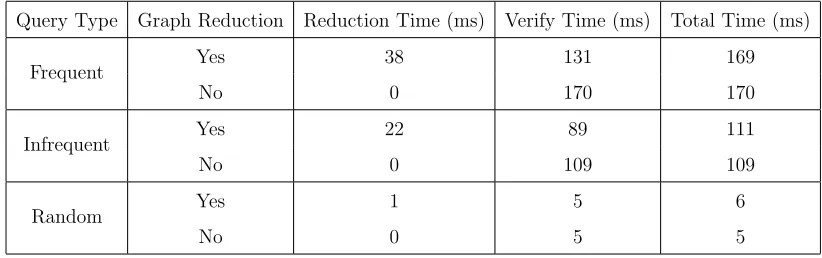
We ran an experiment on eMolecules chemical database to assess improvements of our new approach on different query types, i.e., frequent, infrequent and random (see Section 6.1 for definition). Table 5.1 shows the verification time results for the experiment conducted on chemical database. This approach improved the verification time from 171 ms to 138 ms, for frequent queries, but the reduction time was large enough (38 ms) that there was no noticeable gain in total time taken. Therefore, we decided to keep our original approach.
Table 5.1: Runtime Comparison with and without Graph Reduction Using Query on eMolecules for different query types. Rows with Yes for Graph Reduction in the table use the new approach.
Query Type Graph Reduction Reduction Time (ms) Verify Time (ms) Total Time (ms)
Frequent Yes 38 131 169
No 0 170 170
Infrequent Yes 22 89 111
No 0 109 109
Random Yes 1 5 6
No 0 5 5
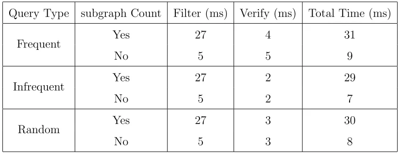
5.3.2 Subgraphs And Their Counts
Consider Figure 4.1, the original index cannot answer that G1 6⊆ G2 and G1 6⊆ G3.
The reason is that there is no information in G1 that is not contained inG2. Let us
consider coarsened edgeC−H in Figure 4.2 (a), (b) that represents coarsening ofG1
the coarsening ratio is also greater forC−H in coarsened G1, when G1 is the query,
causing G2 to not be eliminated.
When we reconsider graphsG1andG2, there is only one subgraph with oneC−H2
inG2 but two of such subgraphs in G1. If we add the count of these subgraphs along
with the coarsening ratio of each subgraph, there is only one subgraph C−H2 inG2
which allows for possibility of only one graph that is one C −H2 in G1. G2 can be
eliminated with this approach. Same applies for G3 as there is only one substructure
with one C and four H.
Table 5.2: Query Processing Time Comparison with and without subgraph Count. Rows with Yes for subgraph Count use the new approach.
Query Type subgraph Count Filter (ms) Verify (ms) Total Time (ms)
Frequent Yes 27 4 31
No 5 5 9
Infrequent Yes 27 2 29
No 5 2 7
Random Yes 27 3 30
CHAPTER 6
EXPERIMENTS AND RESULTS
As reported in Chapter 3, there are many indexes defined for graph databases. However, the majority of them do not adapt in case of database changes.
As the main goal of our work is to provide a solution for dynamic graph databases,
in this section we compare our graph-coarsening index and the state-of-the-art indexes
working for dynamic graph databases, i.e. hybrid-indexes.
6.1
Experiment Setup
We used the implementation ofhybrid-indexes developed for the paper [35] and kindly provided by the authors. Since their implementation was in Java, we used the same language to implement our index. The verification algorithm used is VF2[24].
of the huge size of the network and restrictions on the API. Often, information is gathered for individual nodes, together with their neighbors and neighbors’ neighbors, i.e. ego networks, or with all neighbors up to a fixed distance. It is clear that, in this case, the retrieved data is in the form of a graph database. Also, OSNs are dynamic as they continuously chance over time. Since a social network is a single graph, we computed ego networks from nodes in the social network to generate a graph database. We use three social networks for comparison, namely DBLP [21], BlogCatalog3[36], andSlashdot[21]. Slashdotis a signed network (i.e. it contains two types of relationships, namely friend and foe relationship) while BlogCatalog3 andDBLP are unsigned. The three social networks have 317,080 (MGD=0.77), 10,312 (MGD=0.89) and 77,357 egos (MGD=0.61) respectively. We labeled nodes in the social networks as follows. First, we computed the page-rank of nodes in a network by using the SNAP library [22]; second, we assigned 10 node labels, 0-9, to the nodes of each social network (there are 7 node labels ineMolecules). To assign a label, we computed the page rank of each node, and uniformly distributed the page ranks into 10 buckets between the upper and lower bound of the computed page ranks.
The chemical database is indexed with minimum supports of 10%, 20%, 30% and 40% of the database size. For a fair comparison, we use 2%, 3% and 4% for social networks as there were not many subgraphs at minimum support of 10% or higher. We set the δ= 0.1 to compute δ-TCFGs for FG-Index.
three types of queries we proceeded as follows. We first mined frequent subgraphs with a low minimum support of 1%. To generate frequent queries, we then selected mined subgraphs that have minimum support greater than or equal to the minimum support used to build the index. To generate infrequent queries, we selected subgraphs that have a minimum support less than the one of the index (and greater than 1%). To generate query sets, we randomly sampled a subset of frequent and infrequent queries respectively. We used database graphs to select random queries and generate query sets. Each query set contained 1,000 queries. The size of each graph database used in the experiments is 30,000 graphs. If the number of graphs in the database was less than 30,000 graphs, we randomly chose graphs from the database till we reached 30,000 graphs.
The index construction time for other indexes on ego networks was daunting due to the size of the ego networks. Therefore, we used a maximum graph size of 15 for DBLP and BlogCatalog3 ego networks. The two databases contained sparse graphs. However, ego networks in Slashdot were dense and to construct indexes in a reasonable amount of time we changed the maximum size constraint to 10 edges. The graph database for Slashdot was still dense.
We tested the indexes for 10 sets of 1,000 queries for each query type and averaged the results for each query set and computed the mean of all query sets. If the number of queries was less than 1,000, queries were randomly repeated to reach desired size. The frequent and infrequent queries were mined with gSpan [31] using maxL=10. The index features were also mined with maxL=10.
-FG-Index. Since a majority of time is spent on candidate answer set verification during query processing, the size of the candidate answer set is important to speed-up query answering. Therefore, a faster query answering time suggests a candidate set is closer to the actual answer. We define this closeness asgoodness of candidate answer set.
We conducted four sets of experiments to compare our graph-coarsening based index vs. hybrid-indexes. First, we considered no database updates or query work-load changes (static graph databases) and compared the indexes according to query answering time and index size for different minSup values. Results are reported in Section 6.2. Second, we compared the indexes in the case of dynamic graph databases, i.e. when graphs are added to or removed from the database. Results are reported in Section 6.3. Third, we compared the indexes with regard to query workload changes. Results are shown in Section 6.4. Finally, we studied the scalability of our index vs. hybrid-indexes. Results are shown in Section 6.5.
6.2
Our index vs. hybrid-indexes
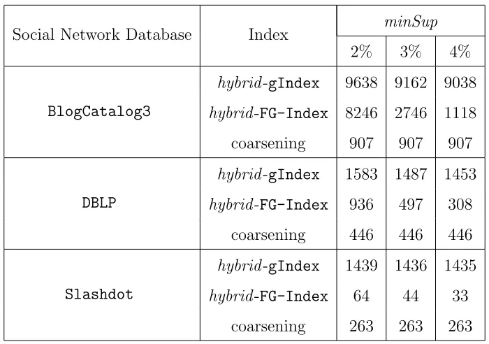
Table 6.1: Count of index features on Social Network Databases for Standalone Index comparison
Social Network Database Index minSup
2% 3% 4%
BlogCatalog3
hybrid-gIndex 9638 9162 9038 hybrid-FG-Index 8246 2746 1118 coarsening 907 907 907
DBLP
hybrid-gIndex 1583 1487 1453 hybrid-FG-Index 936 497 308
coarsening 446 446 446
Slashdot
hybrid-gIndex 1439 1436 1435 hybrid-FG-Index 64 44 33
coarsening 263 263 263
6.2.1 Social Network Databases
The run time on social network databases of our graph-coarsening index vs. hybrid -indexes for different minimum supports is shown in Figures 6.1, 6.2 and 6.3 for answering frequent, infrequent, and random queries, respectively. Table 6.1 shows the number of features indexed for differentminSup values by database. The number of features for FG-Index are reported for what was stored in main memory and on disk.
Figure 6.1: Runtime comparison for Frequent queries on Social Network databases.
Figure 6.2: Runtime comparison for Infrequent queries on Social Network databases.
per feature is lower however.
Figure 6.3: Runtime comparison for Random queries on Social Network databases.
Figure 6.4: Index memory consumption comparison for Social Network databases.
index has a higher quality of features.
For Slashdot database, we observe a different pattern. Our index performs comparably to both hybrid-gIndex and hybrid-FG-Index for frequent queries, but outperforms them for infrequent and random queries. This shows our index performs well for dense databases as well.
type (and min support as well) and we are always able to answer any query in less than 20 ms for social network databases.
The comparison of memory consumption between our graph-coarsening index and hybrid-indexes for different minimum supports is shown in Figure 6.4 for social network databases. We require up to 4 times less space compared to hybrid-gIndex while up to 10 time less space compared tohybrid-FG-Index(seeBlogCatalog3 min-Sup=2%). Lesser number of index features in Table 6.1 also supports that our index
requires less memory. Higher memory consumption in case of hybrid-FG-Index with less features is due to index stored on disk compared to our index or hybrid-gIndex which are stored in main memory only.
Figure 6.5: Runtime comparison for Frequent queries on eMolecules database.
6.2.2 Chemical Database
Figure 6.6: Runtime comparison for Infrequent queries on eMolecules database.
Figure 6.7: Runtime comparison for Random queries on eMolecules database.
features for hybrid-FG-Index are reported for what was stored in main memory and on disk.
Figure 6.8: Index memory consumption comparison for eMolecules databases.
verification. But as minSup increases, lesser number of queries is answered directly that requires index feature joins to generate candidate answer sets. Therefore, more subgraph isomorphism tests need to be performed to get the answer. The number of features in our index is less than hybrid-indexes for minSup ≤ 30% but better or comparable performance which shows our index has a higher quality of features.
We beat hybrid-FG-Index at minSup=40% for infrequent queries. And, we are comparable withhybrid-FG-Index for random queries on testing with the same min-imum support.
The size of the candidate set for queries against graph-coarsening index grows as support of the queries decreases. A less frequent coarsened query is contained in a larger set of graphs because the coarsening is more common in the graphs than the structure of the query itself and requires more time for verification. This is why the query answering time is nearly constant across different minimum supports for our index.
Table 6.2: Count of index features on Chemical Database for Standalone Index comparison
Chemical Database Index minSup
10% 20% 30% 40%
eMolecules
hybrid-gIndex 799 596 532 512 hybrid-FG-Index 2619 769 361 229 coarsening 329 329 329 329
hybrid-indexes for different minimum supports is shown in Figure 6.8 for the chemical database. In general, our index uses far less memory than competitors.
We require 4 to 6 times less space compared to hybrid-gIndex while 6 times to 17 times less space compared tohybrid-FG-Indexto store the index when going from 40% minimum support to 10% minimum support. Lesser number of index features in Table 6.2 also supports that our index requires less memory.
6.2.3 Discussion
(a) Query time.
(b) Update time.
Figure 6.9: (a) Runtime comparison for graph DB change between different datasets for frequent queries. (b) Index update time comparison.
6.3
Comparison on Dynamic Graph Databases
in the swapping criterion for updating the hybrid-indexes with one-pass algorithm was set to 0.99.
Figure 6.9 (a) shows the query answering time before and after the index update. We observe thathybrid-indexes benefit from the update made byone-passalgorithm, especially in the case of chemical database. Our index, instead, is up to date at any time and maintains a constant pruning power, independently of the database update. Our index is comparable for social network databases in terms of query processing before and after the update. Regarding the time for updating the index, as shown in Figure 6.9 (b), we are up to 60 times faster thanone-pass algorithm.
6.4
Query Workload Changes
In this section, we compare the querying time when the query workload type changes over time. The one-pass uses query workload changes to detect and update the index. It uses ADWIN [3] for change detection and if the query workload has changed significantly, update is applied to the index. Our index does not depend on query workload and remains current with regards to it. Moreover, we do not have any cost in updating the index as we are query independent.
or random then infrequent. For ease of understanding, the query workload changes we used are as follows.
1. Frequent → Infrequent → Frequent queries
2. Frequent → Random →Frequent queries
3. Frequent → Infrequent → Random→ Frequent queries 4. Frequent → Random →Infrequent → Frequent queries
Change in query workload was detected by ADWIN which triggered index update and features were swapped. While the index was updating, we used the current index until the updated index was available for use. We ranhybrid-indexes withminSup= 2% (resp. 10%) in case of social networks (resp. eMolecules).
Figure 6.10 and 6.11 show the query answering time for this experiment on DBLP and eMolecules, and Figure 6.12 and 6.13 show the query answering time onBlogCatalog3 and Slashdot. The results are plotted using a line graph for each batch of 100 queries and workload change can be noticed as querying time changes for every 10,000 queries. While running the code for hybrid-indexes, the code to update the index threw exception. The runtime after exception is reported as dropping to zero. It is unclear why the code threw exception. Since we were using previous implementation, we did not modify it.
on social network databases and results independent of the query workload. For frequent queries, we are up to 15 times better thanhybrid-FG-Indexand up to 7 times better thanhybrid-gIndex. In the case of chemical database, we are comparable, and sometimes better, than competitors on frequent queries.
6.5
Scalability
In this section, we compare the scalability of our graph-coarsening index withhybrid -indexes. For this experiment, we followed the same approach asone-passpaper [35], i.e., we randomly sample five graph databases from eMolecules database. These databases have a size from 216 to 220 graphs.
Figures 6.14 (a) and (b) show the index construction time and memory usage, re-spectively, for different database sizes. hybrid-indexes were built withminSup=10%. Our graph-coarsening based index is always faster to construct and requires up to 6 (resp. 5) times less space than hybrid-FG-Index (resp. hybrid-gIndex). Results show our index grows linearly space-wise, while other indexes grow exponentially, with increase in database size, making our index desirable for larger databases.
Moreover, we also compare the construction time and memory usage with different minimum supports in the case of a database containing 216 graphs. Results are shown
6.6
Results Summary
In summary, our index outperforms competitors on denser graph databases (e.g. so-cial networks) and performs comparably for sparse ones (e.g. chemical databases).
Experimental results show that:
(1) We outperform state-of-the-art indexes for query answering time by up to 3 times in the case of social network databases. In the case of chemical database, we are comparable with hybrid-indexes for frequent and infrequent queries.
(2) We are scalable with a faster construction time and smaller index size.
(3) We can update our index up to 60 times faster in comparison to one-pass algorithm for dynamic graph databases.
(a) Index construction time for different database sizes.
(b) Memory consumption for different database sizes.
CHAPTER 7
CONCLUSIONS
7.1
What have we done so far?
We proposed a new index based on graph-coarsening for speeding up the query answering time in dynamic graph databases. The index is parameter-free, query-independent, scalable, small enough to store in the main memory, and is simpler and less costly to maintain in case of database updates.
Experimental results showed that we outperformhybrid-indexes for query answer-ing time in the case of social network databases. In the case of chemical database, we are comparable with competitors for frequent and infrequent queries. We can update our index up to 60 times faster in comparison toone-passfor dynamic graph databases. Moreover, our index is independent of the query workload for index update and is up to 15 times better after hybrid-indexes are attuned to query workload.
7.2
Future directions
• Number of nodes • Density
• Number of distinct node labels • Number of graphs in the database
Queries will be generated for each parameter after the database has been created. We will compare the results with state-of-the-artstatic indexes such as GRAPES [19] and GraphGrepSX [4]. We will use GraphGen [1] algorithm to generate synthetic data.
In future, we also plan to use our index to study the following.
• Test our graph-coarsening based index for supergraph search, i.e. when the answer to a queryQis the set of all graph databasesGs.t. Q⊇G, and compare our performances with cIndex [6], the state-of-the-art index for supergraph query and cIndex updated by one-pass.
• Compare performance of our index on a cluster for very large graph databases by exploring ways a database can be distributed over a cluster.
• Study substructure similarity search in graph databases, i.e. finding similar structures in a graph database by edge relaxations on a query graph [33]. Basi-cally, edge relaxation allows node and edge labels to be ignored in a query graph while preserving total edge counts. Our index can adapt to these relaxations and can be used to generate a candidate set.
REFERENCES
[1] Graphgen — a synthetic graph data generator. http://www.cse.ust.hk/ graphgen/.
[2] Stefano Berretti, Alberto Del Bimbo, and Enrico Vicario. Efficient matching and indexing of graph models in content-based retrieval. IEEE Transactions on Pattern Analysis and Machine Intelligence, 23(10):1089–1105, 2001.
[3] Albert Bifet, Geoff Holmes, Bernhard Pfahringer, and Ricard Gavald`a. Mining frequent closed graphs on evolving data streams. InProceedings of the 17th ACM SIGKDD International Conference on Knowledge Discovery and Data Mining, KDD’11, pages 591–599, 2011.
[4] Vincenzo Bonnici, Alfredo Ferro, Rosalba Giugno, Alfredo Pulvirenti, and Den-nis Shasha. Enhancing graph database indexing by suffix tree structure. In Proceedings of the 5th IAPR International Conference on Pattern Recognition in Bioinformatics, PRIB’10, pages 195–203, 2010.
[5] Christian Borgelt and Michael R Berthold. Mining molecular fragments: Finding relevant substructures of molecules. In Proceedings of the 2002 IEEE Interna-tional Conference on Data Mining, ICDM’02, pages 51–58. IEEE, 2002.
[6] Chen Chen, Xifeng Yan, Philip S Yu, Jiawei Han, Dong-Qing Zhang, and Xiaohui Gu. Towards graph containment search and indexing. InProceedings of the 33rd International Conference on Very Large Data Bases, VLDB’07, pages 926–937, 2007.
[7] James Cheng, Yiping Ke, Wilfred Ng, and An Lu. Fg-index: Towards verification-free query processing on graph databases. InProceedings of the 2007 International Conference on Management of Data, SIGMOD’07, pages 857–872, 2007.
[9] Stephen A. Cook. The complexity of theorem-proving procedures. InProceedings of the Third Annual ACM Symposium on Theory of Computing, STOC’71, pages 151–158, 1971.
[10] Raffaele Di Natale, Alfredo Ferro, Rosalba Giugno, Misael Mongiov`ı, Alfredo Pulvirenti, and Dennis Shasha. Sing: Subgraph search in non-homogeneous graphs. BMC bioinformatics, 11(1):96, 2010.
[11] eMolecules Database. http://www.emolecules.com. [12] GitLab. http://www.gitlab.com.
[13] Rosalba Giugno, Vincenzo Bonnici, Nicola Bombieri, Alfredo Pulvirenti, Alfredo Ferro, and Dennis Shasha. Grapes: A software for parallel searching on biological graphs targeting multi-core architectures. PloS one, 8(10):e76911, 2013.
[14] Wook-Shin Han, Jinsoo Lee, Minh-Duc Pham, and Jeffrey Xu Yu. igraph: A framework for comparisons of disk-based graph indexing techniques. Proceedings of the VLDB Endowment, 3(1):449–459, 2010.
[15] Huahai He and Ambuj K Singh. Closure-tree: An index structure for graph queries. InProceedings of the 22nd International Conference on Data Engineer-ing, ICDE’06, pages 38–38, 2006.
[16] CA James, D Weininger, and J Delany. Daylight theory manual daylight version 4.82. daylight chemical information systems, 2003.
[17] Chanhyun Kang, Sarit Kraus, Cristian Molinaro, Francesca Spezzano, and V. S. Subrahmanian. Diffusion centrality: A paradigm to maximize spread in social networks. Artificial Intelligence, 239:70–96, 2016.
[18] Akshay Kansal and Francesca Spezzano. A scalable graph-coarsening based index for dynamic graph databases. In 26th ACM International Conference on Information and Knowledge Management (CIKM), CIKM’17, 2017.
[19] Foteini Katsarou, Nikos Ntarmos, and Peter Triantafillou. Performance and scalability of indexed subgraph query processing methods. Proceedings of the VLDB Endowment, 8(12):1566–1577, 2015.
[20] Karsten Klein, Nils Kriege, and Petra Mutzel. Ct-index: Fingerprint-based graph indexing combining cycles and trees. In Proceedings of the 27th International Conference on Data Engineering, ICDE’11, pages 1115–1126, 2011.
[22] Jure Leskovec and Rok Sosiˇc. Snap: A general-purpose network analysis and graph-mining library. ACM Transactions on Intelligent Systems and Technology (TIST), 8(1):1, 2016.
[23] Thomas Madej, Jean-Fran¸cois Gibrat, and Stephen H Bryant. Threading a database of protein cores. Proteins: Structure, Function, and Bioinformatics, 23(3):356–369, 1995.
[24] Luigi P. Cordella, Pasquale Foggia, Carlo Sansone, and Mario Vento. A (sub)graph isomorphism algorithm for matching large graphs. IEEE Transac-tions on Pattern Analysis and Machine Intelligence, 26(10), 2004.
[25] Euripides G. M. Petrakis and A Faloutsos. Similarity searching in medical image databases. IEEE Transactions on Knowledge and Data Engineering, 9(3):435– 447, 1997.
[26] Haichuan Shang, Ying Zhang, Xuemin Lin, and Jeffrey Xu Yu. Taming ver-ification hardness: An efficient algorithm for testing subgraph isomorphism. Proceedings of the VLDB Endowment, 1(1):364–375, 2008.
[27] Ali Shokoufandeh, Sven J Dickinson, Kaleem Siddiqi, and Steven W Zucker. Indexing using a spectral encoding of topological structure. In Proceedings of the IEEE Computer Society Conference on Computer Vision and Pattern Recognition, volume 2 of CVPR’99, 1999.
[28] SMILES. https://en.wikipedia.org/wiki/Simplified molecular-input line-entry system.
[29] David W Williams, Jun Huan, and Wei Wang. Graph database indexing using structured graph decomposition. In Proceedings of the 23rd International Conference on Data Engineering, ICDE’07, pages 976–985, 2007.
[30] Yan Xie and Philip S Yu. Cp-index: on the efficient indexing of large graphs. In Proceedings of the 20th ACM International Conference on Information and Knowledge Management, CIKM’11, pages 1795–1804, 2011.
[31] Xifeng Yan and Jiawei Han. gspan: Graph-based substructure pattern mining. In Proceedings of the 2002 IEEE International Conference on Data Mining, ICDM’02, pages 721–724, 2002.
[33] Xifeng Yan, Philip S. Yu, and Jiawei Han. Substructure similarity search in graph databases. In Proceedings of the 2005 ACM SIGMOD International Conference on Management of Data, SIGMOD ’05, pages 766–777, 2005.
[34] Dayu Yuan and Prasenjit Mitra. Lindex: a lattice-based index for graph databases. The VLDB Journal, 22(2):229–252, 2013.
[35] Dayu Yuan, Prasenjit Mitra, Huiwen Yu, and C. Lee Giles. Updating graph indices with a one-pass algorithm. In Proceedings of the 2015 International Conference on Management of Data, SIGMOD’15, pages 1903–1916, 2015.
[36] Reza Zafarani and Huan Liu. Social computing data repository at ASU. http://socialcomputing.asu.edu, 2009.
[37] Shijie Zhang, Meng Hu, and Jiong Yang. Treepi: A novel graph indexing method. In Proceedings of the 23rd International Conference on Data Engi-neering, ICDE’07, pages 966–975, 2007.
[38] Peixiang Zhao, Jeffrey Xu Yu, and Philip S. Yu. Graph indexing: Tree + delta >= graph. In Proceedings of the 33rd International Conference on Very Large Data Bases, VLDB ’07, pages 938–949, 2007.
[39] Yuanyuan Zhu, Lu Qin, Jeffrey Xu Yu, and Hong Cheng. Finding top-k similar graphs in graph databases. In Proceedings of the 15th International Conference on Extending Database Technology, EDBT’12, pages 456–467, 2012.
APPENDIX A
REPRODUCING EXPERIMENTS
A.1
Getting the code
The code can be downloaded from GitLab [12] at the URL below. The repository will be made public after publication of this thesis.
URL: https://[email protected]/akshaykansal1/graph-index.git The repository can be cloned and opened in Eclipse. We used Mars to write the code. The code was written in and is compatible with Java SE 7.
A.2
Data Formats
The implementation mainly deals with two formats of graph data. 1. SMILES [28] - Mainly for chemical data from eMolecules. 2. Generic Graph Format
A.2.1 Generic Graph Format
This format was introduced with gSpan [31]. The graph in the example below are undirected.
Example:
and e represents an edge that connects source node idi to destination node idj with labelel.
t # 0 (graph id) v 0 0 (v i l) v 1 0
v 2 0
e 0 1 1 (e i j el) e 1 2 1
e 0 2 1
A.3
Running The Code
This section covers the basic structure of the code base, file naming conventions used, data formatting for social networks and running experiments.
Please Note: All code written in this repository has file names hard coded
A.3.1 Repository Structure
The repository is structured as follows.
1. ./dblp, ./slashdot, ./blogcatalog, ./gindex contain the data used for the experiments.
2. ./lib contains jarneeded to run the code.
![Figure 3.1: A sample graph database [32].](https://thumb-us.123doks.com/thumbv2/123dok_us/8919968.1841022/25.612.200.447.106.170/figure-a-sample-graph-database.webp)