Developing and Testing an Anguilliform Robot Swimming with Theoretically High Hydrodynamic Efficiency

(1)

University of New Orleans University of New Orleans

ScholarWorks@UNO

University of New Orleans Theses and

Dissertations Dissertations and Theses

Fall 12-18-2015

Developing and Testing an Anguilliform Robot Swimming with

Theoretically High Hydrodynamic Efficiency

John B. Potts III

University of New Orleans, [email protected]

Follow this and additional works at: https://scholarworks.uno.edu/td

Part of the Acoustics, Dynamics, and Controls Commons, Computer-Aided Engineering and Design

Commons, Controls and Control Theory Commons, Engineering Physics Commons, Fluid Dynamics Commons, Ocean Engineering Commons, Other Engineering Commons, Other Mechanical Engineering Commons, and the Systems Engineering Commons

Recommended Citation Recommended Citation

Potts, John B. III, "Developing and Testing an Anguilliform Robot Swimming with Theoretically High Hydrodynamic Efficiency" (2015). University of New Orleans Theses and Dissertations. 2103. https://scholarworks.uno.edu/td/2103

(2)

Developing and Testing an Anguilliform Robot Swimming with Theoretically High Hydrodynamic Efficiency

A Dissertation

Submitted to the Graduate Faculty of the University of New Orleans

in partial fulfillment of the requirements for the degree of

Doctor of Philosophy in

Engineering and Applied Science Naval Architecture and Marine Engineering

by

J. Baker Potts, III [email protected] [email protected]

B.S. Tufts University, 2009 M.S. University of New Orleans, 2012

(3)

c

(4)

For my beautiful and lovely wife, Kaity, who never ceased to be patient with me over the past four and a half years yet still motivating me to complete this body of work. Thanks.

“The best time to plant a tree was 20 years ago. The second best time is now.”

— Chinese Proverb

“To know, is to know that you know nothing. That is the meaning of true knowledge.”

(5)

ACKNOWLEDGEMENTS

I am extremely grateful to several individuals and entities for the help over the past few years during the completion of this research. Without these people, I would have never been able to complete such an exhaustive body of work.

The Office of Naval Research, specifically Program Manager Kelly Cooper, awarded funding for the development and experimental analysis of the robotic eel presented within. This funding was awarded through grant number N00014-11-1-0830 to the principal investigator of Dr. Brandon Taravella at UNO’s Department of Naval Architecture and Marine Engineering. A direct result of this award to date has been the completion of two working prototypes and a substantial body of knowledge of practical anguilliform robot design and justification of the theory behind the propulsive wake produced by these robots. If it hadn’t have been for Ms. Cooper’s award, none of this would have been accomplished, so I am very grateful to her.

A separate DURIP grant (# N00014-12-1-0782) was acquired to procure custom PIV (Parti-cle Image Velocimetry) equipment which allowed for the measuring of whole-field velocities in a fluid flow. This equipment significantly increased the experimental testing capabilities of the UNO Towing Tank with a cutting-edge product, aiding it to complete similar work of other top-notch universities. Even with this new measuring device, the experience and knowledge of the profes-sors and staff engineers on the capabilities and constraints of this type of testing has increased immeasurably. This extremely specialized equipment that is able to ride on the UNO Towing Tank carriage, one of a few in the world, was very expensive and would not have been obtained without the DURIP grant.

(6)

I am extremely grateful for this. He is very creative and full of talent. He is the best at bouncing off product development ideas, such as during the development and fabrication of the anguilliform robot prototypes. He is also extremely knowledgeable with electrical engineering, aiding with all the aspects associated with this field, such as the mechatronics and programming. He wrote the LabVIEW program to remotely control the robot prototypes, and this was a difficult and time-consuming undertaking. Ryan helped me countless other times throughout the project on tasks such as experimental testing equipment setup or whenever I encountered a mental stumbling block. UNO NAME Facilities Manager George Morrisey has been very helpful with anything related to equipment in the UNO Towing Tank and Model Shop. If a testing apparatus needed fabrication or help was needed during some testing, he was the person to talk to. At times, George was a good motivator with his can-do attitude. Where I was very thoughtful and planned the project to the smallest details, George would tell me “stop thinking, just do!”

Several undergraduate and graduate students have helped me over the years. Chase Rogers worked on the computational fluid dynamics part of the project and helped me intermittently during tank testing. Chase was also a good person to bounce mathematical and programming ideas off of, as well as being an entertaining person to be around, bringing levity to the graduate student offices. Jacob Todd began the CFD part of the project for Chase and also helped me with various setting up of tests in the tank. Cory Collongues helped with ordering parts from various companies and vendors. Jan Felix, the UNO NAME Department Administrator, also helped with ordering parts from vendors and helped me with submitting the correct paperwork at the right times. Jake Kindred helped me set up the testing of the robot for load cell measurements and PIV testing. Jackson Wilson helped the most out of the research assistants, mostly because of his specialty experience in SCUBA diving. With this capability, he was able to set up the PIV calibration plate underwater, which is a time-consuming process that required more than just breaths of air. Jackson also helped with the fabrication of the tether, creating the CAM toolpath generation and setting up the tooling in the CNC mill.

(7)

technical expertise helped to obtain better results of the robot’s flow field.

I am grateful for the committee members that took the time to go over my dissertation research and meet with me several times for discussion of testing results. Lothar Birk is brilliant and saw the project from angles I never would have imagined. His expertise in fluid dynamics was very instructive. Kazim Akyuzlu was very instructive with the particle image velocimetry equipment, particularly lending out his hot-wire anemometer to verify the PIV measurements. George Ioup is an expert in signal processing and filtering, and he helped me with filtering all of the time-series data without forgetting 2π in the exponent of my Fourier transforms, to say the least. Nikolas Xiros aided me with the control theory aspects of the project, which is a huge undertaking in its own right.

I am grateful for William Vorus coming up with this theory back in the 1990’s. If he had not have seen that snake slithering across a pollen-covered pond, and thus showing off its shed vortex trail, this idea for an ideal anguilliform motion would have never come to fruition. His mathematical genius also enabled this complicated theory to be derived. I know this project means a lot to him, and I am honored to continue on and progress the research of his ideal anguilliform motion.

Brandon Taravella, my dissertation advisor, has obviously been the most helpful over the years, steering me in the right direction, during my lows and highs. His technical expertise in math, dynamics, and fluid dynamics has always been very helpful to rely upon during times of hardship. It has been a pleasure to work with him over the years with his guiding yet backed-off approach. He gave me plenty of space to work on my dissertation research and allowing me to go in the direction I felt it needed to go. I am still honored that he asked me to join him on this project over four years ago. If this had not have happened, I would have been performing typical engineering calculations somewhere. Now, I can say I have worked on one of the coolest projects.

Thank you to my parents, John and Adele, for providing the environment to allow me to get to this stage in my career. They have been so self-less and accommodating, aiding me by limiting the times for me to be stressed out by the mundane demands of life. They cooked countless meals and poured refreshing beers for me to forget the stresses of the day and enjoy some necessary family time.

(8)

During the lowest moments, she reminded me why I was working on this tiring work and motivated me to return to my path of one step at a time. During the highs, she kept me humble and made me not forget what work was still left to be done.

(9)

FOREWORD

I first met Baker Potts when he was a graduate student in pursuit of a Master’s degree in Naval Architecture and Marine Engineering. He was working on a propeller dynamometer for use in the UNO towing tank. As the staff electrical engineer, I got to work closely with Baker on that project. I learned quickly that Baker was an excellent engineer, so I was delighted when he decided to continue his education in the pursuit of a Ph.D. with us at UNO.

I again got to work with Baker in support of the Anguilliform project, which is the subject of this dissertation. The project goal was to build an eel-like robot to reproduce Bill Vorus’ theoretical “wakeless” swimming motion. We would then measure the results to see if they match the predictions. The project quickly turned into a multidisciplinary affair. An incomplete list of fields includes hydrodynamics, mechanics, mechatronics, structures, manufacturing, electronics, embedded computing, communications, electric machinery, controls, optimization, instrumentation, data acquisition, optics, and image processing. Bakers engineering versatility allowed him to shift expertly from one field to another, which was vital to the completion of this dissertation.

Just as any engineering or academic endeavor can be, this project was frustrating at times, such as when the eel would flood with water or batteries would die unexpectedly or a communication error would cause the robot to curl up like a dying animal. In spite of the frustrations we had many gratifying times as well, like when NEELBOT-1.0 swam on the surface for the first time and when the project was recognized on the local news and in the UNO Magazine. But the most rewarding experience for me is to see the completed work documented in Bakers dissertation. I feel fortunate and proud to have been part of this project. I learned a great deal working with Baker Potts over the past few years, and I hope you will learn something from his dissertation.

(10)

TABLE OF CONTENTS

Foreword . . . viii

List of Figures . . . xi

List of Tables . . . xix

Abstract . . . xx

CHAPTER I. Introduction . . . 1

1.1 Mission Objectives and Motivation . . . 3

1.2 Literature Survey . . . 7

1.3 Current Research and Contributions to the Field . . . 15

II. Theoretical Development . . . 18

2.1 Ideal Anguilliform Swimming Theory . . . 18

2.1.1 2-D Formulation . . . 18

2.1.2 3-D Formulation . . . 26

2.2 Extensions to the Original Theory . . . 39

2.2.1 Far-field Velocity Field . . . 40

2.2.2 Far-field Velocity Field with Shed Vortices . . . 43

III. Anguilliform Robot Development . . . 58

3.1 NEELBOT-1.0 . . . 59

3.1.1 NEELBOT-1.0 Dynamics . . . 59

3.1.2 Untethered Swimming (free swimming) . . . 61

3.1.3 Tethered Swimming Case (PIV Testing) . . . 64

3.1.4 Development of NEELBOT-1.0 . . . 68

3.1.5 Lessons Applied Towards NEELBOT-1.1 Development . . . 70

3.2 NEELBOT-1.1 . . . 72

3.2.1 NEELBOT-1.1 Design Details . . . 73

3.2.2 Kinematic Verification . . . 84

(11)

IV. Experimental Testing . . . 108

4.1 Experiment Setup . . . 108

4.1.1 Anguilliform Robot Tether . . . 110

4.1.2 PIV Hardware Setup . . . 111

4.2 Lift/Drag Results . . . 116

4.2.1 Load Cell Measurements . . . 117

4.3 Parameter Space Search (CT Determination) . . . 143

4.3.1 Background . . . 144

4.3.2 Theoretical - Ideal Motion . . . 149

4.3.3 Theoretical - Non-ideal Motion . . . 151

4.3.4 Force Decomposition Summary . . . 152

4.4 PIV Results . . . 156

4.4.1 PIV Software Setup - Data Acquisition and Post-processing . . . . 159

4.4.2 Propulsive Wake Results . . . 161

V. Conclusions . . . 199

5.1 Call to Future Work and Improvements . . . 206

5.1.1 Possible Design Features of a Future Robotic Design . . . 206

Bibliography . . . 207

(12)

LIST OF FIGURES

Figure

1.1 Venn diagram showing the different areas of concentration within or related to the field of anguilliform swimming. . . 6 1.2 Venn diagram showing the different areas of concentration with their associated

outstanding researchers. The names shown are by no means exhaustive nor con-stricting them to their associated area of concentration, i.e. they might (and most likely are to) be working in other areas too. . . 6 1.3 Venn diagram showing the different areas of concentration within or related to

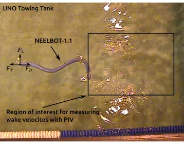
the field of anguilliform swimming, with the additional overlap amongst the PIV testing, eel-like robots, and hydrodynamic analysis. The red crosshair denotes the additional overlap which is the target contribution of this dissertation research. . . 15 1.4 Region of interest for measuring fluid flow velocities using PIV techniques. . . 16 2.1 Simplified schematic showing how the vortex distribution models the anguilliform

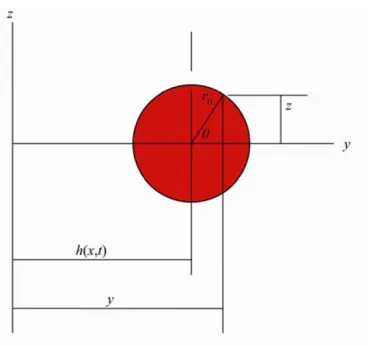
shape in a uniform flow for one instance in time. The centers of the 2-D vortices are constrained to the x-axis with the flow past vortex distribution (vortices are not to scale). The net circulation of this distribution is specified as 0 for all timet, while the magnitude and direction of the vortex distribution changes over time and space. The displacement distribution, h(x, t), is to be solved for based on these initial and boundary conditions. . . 19 2.2 Anguilliform element and wake geometry with associated variable naming. . . 24 2.3 Coordinates of the body cross-section. . . 27 2.4 Coordinate description of generalized oscillating strip, modeling the anguilliform

motion. . . 27 2.5 Annotations denoting the length parameters of the anguilliform shape for one time

step of the motion. . . 36 2.6 Theoretical anguilliform motion plotted for 10 equally spaced steps in time. . . 37 2.7 Computed velocity field vectors and velocity magnitude downstream of the ideal

robot shape motion for t = 0.0T. The superimposed shape function is what the doublets on they= 0 m centerline are modelling. . . 43 2.8 Computed velocity field vectors and velocity magnitude downstream of the ideal

(13)

2.10 Computed velocity field vectors and velocity magnitude downstream of the ideal robot shape motion for t = 0.3T. The superimposed shape function is what the doublets on they= 0 m centerline are modelling. . . 45 2.11 Computed velocity field vectors and velocity magnitude downstream of the ideal

robot shape motion for t = 1.0T. The superimposed shape function is what the doublets on they= 0 m centerline are modelling. . . 48 2.17 Schematic showing line integrals of circulation for the complete system and the

individual robot and wake systems, each of which is composed of discrete elements. 52 2.18 Computed velocity field vectors and velocity magnitude downstream of the actual

robot shape motion for t = 0.0T. The superimposed shape function is what the doublets on they= 0 m centerline are modelling. . . 52 2.19 Computed velocity field vectors and velocity magnitude downstream of the actual

(14)

2.26 Computed velocity field vectors and velocity magnitude downstream of the actual robot shape motion for t = 0.8T. The superimposed shape function is what the

doublets on they= 0 m centerline are modelling. . . 56

2.27 Computed velocity field vectors and velocity magnitude downstream of the actual robot shape motion for t = 0.9T. The superimposed shape function is what the doublets on they= 0 m centerline are modelling. . . 57

3.1 Free-body diagram of eel segmentn. . . 61

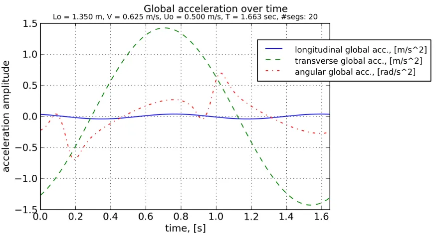
3.2 Global translational and angular accelerations of NEELBOT-1.1. . . 64

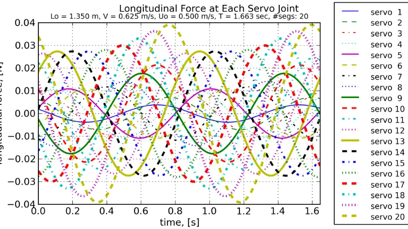
3.3 Longitudinal forces of NEELBOT-1.1 over time. . . 65

3.4 Longitudinal forces of NEELBOT-1.1 over time. . . 65

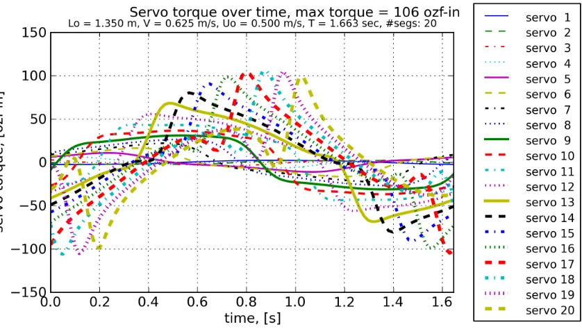
3.5 Servo torques of NEELBOT-1.1 over time. . . 66

3.6 Servo torques of the robotic eel over time with head fixed. . . 66

3.7 Rotational Speed-Torque curve for Dongbu Herkulex DRS-0201 (servo index 2). . . 67

3.8 NEELBOT-1.0 robot design (without waterproofing skin). (photo courtesy of UNO Marketing Dept.) . . . 68

3.9 Exploded view of two body segments and internal components (wiring omitted) of NEELBOT-1.0. . . 69

3.10 NEELBOT-1.0 swimming with waterproof skin. (photo courtesy of UNO Marketing Dept.) . 69 3.11 Rendering of NEELBOT-1.1 showing off its sleek curves. The green cylinders are the AAA batteries with 2 per segment, and the dark blue boxes are the servo-actuators. . . 71

3.12 Shown is the NEELBOT-1.1 without its waterproofing skin, but showing off its translucent body segment shells. The translucence allows the LED status lights of the servos to be visible during use. . . 72

3.13 Rendering of three segments and their joints of NEELBOT-1.1. The green cylinders are the AAA batteries with 2 per segment, and the dark blue boxes are the servo-actuators. The turquoise components in the head, which is the right-most segment, are the circuit boards used to communicate wirelessly with a desktop PC and transmit the servo commands down the length of the robot. Wiring is omitted, but it passes through the top of the segments inside very smooth passageways, minimizing friction. . . 74

3.14 LabVIEW code of the program that controls all motion aspects of NEELBOT-1.1. It reads in a shape function file, transmits the encoded data to a wireless transceiver, and receives and records the servo-actuator angles. . . 78

3.15 Buoyancy/mass distribution of NEELBOT-1.1. . . 81

3.16 Bottom side of NEELBOT-1.1 showing attached lead tape used as ballast. . . 82

3.17 Comparison of angles from different PIV testing “runs” versus time for servo 1. Despite the inaccuracy of the angles over time, the servo angle versus time for each test precisely agree with one another. . . 84

3.20 Coordinate system for 2 degree-of-freedom robot overlaid on multi-DOF robot. . . 90

3.21 PID independent joint control diagram. . . 94

(15)

3.23 Tracking error versus time for each joint, for a 2 degree of freedom system. . . 95

3.24 Spatial superposition of servo angles for all time steps for an advance speed of 0.0 m/s. . . 103

3.25 Spatial superposition of servo angles (blue) compared to the desired motion (black) for 10 evenly spaced time steps for an advance speed of 0.0 m/s. . . 103

4.1 PIV equipment installed on UNO Towing Tank carriage with rendering of NEELBOT-1.1 and its tether. . . 109

4.2 Components of the custom robotic eel tether and its coordinate system. . . 110

4.3 Components of the TSI Model 6800 SPIV System at University of New Orleans. . 111

4.4 Annotations showing the exact locations of the interested measurement region and the field of view of the PIV. . . 113

4.5 PIV field of view positions relative to the NEELBOT-1.1 frame of reference. . . 114

4.6 TSI Model 6800 SPIV system installed on UNO Towing Tank carriage, shown while underway during a test. NEELBOT-1.1 is the brightly illuminated object in the center of the picture. . . 115

4.7 NEELBOT-1.1 shown tethered in position in front of the PIV system. . . 116

4.8 Foil drag of robot vs. advance speed (Uo). . . 117

4.9 Straight-line drag of robot vs. advance speed (Uo). . . 118

4.10 Transverse Force. . . 123

4.11 For the advance speed of 0.0 m/s, the mean of transverse force for each time step is shown, with error bars showing standard deviation of the mean, i.e. the uncertainty.124 4.12 DFT of Transverse Force. . . 124

4.13 Filtered Transverse Force data. . . 125

4.14 Longitudinal Force. . . 125

4.15 For the advance speed of 0.0 m/s, the mean of longitudinal force for each time step is shown, with error bars showing standard deviation of the mean, i.e. the uncertainty. . . 126

4.16 DFT of Longitudinal Force. . . 126

4.17 Filtered Longitudinal Force data. . . 127

(16)

4.23 For the advance speed of 0.16 m/s, the mean of longitudinal force for each time step is shown, with error bars showing standard deviation of the mean, i.e. the

uncertainty. . . 131

4.42 Screenshot of recorded video of a motion programming test, that measured the angular positions of the joints over time. PIV testing is not being performed in this video, but the green laser would be shining in from the right, parallel to the plane of the image. . . 144

4.43 Schematic showing the iterative spirals occuring over the course of the research, with each spiral attempting to focus on all the aspects of the project related to determining the thrust/drag coefficients. . . 146

4.44 Sectional force coefficient distributions shown for every other timestep for the first half of the motion cycle of the ideal motion using the parameters from Table 2.1. This plot replicates the results graphed in Figure 8 of Vorus and Taravella (2011) except for different design parameters. . . 150

4.45 The sectional force coefficient is integrated over the length of the robot and then plotted over time for one cycle of motion clearly showing the two cycles of thrust production in that span. This is for the ideal motion case using the parameters listed in Table 2.1 . . . 151

(17)

4.47 The sectional force coefficient integrated over the length of the robot and then plotted over time for one cycle of motion clearly shows the two cycles of thrust production in that span. This is for the non-ideal motion case at a carriage advance speed of 0.0 m/s. . . 153 4.48 Sectional force coefficient distributions shown for every other timestep for the first

half of the motion cycle. This is for the non-ideal motion case at a carriage advance speed of 0.16 m/s. . . 153 4.49 The sectional force coefficient integrated over the length of the robot and then

plotted over time for one cycle of motion clearly shows the two cycles of thrust production in that span. This is for the non-ideal motion case at a carriage advance speed of 0.16 m/s. . . 154 4.50 Sectional force coefficient distributions shown for every other timestep for the first

plotted over time for one cycle of motion clearly shows the two cycles of thrust production in that span. This is for the non-ideal motion case at a carriage advance speed of 0.25 m/s. . . 155 4.52 Sectional force coefficient distributions shown for every other timestep for the first

plotted over time for one cycle of motion clearly shows the two cycles of thrust production in that span. This is for the non-ideal motion case at a carriage advance speed of 0.40 m/s. . . 156 4.54 Free-body diagram showing forces acting on tether and the robot. It is unknown

at this point in which direction the force is acting on the robot. . . 157 4.55 Free-body diagram showing the forces acting on the tether and robot, updated with

computed thrust prediction, Ff x, of the robot motion. From this, the drag force acting on the robot can be predicted. . . 157 4.56 Efficiency versus carriage advance speed for ideal and non-ideal motions. . . 159 4.57 NEELBOT-1.1 underway during a PIV test. . . 160 4.58 Screenshot showing example of seed particle density in the flow field (square grid

of 32 pixels; 32 pixels = 5.72mm. . . 161 4.59 Example of processed vectors showing good (green), bad (red), and interpolated

(yellow) vectors. Good vector percentage: Left frame: 95%; right frame: 91%. . . . 162 4.60 Several cycles of the velocity components shown for the specific spatial point of

x= 1301.3 mm, y=−143.86mm. . . 164 4.61 View of the fluid flow field showing the point in space where the time-series of data

in Figure 4.60 was recorded. . . 165 4.62 Data reordering technique to increase the sampling rate to an effective 80 Hz,

assuming the fluid flow is perfectly cyclic. . . 166 4.63 Reordered time series of velocity component data into one cycle to increase the

(18)

4.64 Magnitude of the Discrete Fourier Transform of the velocity component data in Figure?? . . . 169 4.65 Flow field of raw velocity vectors att= 0.0T forU0= 0.25 m/s. . . 170

4.66 Flow field of filtered velocity vectors at t= 0.0T forU0= 0.25 m/s. . . 171

4.67 Timesteps 0.0T, 0.1T, 0.2T, and 0.3T of filtered (fc= 3.625 Hz) velocities at equal

time steps over the robotic eel motion cycle forU0 = 0.25 m/s. The uniform flow

ofu= 0.25 m/s has been subtracted from the flow, giving the flow field an inertial frame of reference. . . 173 4.68 Timesteps 0.4T, 0.5T, 0.6T, and 0.7T of filtered (fc= 3.625 Hz) velocities at equal

ofu= 0.25 m/s has been subtracted from the flow, giving the flow field an inertial frame of reference. . . 174 4.69 Timesteps 0.8T and 0.9T of filtered (fc= 3.625 Hz) velocities at equal time steps

over the robotic eel motion cycle for U0 = 0.25 m/s. The uniform flow of u =

0.25 m/s has been subtracted from the flow, giving the flow field an inertial frame of reference. . . 175 4.70 Control volume of momentum integral analysis of anguilliform eel. . . 175 4.71 Component velocities of the flow field along a cross-section in they-direction,

com-paring theoretical and experimental values for timet= 0.0T. . . 178 4.72 Component velocities of the flow field along a cross-section in they-direction,

com-paring theoretical and experimental values for timet= 0.9T. . . 183 4.81 Comparison of momentum flux aty cross-section x= 1.15 versus time. The

com-parison is between the momentum flux calculated from the PIV and theoretical results. . . 184 4.82 Timesteps 0.0T, 0.1T, 0.2T, and 0.3T of filtered (fc= 3.625 Hz) velocities at equal

(19)

4.84 Timesteps 0.8T and 0.9T of filtered (fc= 3.625 Hz) velocities at equal time steps

0.16 m/s has been subtracted from the flow, giving the flow field an inertial frame of reference. . . 188 4.85 Timesteps 0.0T, 0.1T, 0.2T, and 0.3T of filtered (fc= 3.625 Hz) velocities at equal

time steps over the robotic eel motion cycle forU0= 0.0 m/s. . . 190

time steps over the robotic eel motion cycle forU0= 0.0 m/s. . . 191

4.87 Timesteps 0.8T, and 0.9T of filtered (fc= 3.625 Hz) velocities at equal time steps

over the robotic eel motion cycle forU0 = 0.0 m/s. . . 192

ofu= 0.40 m/s has been subtracted from the flow, giving the flow field an inertial frame of reference. . . 195 4.90 Timesteps 0.8T and 0.9T of filtered (fc= 3.625 Hz) velocities at equal time steps

0.40 m/s has been subtracted from the flow, giving the flow field an inertial frame of reference. . . 196 4.91 Trace of the approximate path of the disturbance due to the boundary layer

shed-ding for timestep 0.6T of the filtered (fc= 3.625 Hz) velocities for U0 = 0.25 m/s.

The uniform flow of u = 0.25 m/s has been subtracted from the flow, giving the flow field an inertial frame of reference. . . 196 4.92 Approximate locations of vortices that are assumed to be part of three-dimensional

vortex rings for timesteps 0.9T and 0.0T of the filtered (fc= 3.625 Hz) velocities

for U0 = 0.25 m/s. The uniform flow of u = 0.25 m/s has been subtracted from

the flow, giving the flow field an inertial frame of reference. . . 197 4.93 Time-sequence of 2nd distinct wake structure, a vortex pair being shed from the tail.198 5.1 Simplified schematic showing dynamics of unsteady foil in a free-stream fluid (the

lighter-colored outline contrasted with the darker-colored one denote the unsteady motion of the foil). . . 200 5.2 Schematic showing dynamics of the non-ideal design of the anguilliform robot

mo-tion (the lighter-colored outline contrasted with the darker-colored one denote the unsteady motion of the anguilliform shape). . . 200 5.3 Schematic showing dynamics of ideal design of the anguilliform robot motion (the

lighter-colored outline contrasted with the darker-colored one denote the unsteady motion of the anguilliform shape). . . 201 5.4 Illustration of shed boundary layer. . . 203 5.5 Proposed simplified model of the vortex shedding occurring for the non-ideal

(20)

LIST OF TABLES

Table

2.1 Current parameter values. . . 38

3.1 Dongbu Herkulex DRS-0201 physical characteristics and specifications. . . 77

3.2 Comparison of computed and actual masses and buoyancy. . . 83

3.3 Ziegler-Nichols tuning rules for the Second Method. . . 96

3.4 Heuristically/empirically determined values of Dongbu Herkulex DRS-0201 servo-actuator (insert columns showing measured and sys identification calculated values and maybe a range of values for confidence). . . 102

4.1 Table of advance speeds and tether positions of the robot. The value for each unique speed-tether position combination denotes the label number for the “run” performed during the experiment. A run consists of the carriage traversing the length of the tank during DAQ. . . 115

4.2 NEELBOT-1.1-tether system natural frequency analysis. . . 123

4.3 Percent difference between maximum amplitude of load cell measurements and theoretical predictions. . . 143

4.4 Details of iterative spirals. . . 145

(21)

ABSTRACT

An anguilliform swimming robot replicating an idealized motion is a complex marine vehicle necessitating both a theoretical and experimental analysis to completely understand its propulsion characteristics. The ideal anguilliform motion within is theorized to produce “wakeless” swimming (Vorus and Taravella (2011)), a reactive swimming technique that produces thrust by accelerations of the added mass in the vicinity of the body. The net circulation for the unsteady motion is theorized to be eliminated.

The robot was designed to replicate the desired, theoretical motion by applying control theory methods. Independent joint control was used due to hardware limitations.

The fluid velocity vectors in the propulsive wake downstream of the tethered, swimming robot were measured using Stereoscopic Particle Image Velocimetry (SPIV) equipment. Simultaneously, a load cell measured the thrust (or drag) forces of the robot via a hydrodynamic tether. The measured field velocities and thrust forces were compared to the theoretical predictions for each.

The desired, ideal motion was not replicated consistently during SPIV testing, producing off-design scenarios. The thrust-computing method for the ideal motion was applied to the actual, recorded motion and compared to the load cell results. The theoretical field velocities were com-puted differently by accounting for shed vortices due to a different shape than ideal. The theoretical thrust shows trends similar to the measured thrust over time. Similarly promising comparisons are found between the theoretical and measured flow-field velocities with respect to qualitative trends and velocity magnitudes. The initial thrust coefficient prediction was deemed insufficient, and a new one was determined from an iterative process.

(22)

distinct times during a half-cycle.

These qualitative and quantitative comparisons were used to confirm the possibility of the origi-nal hypothesis of “wakeless” swimming. While the ideal motion could not be tested consistently, the results of the off-design cases agree significantly with the adjusted theoretical computations. This shows that the boundary conditions derived from slender-body constraints and the assumptions of ideal flow theory are sufficient enough to predict the propulsion characteristics of an anguilliform robot undergoing this specific motion.

(23)

CHAPTER I

Introduction

(24)

to the inability to develop the robot with the proper actuators and rapid prototyping. In addition to the aspects stated above, this research is cutting into the relatively unknown field of underwater robotics, with the critical feature of needing to be waterproof. Most importantly, this robot can accomplish jobs that would otherwise place naval or scientific personnel at serious risk.

During the past few years of working on this research, one of the first questions I get asked is “what are the practical uses of a swimming anguilliform robot?” Unbelievably, there are an unlim-ited number of specific practical uses for an underwater robot imitating a biological anguilliform eel. More generally, there are three types of use considered at the moment. There is the ultimate use of it being a tool in the defense repertoire of the United States Navy in terms of searching for mines or adverse weapons in the littoral and riverine environments, which is explained in more detail in the next section. Secondly, this robot could be used by environmental scientists to monitor the world’s oceans, estuaries, and other bodies of water by carrying a suite of measurement tools such as salinometers, thermometers, raw video footage, etc., all while minimally affecting the natural surroundings. The third practical use is an academic one, of which this dissertation expounds on: the robot’s propulsive wake is being investigated in order to determine whether the theoretical hy-drodynamics compare to the experimentally measured results. More specifically, the theory consists of slender body theory describing the fluid flow about the robot and proper shifting, in time and in space, of hydrodynamic added mass to generate forward thrust, as opposed to typical first-order lift methods (see Vorus and Taravella (2011) for more details). The experimentally measured results are obtained by cameras imaging the downstream flow which is illuminated and recorded by lasers reflecting off neutrally-buoyant seed particles. Successive images are cross-correlated in order to compute velocity vectors over the entire flow field for each instance in time. Practically, the prov-ing (or disprovprov-ing) of this theory will provide for a better design of a swimmprov-ing anguilliform robot for the next prototype. This dissertation elucidates the theory involved in specifying the swim-ming motion, the development of the swimswim-ming prototypes, the experimental measurements of the wake field’s velocities, and finally the conclusions found from the comparison of the theoretical and experimental results.

(25)

how this project contributes to that part of the field. Chapter 2 provides an explanation of the two- and three-dimensional derivations of this highly efficient anguilliform swimming motion using the assumptions of ideal flow theory applied to slender bodies. Extensions are made to the original derivation in order to apply the theory to a non-ideal shape, or off-design recorded motion of the actual robot. Chapter 3 illustrates the design-build development of the prototypes by explaining the physics-based model used to predict joint loads and also the product development of the actual robots, which included in-house fabrication. Precise development was critical to ensure the robot can attain the desired motion. Chapter 4 details the experimental testing required to measure the wake velocities using Particle Image Velocimetry (PIV) equipment and the propulsive forces generated by the swimming motion. Supporting factors such as the experimental hardware setup and the post-processing software that analyzes the recorded data to compute the velocity vectors are explained. Chapter 5 states the conclusions determined from all the facts gathered throughout the entire research process. These conclusions tie in all aspects of the theory and the experiment and provide a comparison to the overall field of associated research. A call to future work and improvements and additions beyond the current research is made.

1.1 Mission Objectives and Motivation

The primary objective of the research explained within is to contribute academically to the field by comparing experimental results to that of an improved development of the swimming motion. A secondary objective that is beyond the scope of this dissertation’s objectives is that this research will aid in producing a functional, practical prototype that can be further developed and refined for use in a Naval Intelligence, Surveillance, and Reconnaissance (ISR) mission, an inspection or search-and-rescue (SAR) mission, or aid in scientific research of the world’s oceans by measuring and monitoring key variables such as acidity, salinity, and temperature.

(26)

con-Underwater Vehicles (AUVs), with low acoustic, radar, and optical signatures, to carry sensors into dangerous areas, like harbors and streams, in support of ISR missions. This project contributes to the investigation of the science and engineering aspects of a new type of AUV that could eventually meet some special Naval maritime sensing and stealth objectives. It is believed that a small, nearly undetectable vehicle capable of autonomous, long-range sub-surface missions would be capable of accomplishing these tasks.

The types of sensors that can be placed on the head of the robot are only limited by their size and power requirements allowed by the robot. The robot can be used for search-and-rescue missions to scan the seafloor using SONAR (Sound Navigation and Ranging) for sunken vessels or missing airplanes such as the recently lost Malaysian Airline Flight MH370 (Wikipedia (2015b)). With an ultrasonic sensor or even video camera for immediate human-readable feedback, this robot could also be used to inspect the hundreds of miles of undersea oil and gas pipelines over the world, which are a threat to the wildlife if unchecked as shown by the recent pipeline failure off the coast of California (Wikipedia (2015a)). With its bio-mimicry, the robot would be minimally invasive to the surrounding environment during any of its missions. From a scientific research standpoint, the robot could contain a suite of sensors related to monitoring the world’s oceans, especially considering the need to measure variables that may be harbingers of climate change, such as ocean acidity or temperature.

Most unbelievably, this robot could theoretically propel itself for unlimited periods of time, in addition to it already predicted to be highly efficient due to no induced vortices being shed. Once its batteries begin to run low, it could attach itself to the seafloor, vertical pile, or catenary chain and then let the ambient ocean currents run past it inducing an oscillating motion along the length of the robot, forcing the actuators to act as generators and recharge its batteries. The only limits would be its ability to attach to an object in time and the number of times the batteries can be recharged.

It is amazing to think that the idea for this possible AUV stems from a fishing trip by Dr. Vorus, on which he noticed a “water snake slithering through the surfactant field of spring pollen covering the surface of a farm pond.” According to him, “the animal left a very clean and distinct serpentine track of its progression through the pollen, barely wider than the width of its body.”

(27)

occur with a careful specification of the deformation mode shape (Saffman (1967) and Miloh and Galper (1993)). With the fluid assumed ideal, vortex shedding, rotational wake, and induced drag would not occur. The implication is that for a real fluid, provided the existence of a thin boundary layer, similarly configured bodies with the same deformation mode shape self-propel without vortex shedding, rotational wake, and induced drag (Vorus (2005)). Only viscous drag effects, due to the existence of the thin boundary layer, are present and unavoidable. The motion mode examined by Vorus (2005) is the little-exploited anguilliform mode exhibited in some aquatic animal swimming; the Anguilla includes the snake, eel, lamprey, and leach, among others. The anguilliform swimming differs from the high-speed carangiform and tunniform fish swimming in that the thrust is produced by more global body motions, rather than by the flapping of the lunate tail of the latter high-speed group.

Researchers have been studying the anguilliform swimming motion for quite some time. Some notable works include that of Wu (1961) and Lighthill (1970), with the “elongated body theory” in the Appendix of Lighthill (1960) being the basis for several recent analyses. Besides the recent works of Vorus (2005) and Vorus and Taravella (2011) directly related to this project, there have been other recent works expanding on the theoretical hydrodynamic analysis of the anguilliform motion such as Carling et al. (1998), Pedley and Hill (1999), and Cheng and Chahine (2001). Key points and results of these analyses are described in more detail in the Literature Survey section to follow.

(28)

Figure 1.1:

Venn diagram showing the different areas of concentration within or related to the field of anguilliform swimming.

Figure 1.2:

(29)

1.2 Literature Survey

Going back close to a century, several similar and dissimilar studies have preceded this one, shedding light on both carangiform and anguilliform swimming motions ranging from ideal flow theories to PIV testing of live lamprey and anguilla eels to novel numerical techniques that solve the Navier-Stokes equations as applied to these motions. (Carangiform motions will be mentioned briefly throughout the text for comparison, but anguilliform swimming is the sole focus.)

The modern names of anguilliform and carangiform date back to Breder, 1926 (cited in Tytell and Lauder (2004)), but the kinematic distinction between the two have been known for years before that (Marey, 1895 and Alexander, 1983 (cited in Tytell and Lauder (2004)). Distinguishing the kinematic differences between the two was relatively easy; understanding the hydrodynamics of either has been much less understood but studied thoroughly. Some of the first to propose theories on how anguilliform swimming motions can produce thrust include Gray (1933a), Gray (1933b), Taylor (1952), and Lighthill (1960).

With several photographs of eels over a short period of time, Gray (Gray (1933a) and Gray (1933b)) was the first to quantitatively study the body movement of eels and their propulsive mechanism by showing that the body undulations have the form of a backward traveling wave. He determined the now obvious intuition that the longitudinal component of the pressure normal to the eel body is equal to its resistance. Among other things, he determined that the magnitude of the thrust is based on the velocity of the transverse movement of the body and the angle that the mean path of motion makes with the surface of the body while it crosses this line over time. While observing swimming dolphins, Gray is most known for the formulation of his paradox which states that a dolphin swimming at 20 knots cannot have enough muscle to propel itself forward at that speed (Gray (1936)). This paradox has prompted several succeeding researchers to take up the cause and investigate the thrusts of swimming animals, particularly anguilliform eels.

(30)

heat conduction equation as an analog for the tangential stresses, Taylor computes the longitudinal component of force on the cylinder. He then computes the power done on the fluid by the eel for varying parameters to compute the speed at which the eel propels itself at the least energy output.

I am skipping several decades for now and focusing on the last 20 years where more PIV analysis

has been done on swimming eels and other fishes; also force estimates from wake measurements.

In the last two decades, several studies have been performed on the wake measurements of swimming fishes (or similarly dynamic, flying animals) using PIV or numerical CFD techniques (Anderson (1996); Müller et al. (1997); Müller et al. (2001); Drucker and Lauder (1999); Nauen and Lauder (2002); Nauen and Lauder, 2002b; Tytell and Lauder (2004); Tytell (2004), (previous articles all cited by Tytell (2004); Borazjani and Sotiropoulos (2009); to name a few). An even fewer number have focused on anguilliform motions: Müller et al. (2001), Borazjani and Sotiropoulos (2009), Kern and Koumoutsakos (2006), Tytell and Lauder (2004), Tytell (2004), Hultmark et al. (2007), Leftwich and Smits (2011), Pedley and Hill (1999), Carling et al. (1998)

Carling et al. (1998) does not predict complex vortical structures and lateral jets. They used a 2-D CFD model to estimate the flow fields behind a self-propelled anguilliform swimmer. Their calculations indicated a single, large vortex ring wrapping around the eel, with the eel in the center, producing upstream flow behind the eel, which has not been verified by any experimental measurements on live eels.

Pedley and Hill (1999) state that the load against which the swimming muscles contract, during the undulatory swmming of a fish, is composed principally of hydrodynamic pressure forces and body inertia. In the past, this has been analyzed through an equation for bending moments for small-amplitude swimming, using Lighthill’s elongated-body theory and a vortex-ring panel method to compute the hydrodynamic forces (). They do find that the wake morphology resembles that of a reverse von Karman vortex street, which is not the 2P wake structure found by the majority of other authors.

M¨uller et al. (2001) found that the anguilliform wake structure is 2P and was the first to experimentally measure the wake structure of eels using PIV techniques.

(31)

They investigate the interaction between body movements and the flow around swimming eels using 2-D PIV. The wake behind eels swimming at 1.5 L/s consisted of a double row of vortices with little backward momentum (NEELBOT-1.1 swims at 0.185 L/s for the nominal design speed, for comparison). The eel sheds two vortices per half tail-beat, which can be identified by their shedding dynamics as a start-stop vortex of the tail and a vortex shed when the body-generated flows reach the ’trailing edge’ and cause separation. Two consecutively shed ipsilateral body and tail vortices combine to form a vortex pair that moves away from the mean path of motion. This wake shape resembles flow patterns described previously for a propulsive mode in which neither swimming efficiency nor thrust is maximized but sideways forces are high. The described wake shape is illustrated in B of Fig ??. It has since been found by later researchers that most of the thrust occurs near the end of the tail, correcting these findings that the entire body produces some form of thrust.

(32)

idea that the thrust and drag cancel out for steady-state swimming, producing a control volume of zero momentum. They attribute the increase to the movement of the eel’s snout. They go on to state that while thrust cannot be measured directly from the wake of swimming eels, it is still useful, conceptually to separate it from drag. By using a mathematical model, such as EBT or more complex CFD models (Carling et al. (1998); Wolfgang et al. (1999); Zhu et al., 2002), thrust can be estimated and used to calculate a Froude propulsive efficiency. They estimate the efficiency using their measured wake power to be between 0.43 and 0.54. Using EBT, they estimate the efficiency to be 0.87.

As a follow-up to his previous paper, Tytell and Lauder (2004) again investigates the hydrody-namics of eel swimming using PIV but this time applied to the effect of swimming speed. After investigating American eels, Anguilla rostrata, at swimming speeds ranging from 0.5 to 2.0 Ls−1

(33)

quasi-steady drag forces normal and tangential to the body midline using the kinematics, in a similar way to Jordan, 1992. The normal and tangential drag coefficients were estimated according to empirical descriptions of turbulent flow normal to a cylinder (Taylor (1952); Hoerner, 1965) and parallel to a flat plate (Hoerner, 1965). Wake power was not calculated from the resistive model because it does not explicitly account for how power is shed into the wake. Vortex ring impulse and force were estimated (compare his method here to that of others such as Spedding et al. (1984) and Dabiri (2005)?). Impulse generated at the tail tip was also estimated from the first moment of vorticity (Birch and Dickinson, 2003), averaged over half a tail beat, with the force being estimated by taking the time derivative. The power required to produce the wake was determined by inte-grating the kinetic energy flux through a CV strip downstream of the eel. Additionally, a lateral power was estimated by assuming the small and relatively noisy axial component of velocity was zero and integrating only the lateral velocity contribution to the kinetic energy flux. The cost of producing the wake was estimated by dividing the wake power by the swimming speed. This cost is one component of the total mechanical cost of transport, which also includes the thrust power and the inertial power required to undulate the body. Tytell (2004) found the Strouhal number to stay approximately constant at 0.324±0.003, and that the amplitude grows slightly with higher swimming speed (as contrasted with Borazjani and Sotiropoulos (2009) and Vorus and Taravella (2011)). However, he does state that tail tip velocity seems to be the kinematic parameter that most affects the flow in the wake. He did find that eels maintain a constant Strouhal number within a single swimming speed by varying tail beat frequency inversely with amplitude. While Froude propulsive efficiency would be useful to estimate, it requires a measurement of thrust, which cannot be estimated due to the lack of axial flow in the wake. However, changes in the cost of producing the wake, one component of the total cost of transport, may indicate trends in propulsive efficiency. At all speeds except the highest, an eel’s tail functions like a vortex ring generator (Shariff and Leonard, 1992), adding circulation to the fluid at a rate proportional to its velocity squared.

(34)

plitude towards the tail. Most of the thrust production was found to occur at the tail, countering M¨uller et al. (2001)’s findings. The wake was found to consist of a double row of vortex rings with an axis aligned with the swimming direction and that these vortex rings were responsible for producing lateral jets of fluid, which has also been documented in Tytell and Lauder (2004) and Tytell (2004).

(35)

Similar to the 2P wakes found in Hultmark et al. (2007), Tytell and Lauder (2004), and M¨uller et al. (2001), Borazjani and Sotiropoulos (2009) used a customized numerical scheme to compute the hydrodynamics of anguilliform swimming in the transitional and inertial flow regimes. They call their CFD method an “immersed boundary method” and vary the St and Re numbers, but kinematically, their motion is slightly different than that of the NEELBOT-1.1’s in that they allow the head to move laterally. They found that the net mean force to be mainly dependent on the tail-beat frequency rather than the tail-tail-beat amplitude, which is also the case for the theory developed by Vorus and Taravella (2011) in that the higher speeds require a smaller tail amplitude. The critical Strouhal number, St∗, at which the net mean force becomes zero is a decreasing function of Re and approaches the range of St numbers at which most anguilliform swimmers swim in nature (St= 0.45 according to these authors, contrasted withSt= 0.3−0.35 according to others such as Leftwich and Smits (2011), Hultmark et al. (2007), Tytell and Lauder (2004)). They find that the propulsive efficiency of anguilliform swimmers at St∗ is not an increasing function of Re

but instead is maximized in the transitional turbulence regime. They show that the form drag decreases while viscous drag increases as St increases. Their simulations reinforce their previous studies (Borazjani and Sotiropoulos (2008)) that the 3-D wake structure depends primarily on the Strouhal number. They separate the hydrodynamic thrust and drag contributions according to a force decomposition approach proposed by Borazjani and Sotiropoulos (2008). For all simulated

(36)

The authors show illustrations of four wake cases for varying Re and St numbers, pointing out that three are drag-type and the fourth is thrust-like. For two of the drag-type cases, the net flux of the 3-D wake rebuts the original claim and proves that they are in fact thrust-type. Along with the claim by Dabiri (2005), this underscores the difficulty in assessing the wake type from velocity measurements at 2-D planes. Their results confirm that for a fixed Reynolds number, both single- and double-row wake structures can emerge depending on the St number, which is to be expected since the Strouhal number can be viewed as the ratio of the mean lateral tail velocity to the axial swimming velocity. The authors visualize the 3-D structure of anguilliform wakes by plotting instantaneous iso-surfaces of the q-criterion (Hunt et al., 1988). For low St, a single row pattern emerges while at higher St, the double-row structure is observed. For the Re = 4000 case, the structure observed is very similar to that obtained in the pitching panel experiments by Buchholz and Smits (2006).

(37)

Figure 1.3:

Venn diagram showing the different areas of concentration within or related to the field of anguilliform swimming, with the additional overlap amongst the PIV testing, eel-like robots, and hydrodynamic analysis. The red crosshair denotes the additional overlap which is the target contribution of this dissertation research.

may be attributed to separation as noted by Sarpkaya (). The authors compute the instantaneous momentum flux in the streamwise direction over an entire cycle using the integral form of the momentum equation . The authors find that there is a 27% difference in their mean thrust compared to the slender body theory of Lighthill (1960), noting that their method is only 2-D and that of Lighthill is 3-D. The authors concluded that pressure increased rapidly closer to the tail, indicating thrust production occurs closer to the tail. They show that the pressure signal correlates to the fluid structures passing the port, indicating that the organization of the vorticity in the boundary layer is directly linked to the unsteady thrust force produced by an anguilliform swimmer.

1.3 Current Research and Contributions to the Field

(38)

Figure 1.4: Region of interest for measuring fluid flow velocities using PIV techniques.

by combining the PIV testing of an anguilliform robot and a classical hydrodynamic analysis to compare and contrast the experimental and theoretical results. With that being said, the work of Hultmark et al. (2007) and Leftwich and Smits (2011) is very similar in that it investigates a robot with downstream PIV measurements, but it does not contribute a theoretical hydrodynamic analysis to support or disprove their measurements.

This research encompasses developing and building an anguilliform swimming robot to replicate the desired motion predicted by a classical hydrodynamic analysis. Particle Image Velocimetry (PIV) equipment then measured the wake field velocities produced by the robot, and these re-sults were compared to the predicted hydrodynamics. Figure 1.4 shows the final robot prototype, NEELBOT-1.1, swimming on the free surface of the Towing Tank of UNO (University of New Orleans) and a schematic showing the interested wake region behind it. Several assumptions are taken with both the theory and the experiment, but the evidence is still conclusive enough to draw comparisons between the two. Simply, slender-body theory is a very good tool used to predict the propulsion and hydrodynamics of this type of marine vehicle.

(39)

thrust by first-order lifting processes. The motion explained within is theorized to produce thrust via the reactive forces of accelerated added mass along the length of the robot. This process results in zero induced drag and zero shedding of vortices. The testing results presented within show that this type of propulsion is still possible, despite very few previous research affirming the same.

(40)

CHAPTER II

Theoretical Development

This chapter provides an explanation of the two- (Section 2.1.1) and three-dimensional (Section 2.1.2) derivations of the highly efficient anguilliform swimming motion using the assumptions of ideal flow theory applied to slender bodies, which produce the so-called ideal anguilliform swimming theory. Extensions are made to the original 3-D derivation in order to apply the theory to a non-ideal shape, or rather, an off-design recorded motion of the actual robot (Section 2.2.2).

2.1 Ideal Anguilliform Swimming Theory

The dominant feature of the ideal swimming theory is the constraint that the circulation is continuously zero about the shape for all time, which produces the resulting condition of no shed vortices and no induced drag — “wakeless swimming.” The 2-D and 3-D formulations differ in how the physical shape of the anguilliform eel is modeled in the flow. The 2-D one is represented by vortices, whereas the 3-D uses doublets. The singularities for each case are constrained to the

x-axis.

2.1.1 2-D Formulation

(41)

Figure 2.1:

Simplified schematic showing how the vortex distribution models the anguilliform shape in a uniform flow for one instance in time. The centers of the 2-D vortices are con-strained to thex-axis with the flow past vortex distribution (vortices are not to scale). The net circulation of this distribution is specified as 0 for all timet, while the magnitude and direction of the vortex distribution changes over time and space. The displacement distribution,h(x, t), is to be solved for based on these initial and boundary conditions.

The general oscillatory displacement form of the anguilliform motion is specified as

h(x, t) =<{H(x)e−iωt} (2.1)

where h(x, t) is the transverse displacement of the shape function as shown in Figure 2.4. A particular and non-trivial solution to this equation is shown to be derived in Vorus (2005), and a brief overview is given here.

After deriving a trivial motion that produces no fluid disturbance at all, Vorus (2005) specifies the velocity term on the right-hand side of the linearized slender-body theory equation as the Biot-Savart law in terms of an axis vortex distribution:

ht(x, t) +Uohx(x, t) = 1 2π

Z L

0

γ(ξ, t)

x−ξ dξ (2.2)

(42)

An additional condition is required on γ(ξ, t) in that “wakeless” motion requires that the time rate-of-change of element circulation remain continuously zero. That is, the net circulation of the element, as represented by the integral of γ over the element length, must be zero at all time. This necessary constraint is accomplished withγ specified as periodic in both space and time, with body length L now being some multiple m of the fundamental spatial wave length of the vortex distribution, L/m. Figure 2.1 shows a simplified schematic of the vortex distribution along the

x-axis modeling the unknown anguilliform shape, h(x, t), in a uniform flow.

The vortex distribution is specified as a traveling wave of length L and frequency ω; the wave length of h(x, t) is defined as λ, which is equal to L only for the trivial case. The form of the prescribed vortex distribution is therefore:

γ(x, t) = Γ(x) cos

2πx L −ωt

=<hΓ(x)ei(2πxL −ωt)

i

(2.3)

The amplitude Γ(x) is taken as real but, at this point, as unspecified.

The following non-dimensionalization’s are used by using the nominal length, L, and wave displacement speed,V (ro is the radius of the circular cross section):

ro =

ro

L h(x, t) =

h(x, t)

L x= x

L t=

V t L

Substituting in the non-dimensionalization’s but dropping the overbars for clarity, the equation above becomes

γ(x, t) =<nΓ(x)e2πi(x−t)

o

(2.4)

In addition to satisfying the condition that the integral of γ(x, t) over the length L be identically zero at all t, the vortex distribution must satisfy the “shockless entry” condition γ(0, t) = 0 at the leading edge, as well as the “Kutta” condition γ(1, t) = 0 at the trailing edge. These three conditions are all appropriately satisfied by interpreting Γ(x) as the generalized function:

(43)

where the Heaviside step function,He(X), is defined as (Lighthill (1964)):

He(X) =

      

0 if X <0

1 if X ≥0

(2.6)

Multiplication of this generalized function with the traveling wave exponential in equation 2.4 achieves the continuously zero-lift requirement. This box idealization is a valid theoretical approxi-mation of the edge conditions at this level of analysis, asγ(x, t) by 2.4 is involved only in integration at 2.2, and never in differentiation.

Substitution of 2.4 into 2.2 gives the following first-order linear differential equation for H(x):

Hx(x)− 2πi

U Ht(x) =

Γ

UΛ(x) (2.7)

with

Λ(x)≡ 1 2π

Z 1

0

e2πiξ

x−ξdξ (2.8)

The solution of this differential equation is

H(x) =e2πixU

H(0) + Γ

U

Z x

0

e−2UπiξΛ(ξ)dξ

(2.9)

The term H(0) is the leading-edge displacement amplitude. The product of the leading factor and the H(0) term in the brackets represent a sinusoidal wave in x, the amplitude of which is modified over the length of the element, 0 ≤ x ≤ 1, by the second term. The dimensional wave length,λ, of the function is established by the leading factor in 2.9. This dimensional wave length is

λ=LUo

V (2.10)

and the time period, T =L/V, creates the following equation

T = L

V = λ Uo

(44)

at strip speed Uo is the same as the time required for the wave to advance one strip length L at wave speedV.” Reorganizing, it becomes

λ L =

Uo

V (2.12)

and this states that “the wavelength ratio is equal to the advance ratio for wakeless swimming to occur.” When both sides of this equality are unity, this becomes the trivial case. For other cases when this equality is true, this is the kinematic condition where non-zero axial load is developed but with necessarily unity ideal efficiency because vortex shedding does not occur.

Returning to the displacement amplitude distribution of equation 2.9, H(0) and Γ are the un-known parameters to be found, assuming the advance ratioU is specified. The head amplitude can be eliminated in terms of the total mean thrust coefficient, CT. Prior to this, a force consideration of the articulating anguilliform shape can be performed via a momentum integral analysis to obtain the thrust coefficient:

CT(t) = 2(1−U)

Z 1

0

γ(x, t)hx(x, t)dx (2.13)

Substitute equations 2.1 and 2.4 to obtain

CT(t) = Γ(1−U)<

Z 1

0

Hx(x)e−2πixdx+e−4πit

Z 1

0

Hx(x)e2πixdx

(2.14)

Using the derivation by Vorus (2005) ofCP(t) =U CT(t) in the above, the head amplitude can be eliminated in terms of the total mean thrust coefficient:

CT =

CP

U = 2π

Γ

U(1−U)<

i

Z 1

0

H(x)e−2πixdx

(2.15)

With another definition of CP:

CP(t) =