RESEARCH
Implications of construction method
and spatial scale on measures of the built
environment
Julie Strominger
1, Rebecca Anthopolos
2and Marie Lynn Miranda
2,3,4,5,6*Abstract
Background: Research surrounding the built environment (BE) and health has resulted in inconsistent findings. Experts have identified the need to examine methodological choices, such as development and testing of BE indices at varying spatial scales. We sought to examine the impact of construction method and spatial scale on seven meas-ures of the BE using data collected at two time points.
Methods: The Children’s Environmental Health Initiative conducted parcel-level assessments of 57 BE variables in Durham, NC (parcel N = 30,319). Based on a priori defined variable groupings, we constructed seven mutually exclu-sive BE domains (housing damage, property disorder, territoriality, vacancy, public nuisances, crime, and tenancy). Domain-based indices were developed according to four different index construction methods that differentially account for number of parcels and parcel area. Indices were constructed at the census block level and two alternative spatial scales that better depict the larger neighborhood context experienced by local residents: the primary adja-cency community and secondary adjaadja-cency community. Spearman’s rank correlation was used to assess if indices and relationships among indices were preserved across methods.
Results: Territoriality, public nuisances, and tenancy were weakly to moderately preserved across methods at the block level while all other indices were well preserved. Except for the relationships between public nuisances and crime or tenancy, and crime and housing damage or territoriality, relationships among indices were poorly preserved across methods. The number of indices affected by construction method increased as spatial scale increased, while the impact of construction method on relationships among indices varied according to spatial scale.
Conclusions: We found that the impact of construction method on BE measures was index and spatial scale specific. Operationalizing and developing BE measures using alternative methods at varying spatial scales before connecting to health outcomes allows researchers to better understand how methodological decisions may affect associations between health outcomes and BE measures. To ensure that associations between the BE and health outcomes are not artifacts of methodological decisions, researchers would be well-advised to conduct sensitivity analysis using different construction methods. This approach may lead to more robust results regarding the BE and health outcomes.
Keywords: Built environment, Neighborhood measures, Construction method, Spatial scale
© 2016 Strominger et al. This article is distributed under the terms of the Creative Commons Attribution 4.0 International License (http://creativecommons.org/licenses/by/4.0/), which permits unrestricted use, distribution, and reproduction in any medium, provided you give appropriate credit to the original author(s) and the source, provide a link to the Creative Commons license, and indicate if changes were made. The Creative Commons Public Domain Dedication waiver (http://creativecommons.org/ publicdomain/zero/1.0/) applies to the data made available in this article, unless otherwise stated.
Background
The built environment (BE) is defined as the “human-made space in which people live, work, and recreate on a day-to-day basis” and includes the physical condition of
homes, outdoor spaces, roads, sidewalks, and schools [1]. Previous research has found poor quality BE, measured by domains such as housing quality and nuisances, to be adversely associated with a multitude of human health outcomes, such as preterm birth [2], mental health [3–7], and childhood weight status [8, 9]. Despite evidence of a deleterious relationship between BE and health, findings remain inconsistent, with several studies showing null
Open Access
*Correspondence: [email protected]
3 Department of Statistics, Rice University, 6100 Main Street, MS-2,
Houston, TX 77005, USA
associations [10–13]. Such results have led researchers to hypothesize that inconsistent findings may be an arti-fact of methodological choices, thus prompting a call for an examination of methodology in the development of measures of the BE [12, 14–16].
Existing studies have documented the varying ways of first measuring and then operationalizing BE measure-ment in health outcomes research. In constructing BE measures of the physical neighborhood environment, source data have been derived from perceived and observed data [17], with subsequent metrics developed using geographic information system (GIS) methods and data reduction techniques [12, 14, 17]. Addition-ally, spatial scale has been identified as a source of vari-ation among BE measures [12, 15], with BE measures largely operationalized based on administratively-defined geographic units like census tracts or tax parcels [18]. Alternatively, researchers may construct neighborhoods based on community-defined neighborhood boundaries [19]. Thus, in health outcomes research, the potential for methodological choice to substantively impact study findings is widely understood [12, 14, 20, 21], and in light of methodological heterogeneity, the difficulty in making inter-study comparisons is not surprising [15].
To date, while researchers frequently examine the impact of certain methodological choices in construct-ing BE measures on a given association of scientific interest, for example, by estimating associations at alternative buffer sizes or census geographic units [18,
22, 23], to our knowledge, few studies have focused on the consequences of these choices on BE measure-ment itself [22, 24–26]. The few studies that have inves-tigated the impact on BE measurement are focused on measuring the food environment and green space [25,
27]. Absent from the literature is a systematic assess-ment of methodological choices in the construction of BE measures related to different BE domains. In this study, we respond to researchers’ calls for a methodo-logical assessment of BE measures in terms of stand-ardization related to underlying geography and spatial scale of measurement [12, 15, 16]. Using objective sur-vey data from a BE assessment tool conducted in Dur-ham, NC during 2008 and again in 2011, combined with supplemental administrative data on renter occupancy tenure and crime, we develop seven BE indices (hous-ing damage, property disorder, territoriality, vacancy, public nuisances, crime, and tenancy) according to four different index construction methods that alternatively account for number of parcels and parcel area. We apply three spatial scales that differentially account for the spatial structure of the study area. We investigate the implications of construction method and spatial scale on BE measures.
Methods
Study area
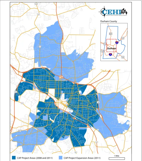
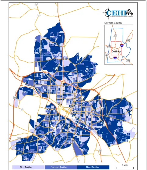
Figure 1 presents the study area that encompasses the urban core of Durham, North Carolina. In 2008, the study area comprised 886 census blocks (N = 17,225 parcels); in 2011, the study area was enlarged to include additional contiguous census blocks (total N = 1380 cen-sus blocks, 31,839 parcels).
Objective tax‑parcel survey data
The design and data collection for the Community Assessment Project (CAP) has been described in detail elsewhere [28]. An objective tax-parcel level survey, the CAP was built using a GIS data systems architecture. Equipped with handheld global positioning systems units, teams of trained raters collected data from the sidewalk or street. Fifty-seven variables, determined based on lit-erature review and feedback from the Durham commu-nity, were recorded [29–31]. Variables related to land use; occupancy status; the presence of nuisances such as litter and graffiti; evidence of territoriality such as barbed wire and fencing; and the physical condition of any buildings, yard, or property, were documented. Residential, com-mercial, and other property types were similarly assessed. Excluding land use and occupancy status, variables were assessed for presence or absence for each parcel in the study area. Land use was recorded as commercial, com-munity, empty lot, faith, government, parking lot, prop-erty, or residential type. For occupancy status, each parcel was recorded as either unoccupied or occupied.
The inter-rater reliability (IRR) of the CAP data was calculated across seven raters for each of the variables using 2011 data. The average agreement over the vari-ables was 0.95 (95 % CI 0.945, 0.953), well-above the con-ventional threshold of 0.70 for strong agreement [32]. While IRR was not computed for 2008, the same supervi-sor administered the training, and materials and modules were consistent between time periods, which would sug-gest a similarly strong IRR in 2008.
Supplementary data
Variable groupings
We grouped the CAP survey variables into five distinct domains: housing damage (e.g., boarded doors and roof damage), property disorder (e.g., litter and broken glass),
territoriality (e.g., fencing and security signs), vacancy, and public nuisances (e.g., graffiti and cigarette butts) (Addi-tional file 1: Table S1). Nuisances that were on or within 2 feet of public space were recorded as public nuisances,
while nuisances that were on private property beyond 2 feet from public space were recorded as property disorder.
Spatial scale
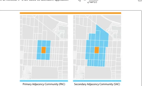
We constructed the seven BE indices at the census block level and two alternative spatial scales defined by adja-cency. The first, primary adjacency community (PAC), refers to the index block along with adjacent blocks that share a boundary, in the form of a vertex or line segment. The PAC is specified by constructing a first order adja-cency matrix. Explicitly, let W be a symmetric matrix with dimensions equal to the total number of blocks in the study area. If census blocks j and i share a vertex or line segment, then entry wij = 1; otherwise, wij = 0. Since in our analytical context, we consider a block to be a neighbor to itself, we set the diagonal entries wii = 1. The secondary adjacency community (SAC) extends the PAC by additionally including secondary neighbors (see Fig. 2) in the adjacency matrix construction. The mean geographic area among census blocks was 0.05 square kilometers (SD = 0.10). For PAC and SAC, the mean geo-graphic area was 0.52 (SD = 0.55) and 1.56 (SD = 13.39) square kilometers, respectively.
Alternative index constructions
The four index construction methods, hereafter referred to as Methods 1–4, are based on alternative approaches
to standardizing the variables (e.g., litter of the public nui-sances index) composing each BE index. Methods 1–4 are replicated for each of the three spatial scales. For a given method and spatial scale, standardized variables repre-senting each domain are summed together, yielding a BE domain-specific score (e.g., standardized litter + stand-ardized graffiti + standardized garbage, etc. = property disorder measure). Below, we explicate the development of Methods 1–4 using Method 1 as the heuristic example.
Method 1 aggregates each variable to a given spatial scale, resulting in a count (e.g., count of parcels with litter present in a census block). This count is then standard-ized to have mean 0 and standard deviation (SD) 1. Let cbp be an indicator for the presence of variable c in the pth parcel in spatial unit b. Then, for the p=1,. . .,Pb
parcels in spatial unit b, the count of a given variable pre-sent for all parcels in the index spatial unit is defined as
We then standardize this count by subtracting the aver-age count over the spatial units in the study region and dividing by the SD in the study region. Explicitly, the standardized count for a given variable is
(1) cb=
Pb
p=1
cbp.
(2)
cStdb = √cb− ¯c
var(c),
such that cStd
b ∼N(0, 1).
Within each BE domain, the standardized counts of variables are summed to yield an index value for each spatial unit. Formally, for a given BE domain BE in spatial unit b, we have
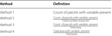
Method 2 extends Method 1 by dividing the count by the number of parcels in a given spatial unit, resulting in an average count per parcel (e.g., average count of litter per parcel in a census block). Instead of number of par-cels, Method 3 analogously accounts for geographic area, resulting in an average count per unit area (e.g., average count of litter per unit area in a census block). Method 4 uses an alternative approach to account for the underly-ing area by aggregatunderly-ing the area with a variable present over the spatial unit and then dividing by the total area, resulting in the proportion of area in a spatial unit with a variable present (e.g., the proportion of the total area in a census block with litter present). As in Method 1, vari-ables composing a given BE measure are summed to yield a BE domain-specific score. Table 1 summarizes the dif-ferent construction methods.
Statistical analyses
For all BE indices except public nuisances and tenancy, tax parcels that could not be fully assessed due to factors like view obstruction were removed (remaining N for 2008 = 16,608; N for 2011 = 30,319). Further, 15,582 and 28,320 parcels were assessed for public nuisances in 2008 and 2011, and 16,040 and 29,256 parcels were assessed for tenancy in 2008 and 2011, respectively. Indices were constructed based on census block boundaries from the 2010 US Census. All BE indices were based on tax par-cel area with the exception of public nuisances and crime. Since public nuisances were defined by their location on or within 2 feet of public property, parcel frontage area was used. The crime index was constructed based on census block area, as these data were available only at the
(3)
BEb=
J
j=1
cStdbj for j=1,. . .,Jvariables.
census block level. All BE indices were constructed at the three spatial scales using Methods 1–4 except for crime, which was calculated using only Methods 1 and 3 since parcel-level data were unavailable.
To evaluate if block rank was preserved across Meth-ods 1–4, we computed Spearman’s rank correlation among alternatively-constructed measures of the same BE index using block-level measures (e.g., housing dam-age indices constructed according to Methods 1–4). In order to assess how well block rankings were preserved, the mean rank among alternatively-constructed meas-ures of the same index was computed for each census block. We then calculated the average absolute difference from the mean rank for each block, resulting in an index-specific average mean absolute difference (MAD) in rank. The MAD for each index was then mapped to identify blocks where rank was sensitive to construction method. Further, we calculated the average MAD for each index to enable inter-index comparisons of preservation. We analogously used Spearman’s rank correlation to investi-gate whether associations among indices were preserved across Methods 1–4. For example, we compared the association between housing damage and property disor-der based on Method 1 with that based on Method 4. To investigate the implications of spatial scale on BE indices, we replicated our analysis at the PAC and SAC levels.
ArcGIS version 10.2 (ESRI, Redlands, CA, USA) was used to compute block, parcel, and parcel frontage area. The rgdal package in R 3.0.1 (The R Foundation for Sta-tistical Computing, 2013) was used to import the ArcGIS shapefile into R and the spdep package was used to cre-ate the adjacency matrices. R code that crecre-ates adjacency matrices for the PACs and SACs from a shapefile can be found in Additional file 2. SAS 9.4 was used to clean the data, create the indices, and conduct the statistical analy-sis (SAS Institute, Cary, NC, USA).
Results
Analysis presented in the main text is based on census block level calculations using 2011 data. Tables related to the PAC and SAC levels, along with 2008 results, can be found in Additional file 1.
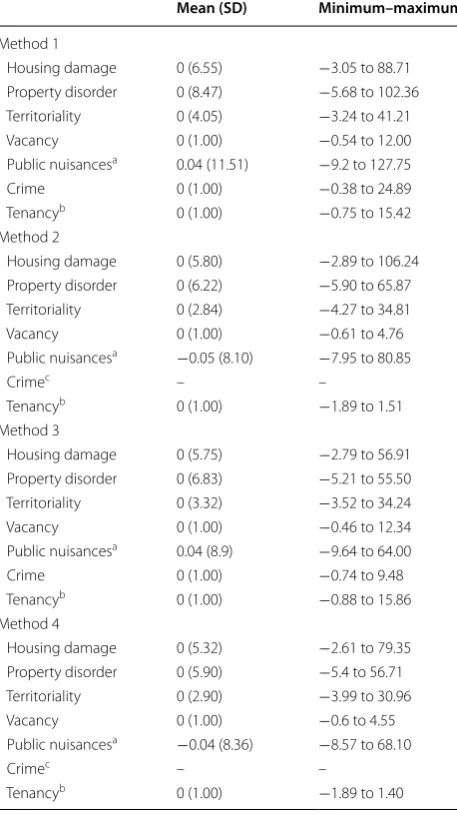
The mean, SD, minimum, and maximum of the seven BE indices for each construction method are presented in Table 2. Among the four BE indices made up of more than one variable (housing damage, property disorder, territoriality, and public nuisances), Method 1, which was based on a simple count, resulted in the largest variation. Variation in indices constructed using Method 3, which accounted for parcel area, was greater than variation in indices constructed using Method 2, which accounted for number of parcels, with the exception of housing damage. Variation based on Method 4 was index specific. Crime
Table 1 Definitions of alternative construction methods for one variable
For example, security bars is one variable that contributes to the territoriality index. Additional file 1: Table S1 details which variables contribute to each index
Method Definition
Method 1 Count of parcels with variable present Method 2 Count of parcels with variable present
Total number of parcels Method 3 Count of parcels with variable present
Total area
measures constructed from a simple count (Method 1) resulted in a larger range than those standardized by area (Method 3), while the range of vacancy and tenancy was greatest when constructed using Methods 1 or 3.
Correlations among alternatively-constructed meas-ures of the same index are presented in Table 3. Con-sistent with previous research [33–35], we used the following categories to evaluate rank preservation: a
correlation ≥0.7 indicated a well preserved index, a cor-relation ≥0.5 and <0.7 indicated a moderately preserved index, a correlation ≥0.3 to <0.5 indicated a weakly pre-served index, and a correlation <0.3 indicated a very weakly or not preserved index. We observe that housing damage, property disorder, vacancy, and crime were well preserved across Methods 1–4 (ρ = 0.91–0.98, 0.77–0.94, 0.89–0.96, and 0.78, respectively), while territoriality
Table 2 Summary statistics of the seven built environment indices by method, census block level, 2011 (N = 1380)
Method 1 is a simple count, Method 2 is an average count per parcel, Method 3 is an average count per unit area, and Method 4 is proportion of area with a variable present
SD standard deviation
a N for public nuisances is 1356 due to data availability
b N for tenancy is 1358 due to data availability
c Crime is not constructed using Methods 2 or 4 as crime is measured at the
block level
Mean (SD) Minimum–maximum
Method 1
Housing damage 0 (6.55) −3.05 to 88.71 Property disorder 0 (8.47) −5.68 to 102.36 Territoriality 0 (4.05) −3.24 to 41.21 Vacancy 0 (1.00) −0.54 to 12.00 Public nuisancesa 0.04 (11.51) −9.2 to 127.75
Crime 0 (1.00) −0.38 to 24.89 Tenancyb 0 (1.00) −0.75 to 15.42
Method 2
Housing damage 0 (5.80) −2.89 to 106.24 Property disorder 0 (6.22) −5.90 to 65.87 Territoriality 0 (2.84) −4.27 to 34.81 Vacancy 0 (1.00) −0.61 to 4.76 Public nuisancesa −0.05 (8.10) −7.95 to 80.85
Crimec – –
Tenancyb 0 (1.00) −1.89 to 1.51
Method 3
Housing damage 0 (5.75) −2.79 to 56.91 Property disorder 0 (6.83) −5.21 to 55.50 Territoriality 0 (3.32) −3.52 to 34.24 Vacancy 0 (1.00) −0.46 to 12.34 Public nuisancesa 0.04 (8.9) −9.64 to 64.00
Crime 0 (1.00) −0.74 to 9.48 Tenancyb 0 (1.00) −0.88 to 15.86
Method 4
Housing damage 0 (5.32) −2.61 to 79.35 Property disorder 0 (5.90) −5.4 to 56.71 Territoriality 0 (2.90) −3.99 to 30.96 Vacancy 0 (1.00) −0.6 to 4.55 Public nuisancesa −0.04 (8.36) −8.57 to 68.10
Crimec – –
Tenancyb 0 (1.00) −1.89 to 1.40
Table 3 Spearman’s correlations between alternatively-constructed measures of each index, census block level, 2011 (N = 1380)
Method 1 is a simple count, Method 2 is an average count per parcel, Method 3 is an average count per unit area, and Method 4 is proportion of area with a variable present
a N for public nuisances is 1356 due to data availability
b Crime is not constructed using Methods 2 or 4 as crime is measured at the
block level
c N for tenancy is 1358 due to data availability
(1) (2) (3) (4)
Housing damage
Method 1 (1) 1.00 0.93 0.92 0.91
Method 2 (2) 1.00 0.97 0.98
Method 3 (3) 1.00 0.96
Method 4 (4) 1.00
Property disorder
Method 1 1.00 0.80 0.79 0.77
Method 2 1.00 0.88 0.94
Method 3 1.00 0.85
Method 4 1.00
Territoriality
Method 1 1.00 0.66 0.61 0.60
Method 2 1.00 0.73 0.90
Method 3 1.00 0.69
Method 4 1.00
Vacancy
Method 1 1.00 0.91 0.89 0.91
Method 2 1.00 0.94 0.96
Method 3 1.00 0.92
Method 4 1.00
Public nuisancesa
Method 1 1.00 0.54 0.80 0.56
Method 2 1.00 0.71 0.94
Method 3 1.00 0.67
Method 4 1.00
Crimeb
Method 1 1.00 – 0.78 –
Method 3 1.00 –
Tenancyc
Method 1 1.00 0.25 0.46 0.26
Method 2 1.00 0.46 0.94
Method 3 1.00 0.36
and public nuisances were moderately to well preserved across methods (ρ = 0.60–0.90 and 0.54–0.94, respec-tively). Preservation of tenancy depended on a given pairwise comparison between methods (ρ = 0.25–0.94). Comparing tenancy constructed using Methods 2 and 4 suggested a well preserved index (ρ = 0.94), while com-paring Methods 1 and 2 or 4 indicated a very weakly preserved index (ρ = 0.25–0.26, respectively). All other pairwise comparisons suggested a weakly preserved index (ρ = 0.36–0.46).
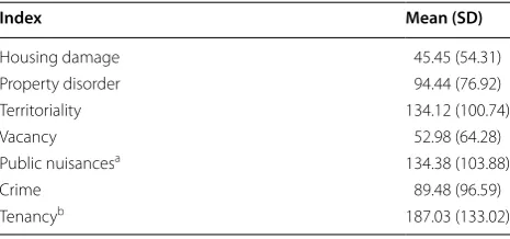
The mean and SD of the average MAD for each BE index are presented in Table 4. Larger means indicate that block rank was more heavily impacted by construc-tion method. Interpreted as the average difference from the mean block rank, the highest average MAD values were for tenancy (mean = 187.03, SD = 133.02), public nuisances (mean = 134.38, SD = 103.88), and territori-ality (mean = 134.12, SD = 100.74). The lowest average MAD values were for housing damage (mean = 45.45, SD = 54.31) and vacancy (mean = 52.98, SD = 64.28). It is important to note that the high MAD values corre-spond to a roughly 14 % difference in ranks; whereas the lowest MAD value corresponds to a roughly 3 % differ-ence in ranks. Figure 3 presents an example of the spatial distribution of MAD using territoriality.
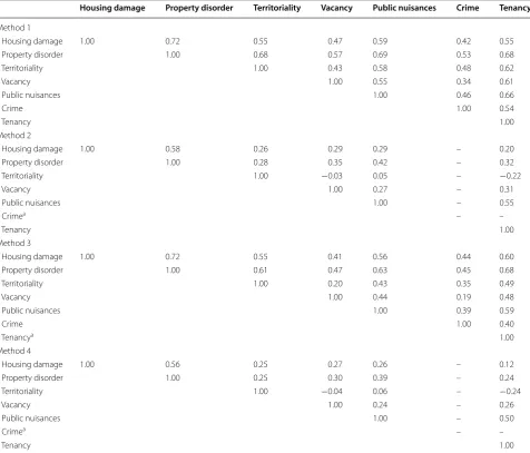
Table 5 presents the correlations among indices for each construction method. Preservation of relationships among different indices (e.g., housing damage and prop-erty disorder) implies similar correlations independent of construction method. Since we are not aware of any a priori defined thresholds for assessing the preservation of a relationship between BE indices across methods, for consistency, we use the same categories as previously mentioned. If the strength of the relationship between two indices varies across Methods 1–4 (e.g., the relation-ship between housing damage and property disorder is weak using Method 1 and moderate using Method 2), the
relationship is considered to be weakly preserved. If the strength of the relationship is consistent across Meth-ods 1–4, it is considered to be well preserved. Correla-tions between crime and housing damage, territoriality, or public nuisances, and public nuisances and tenancy were indicative of well preserved relationships across Methods 1–4, while relationships among all other indi-ces were weakly preserved. For example, the relationship between property disorder and territoriality was very weak using Methods 2 or 4 (ρ = 0.28 and 0.25, respec-tively) and moderate using Methods 1 or 3 (ρ = 0.68 and 0.61, respectively). In general, relationships appeared to be well preserved when comparing indices constructed using Method 2 that accounted for number of parcels to Method 4 that accounted for proportion of the area with a variable present, or Method 1 based on a simple count to Method 3 that accounted for area.
To evaluate whether our findings were consistent across spatial scale, we replicated our analysis at the PAC and SAC levels. Findings were reasonably consist-ent across spatial scale when assessing index-specific preservation across methods for housing damage, terri-toriality, public nuisances, and tenancy (Additional file 1: Tables S2, S3). Crime and vacancy, which were well pre-served across Methods 1–4 at the block level (ρ = 0.78 and 0.89–0.96, respectively), were less preserved at the PAC (ρ = 0.45 and 0.58–0.84, respectively) and SAC lev-els (ρ = 0.29 and 0.54–0.88, respectively). Property dis-order, which was well preserved across Methods 1–4 at the block and PAC levels (ρ = 0.77–0.94 and 0.72–0.90, respectively), was moderately to well preserved at the SAC level (ρ = 0.68–0.93).
Relationships between indices that were preserved across Methods 1–4 at the block level were weakly pre-served across methods at the PAC and SAC levels, while a majority of the relationships that were impacted at the block level remained impacted at the PAC and SAC levels (Additional file 1: Tables S5, S6). We observe that the rela-tionships between housing damage and crime, and public nuisances and tenancy, which were well preserved across methods at the block level (ρ = 0.42–0.44 and 0.50–0.66, respectively), were weakly preserved across methods at the PAC (ρ = 0.40–0.63 and 0.37–0.77, respectively) and SAC levels (ρ = 0.38–0.70 and 0.57–0.87, respec-tively). Further, the relationships between crime and ter-ritoriality or public nuisances were well preserved across methods at the block (ρ = 0.35–0.48 and 0.39–0.46, respectively) and PAC levels (ρ = 0.54–0.64 and 0.60– 0.64, respectively) but weakly preserved at the SAC level (ρ = 0.64–0.70 and 0.63–0.71, respectively). In contrast, the relationships between housing damage and property disorder, and crime and tenancy were weakly preserved across methods at the block level (ρ = 0.58–0.72 and
Table 4 Summary statistics of index-specific mean abso-lute difference (MAD) in rank, census block level, 2011 (N = 1380)
SD standard deviation
a N for public nuisances is 1356 due to data availability
b N for tenancy is 1358 due to data availability
Index Mean (SD)
Housing damage 45.45 (54.31)
Property disorder 94.44 (76.92)
Territoriality 134.12 (100.74)
Vacancy 52.98 (64.28)
Public nuisancesa 134.38 (103.88)
Crime 89.48 (96.59)
0.40–0.54, respectively) but well preserved at the PAC (ρ = 0.75–0.88 and 0.62–0.65, respectively) and SAC lev-els (ρ = 0.84–0.93 and 0.72–0.73, respectively). Similarly, the relationships between vacancy and crime, and prop-erty disorder and territoriality were weakly preserved across methods at the block (ρ = 0.19–0.34 and 0.25– 0.68, respectively) and PAC levels (ρ = 0.49–0.53 and 0.55–0.82, respectively) but well preserved at the SAC level (ρ = 0.54–0.58 and 0.71–0.93, respectively).
Correlations among alternatively-constructed meas-ures of the same index were relatively consistent across
years, as were correlations among indices (Additional file 1: Tables S8, S10, S11, S12).
Discussion
Using objective survey data supplemented with admin-istrative data collected at two time points, we assessed the impact of construction method on the reliability of seven BE indices and evaluated whether findings were consistent across spatial scale. Results indicated that the tenancy index was strongly impacted by construction method at the block level while territoriality and public
Table 5 Spearman’s correlations among indices by method, census block level, 2011 (N = 1380)
Method 1 is a simple count, Method 2 is an average count per parcel, Method 3 is an average count per unit area, and Method 4 is proportion of area with a variable present
N for the pairwise comparison between public nuisances and tenancy is 1336, N for other pairwise comparisons involving public nuisances is 1356, and N for other pairwise comparisons involving tenancy is 1358 due to data availability
a Crime is not constructed using Methods 2 or 4 as crime is measured at the block level
Housing damage Property disorder Territoriality Vacancy Public nuisances Crime Tenancy
Method 1
Housing damage 1.00 0.72 0.55 0.47 0.59 0.42 0.55
Property disorder 1.00 0.68 0.57 0.69 0.53 0.68
Territoriality 1.00 0.43 0.58 0.48 0.62
Vacancy 1.00 0.55 0.34 0.61
Public nuisances 1.00 0.46 0.66
Crime 1.00 0.54
Tenancy 1.00
Method 2
Housing damage 1.00 0.58 0.26 0.29 0.29 – 0.20
Property disorder 1.00 0.28 0.35 0.42 – 0.32
Territoriality 1.00 −0.03 0.05 – −0.22
Vacancy 1.00 0.27 – 0.31
Public nuisances 1.00 – 0.55
Crimea – –
Tenancy 1.00
Method 3
Housing damage 1.00 0.72 0.55 0.41 0.56 0.44 0.60
Property disorder 1.00 0.61 0.47 0.63 0.45 0.68
Territoriality 1.00 0.20 0.43 0.35 0.49
Vacancy 1.00 0.44 0.19 0.48
Public nuisances 1.00 0.39 0.59
Crime 1.00 0.40
Tenancya 1.00
Method 4
Housing damage 1.00 0.56 0.25 0.27 0.26 – 0.12
Property disorder 1.00 0.25 0.30 0.39 – 0.24
Territoriality 1.00 −0.04 0.06 – −0.24
Vacancy 1.00 0.24 – 0.26
Public nuisances 1.00 – 0.50
Crimea – –
nuisances indices were moderately impacted. Excluding the relationships between crime and housing damage, territoriality, or public nuisances, and tenancy and public nuisances, relationships among BE indices were impacted by construction method. Extending the block to account for nearby areas, the number of indices impacted by con-struction method increased as spatial scale increased. Findings involving vacancy, crime, and property dis-order were modified at the PAC and SAC levels, often becoming less preserved with increasing spatial scale. Relationships among indices were consistently impacted by construction method across spatial scale or became impacted as spatial scale increased with a few exceptions. The relationships between crime and vacancy or tenancy, and property disorder and housing damage or territorial-ity appeared to be less impacted by construction method as spatial scale increased.
We found that the impact of construction method on measures of the BE was not only index and spatial scale specific but also depended on which methods we were comparing. These findings are in line with previous research that suggested that the strength of the relation-ship between alternatively-constructed measures of the food environment depended on the approaches being compared [27]. Additionally, research has demonstrated that methodological decisions such as buffer size affect measures of access to green space or public open space, walkability, and other land use characteristics [25, 36, 37]. Such sensitivity is consequential to using BE indices in applied research. For example, when using a data reduc-tion technique like principal components analysis that relies on the correlation structure to summarize informa-tion, construction method and spatial scale may lead to a different number of composite indices, either consist-ent with a priori hypotheses or not. In turn, associations between BE and health outcomes may be affected.
Our research indicates that how well relationships were preserved varied according to index and spatial scale. Territoriality, public nuisances, and tenancy indices were less well preserved than other indices at the block level. These findings can be ascribed to how often ables contributing to an index were observed and vari-ation in area and number of parcels. As varivari-ation in the count of a variable (i.e., graffiti), area, and number of par-cels across the study area increases, block rank becomes less preserved. Alternatively, as variation in the count of a variable, area, or number of parcels across the study area decreases, block rank becomes well preserved as all counts of a variable are divided by the same area or num-ber of parcels. Fencing and security signs from the terri-toriality index, food garbage, cigarettes, broken glass, and high weeds from the public nuisances index, and renter-occupied parcels from the tenancy index were observed
more often than variables contributing to the prop-erty disorder and housing damage indices. Further, we observed variation in area and number of parcels across the study area. Thus, adjusting block-level counts of ter-ritoriality, public nuisances, and tenancy variables by the number of parcels or area impacted the index and corre-sponding block rank more than that of property disorder and housing damage. This can be seen in Table 4, which shows that MAD is highest for territoriality, public nui-sances, and tenancy.
Further, we found that index preservation was spatial scale specific. At the block level, only three indices were affected by construction method while two and three additional indices were also affected at the PAC and SAC levels, respectively. Variation in index preservation across spatial scale is likely driven by relative dissimilar-ity among neighboring units. For example, crime, which appeared reliable at the block level (ρ = 0.78), was less reliable at the PAC and SAC levels (ρ = 0.45 and 0.29, respectively), indicating that as spatial scale increased, the difference in crime measures due to construction method increased in magnitude. Research suggests that crime is clustered, with areas of high crime in close prox-imity to areas of low crime [38]. Consequently, account-ing for crime and area in adjacent blocks, as PAC and SAC level measures do, can significantly impact the rank of a given block, with the magnitude depending on how dissimilar nearby blocks are. Further, heteroge-neity among neighboring units can explain why certain relationships among indices were affected differentially across spatial scale. Accounting for adjacent blocks affected index-specific block rank which, in turn, affected relationships among indices.
This has implications when deciding upon construction methods to formulate and perform sensitivity analysis. Researchers should consider the underlying geography of the study area, as this may shed light on observed asso-ciations with health outcomes. Further, operationalizing measures for the main analysis and sensitivity analysis using formulations that result in less similar measures (e.g., comparing Methods 2 and 3 or comparing Meth-ods 1 and 4) may provide additional insights about the robustness of the study findings.
Our study contains important limitations. First, we assumed that variables within each index contribute equally, which may influence BE indices if at least one of the variables disproportionately influences the index environment more than other variables (e.g., barbed wire impacts the territoriality index more than security signs). Alternative weighting schemes, for example based on the proportion of events of a variable in a census block, may alter block ranks and consequently findings related to reliability. Second, since there is no precedence for evalu-ating the impact of construction method on relationships among different indices, we used an exploratory approach based on Spearman’s correlations. However, as research on the implications of methodological choice develops, more rigorous methods that are conducive to the case of simultaneously evaluating multiple indices may emerge. Third, while our categories of strength of preservation are admittedly arbitrary, we sought to be consistent with previous research assessing index reliability. Fourth, we strove to understand the effect of methodological het-erogeneity on objective measures of the BE. Measures derived from resident surveys on neighborhood percep-tion (i.e., how individuals perceive their environment), which research suggests may be meaningful to health outcomes [39–41], may result in alternative findings pertaining to reliability. Further, perceptive measures of the BE may more accurately measure the BE that affects a person’s health, as the definition of “neighborhood” is sometimes decided by the interviewee. Fifth, similari-ties among indices and relationships among indices con-structed using Methods 1 and 3, and Methods 2 and 4, are at least partially dependent on characteristics of our study area. Data were collected in a densely populated and urban area, where area was somewhat consistent across blocks in the study area and each block contained similarly-sized parcels. Consequently, certain indices and relationships among indices constructed using Methods 1 and 3, and Methods 2 and 4, were similar. We anticipate that our results are likely robust to other urban areas but less likely to be similar to suburban and rural areas where blocks and parcels within each block are less similar in size. Finally, as data were collected in a mid-sized city
located in the southeastern United States, our study may not be generalizable to ultra-dense BEs like Hong Kong, Beijing, or Mumbai [42, 43]. For example, in such envi-ronments, standardizing by some measure of dwelling density may be more appropriate than a simple measure of geographic area. Moreover, the reliability of indices in ultra-dense BEs may be especially sensitive to spatial scale due to the presence of increased geographic hetero-geneity. More research is needed in this area.
Conclusions
To our knowledge, this is the first study to respond to researchers’ calls for a systematic assessment of the impact of methodological choice on BE indices in the areas of construction method and spatial scale [12, 14–
16]. In particular, using a parcel-level objective survey on the BE, we demonstrate that (1) reliability of BE indices is sensitive to construction method and spatial scale; and (2) given the index-specific variation that we observed, evaluation needs to take place on a case-by-case basis. The underlying geography of the study area, character-ized in our study according to the number of parcels and the geographic area, determines whether the potential to observe BE variables is uniform across spatial units. Varying potential for observation, for example according to the number of parcels within census blocks across the study area, translates to increased sensitivity of reliabil-ity to construction method. Spatial scale of measurement may be particularly important to reliability in study areas with highly heterogeneous BEs [44, 45]. In the absence of an a priori reason to choose a certain BE construc-tion method, examining alternative construcconstruc-tions of BE indices, while carefully considering methodological assumptions, may provide insight into features of local geography driving analytical findings.
Abbreviations
BE: built environment; GIS: geographic information system; CAP: Community Assessment Project; PAC: primary adjacency community; SAC: secondary adja-cency community; IRR: inter-rater reliability; MAD: mean absolute difference; SD: standard deviation.
Authors’ contributions
JS led the analysis and contributed to manuscript preparation. RA oversaw the analysis, reviewed analytical results, and contributed to manuscript preparation. MLM conceived the study, reviewed analytical results, and con-tributed to manuscript preparation. All authors read and approved the final manuscript.
Author details
1 School of Natural Resources and the Environment, University of Michigan,
Ann Arbor, MI 48109, USA. 2 Children’s Environmental Health Initiative, Rice
University, Houston, TX 77005, USA. 3 Department of Statistics, Rice University,
6100 Main Street, MS-2, Houston, TX 77005, USA. 4 Department of Pediatrics,
University of Michigan, Ann Arbor, MI 48109, USA. 5 Department of Pediatrics,
Baylor College of Medicine, Houston, TX 77030, USA. 6 Department of
Pediat-rics, Duke University, Durham, NC 27708, USA.
Acknowledgements
We gratefully acknowledge Ruiyang Li for creating maps, and Joshua Tootoo, Mercedes Bravo, and Gretchen Kroeger for providing critical feedback during the manuscript development.
Competing interests
The authors declare that they have no competing interests.
Funding
This work was supported through a grant from the US Environmental Protec-tion Agency (RD-83329301).
Received: 21 January 2016 Accepted: 18 April 2016
References
1. Roof K, Oleru N. Public health: Seattle and King County’s push for the built environment. J Environ Health. 2008;71(1):24–7.
2. Miranda ML, Messer LC, Kroeger GL. Associations between the quality of the residential built environment and pregnancy outcomes among women in North Carolina. Environ Health Perspect. 2012;120(3):471–7. 3. Ochodo C, Ndetei DM, Moturi WN, Otieno JO. External built residential environment characteristics that affect mental health of adults. J Urban Health. 2014;91(5):908–27.
4. Messer LC, Maxson P, Miranda ML. The urban built environment and associations with women’s psychosocial health. J Urban Health. 2013;90(5):857–71.
5. Galea S, Ahern J, Rudenstine S, Wallace Z, Vlahov D. Urban built environ-ment and depression: a multilevel analysis. J Epidemiol Community Health. 2005;59(10):822–7.
6. Weich S, Blanchard M, Prince M, Burton E, Erens B, Sproston K. Mental health and the built environment: cross-sectional survey of individual and contextual risk factors for depression. Br J Psychiatry. 2002;180:428–33. 7. Francis J, Wood LJ, Knuiman M, Giles-Corti B. Quality or quantity?
Explor-ing the relationship between public open space attributes and mental health in Perth, Western Australia. Soc Sci Med. 2012;74(10):1570–7. Additional files
Additional file 1. Community Assessment Project (CAP) variables and PAC, SAC, and 2008 results.
Additional file 2. R code for constructing PACs and SACs from a shapefile.
8. Gordon-Larsen P, Nelson MC, Page P, Popkin BM. Inequality in the built environment underlies key health disparities in physical activity and obesity. Pediatrics. 2006;117(2):417–24.
9. Miranda ML, Edwards SE, Anthopolos R, Dolinsky DH, Kemper AR. The built environment and childhood obesity in Durham, North Carolina. Clin Pediatr. 2012;51(8):750–8.
10. Curtis LJ, Dooley MD, Phipps SA. Child well-being and neighbourhood quality: evidence from the Canadian National Longitudinal Survey of Children and Youth. Soc Sci Med. 2004;58(10):1917–27.
11. Kohen DE, Brooks-Gunn J, Leventhal T, Hertzman C. Neighborhood income and physical and social disorder in Canada: associations with young children’s competencies. Child Dev. 2002;73(6):1844–60. 12. Feng J, Glass TA, Curriero FC, Stewart WF, Schwartz BS. The built
environ-ment and obesity: a systematic review of the epidemiologic evidence. Health Place. 2010;16(2):175–90.
13. Casey R, Oppert J-M, Weber C, Charreire H, Salze P, Badariotti D, Banos A, Fischler C, Hernandez CG, Chaix B. Determinants of childhood obesity: what can we learn from built environment studies? Food Qual Prefer. 2014;31:164–72.
14. Rollings KA, Wells NM, Evans GW. Measuring physical neighborhood qual-ity related to health. Behav Sci. 2015;5(2):190–202.
15. Schaefer-McDaniel N, Dunn JR, Minian N, Katz D. Rethinking measure-ment of neighborhood in the context of health research. Soc Sci Med. 2010;71(4):651–6.
16. Ding D, Gebel K. Built environment, physical activity, and obesity: what have we learned from reviewing the literature? Health Place. 2012;18(1):100–5.
17. McGinn AP, Evenson KR, Herring AH, Huston SL, Rodriguez DA. Exploring associations between physical activity and perceived and objective measures of the built environment. J Urban Health. 2007;84(2):162–84.
18. Leonard TC, Caughy MO, Mays JK, Murdoch JC. Systematic neighborhood observations at high spatial resolution: methodology and assessment of potential benefits. PLoS One. 2011;6(6):e20225.
19. Colabianchi N, Coulton CJ, Hibbert JD, McClure SM, Ievers-Landis CE, Davis EM. Adolescent self-defined neighborhoods and activity spaces: spatial overlap and relations to physical activity and obesity. Health Place. 2014;27:22–9.
20. Ding D, Sallis JF, Kerr J, Lee S, Rosenberg DE. Neighborhood environ-ment and physical activity among youth a review. Am J Prev Med. 2011;41(4):442–55.
21. Schaefer-McDaniel N, Caughy MO, O’Campo P, Gearey W. Examining methodological details of neighbourhood observations and the relation-ship to health: a literature review. Soc Sci Med. 2010;70(2):277–92. 22. James P, Berrigan D, Hart JE, Hipp JA, Hoehner CM, Kerr J, Major JM, Oka
M, Laden F. Effects of buffer size and shape on associations between the built environment and energy balance. Health Place. 2014;27:162–70. 23. Boone-Heinonen J, Popkin BM, Song Y, Gordon-Larsen P. What
neighbor-hood area captures built environment features related to adolescent physical activity? Health Place. 2010;16(6):1280–6.
24. Brew J. (Mis)measurement in the study of food environment: we need better methods to solve the puzzle. J Epidemiol Community Health. 2015;69(8):817–8.
25. Higgs G, Fry R, Langford M. Investigating the implications of using alternative GIS-based techniques to measure accessibility to green space. Environ Plan Part B. 2012;39(2):326.
26. Villanueva K, Badland H, Hooper P, Koohsari MJ, Mavoa S, Davern M, Roberts R, Goldfeld S, Giles-Corti B. Developing indicators of public open space to promote health and wellbeing in communities. Appl Geogr. 2015;57:112–9.
27. Burgoine T, Alvanides S, Lake AA. Creating ‘obesogenic realities’; do our methodological choices make a difference when measuring the food environment? Int J Health Geogr. 2013;12:33.
28. Kroeger GL, Messer L, Edwards SE, Miranda ML. A novel tool for assessing and summarizing the built environment. Int J Health Geogr. 2012;11:46. 29. Caughy MO, O’Campo PJ, Patterson J. A brief observational measure for
urban neighborhoods. Health Place. 2001;7(3):225–36.
• We accept pre-submission inquiries
• Our selector tool helps you to find the most relevant journal • We provide round the clock customer support
• Convenient online submission • Thorough peer review
• Inclusion in PubMed and all major indexing services • Maximum visibility for your research
Submit your manuscript at www.biomedcentral.com/submit
Submit your next manuscript to BioMed Central
and we will help you at every step:
31. Radenbush S, Sampson R. Econometrics: toward a science of assessing ecological settings, with application to the systematic social observation of neighbourhoods. Sociol Methodol. 1999;29:1–41.
32. Landis JR, Koch GG. The measurement of observer agreement for cat-egorical data. Biometrics. 1977;33(1):159–74.
33. Tyrakowski M, Mardjetko S, Siemionow K. Radiographic spinopelvic parameters in skeletally mature patients with Scheuermann disease. Spine. 2014;39(18):E1080–5.
34. Stanton R, Reaburn P, Happell B. Barriers to exercise prescription and participation in people with mental illness: the perspectives of nurses working in mental health. J Psychiatr Ment Health Nurs. 2015;22(6):440–8. 35. Mukaka MM. Statistics corner: a guide to appropriate use of correlation
coefficient in medical research. Malawi Med J. 2012;24(3):69–71. 36. Yamada I, Brown BB, Smith KR, Zick CD, Kowaleski-Jones L, Fan JX. Mixed
land use and obesity: an empirical comparison of alternative land use measures and geographic scales. Prof Geogr. 2012;64(2):157–77. 37. Brown BB, Yamada I, Smith KR, Zick CD, Kowaleski-Jones L, Fan JX.
Mixed land use and walkability: variations in land use measures and relationships with BMI, overweight, and obesity. Health Place. 2009;15(4):1130–41.
38. Andresen MA. Estimating the probability of local crime clus-ters: the impact of immediate spatial neighbors. J Crim Justice. 2011;39(5):394–404.
39. Peachey AA, Baller SL. Perceived built environment characteristics of on-campus and off-on-campus neighborhoods associated with physical activity of college students. J Am Coll Health. 2015;63(5):337–42.
40. Booth ML, Owen N, Bauman A, Clavisi O, Leslie E. Social–cognitive and perceived environment influences associated with physical activity in older Australians. Prev Med. 2000;31(1):15–22.
41. Humpel N, Owen N, Leslie E, Marshall AL, Bauman AE, Sallis JF. Associa-tions of location and perceived environmental attributes with walking in neighborhoods. Am J Health Promot. 2004;18(3):239–42.
42. Cerin E, Chan K, Macfarlane DJ, Lee K, Lai P. Objective assessment of walk-ing environments in ultra-dense cities: development and reliability of the environment in Asia scan tool—Hong Kong version (EAST-HK). Health Place. 2011;17(4):937–45.
43. Alfonzo M, Guo Z, Lin L, Day K. Walking, obesity and urban design in Chinese neighborhoods. Prev Med. 2014;69:S79–85.
44. Haynes R, Jones AP, Reading R, Daras K, Emond A. Neighbourhood vari-ations in child accidents and related child and maternal characteristics: does area definition make a difference? Health Place. 2008;14(4):693–701. 45. Haynes R, Daras K, Reading R, Jones A. Modifiable neighbourhood units,