R E S E A R C H A R T I C L E
Open Access
Stratification of earth’s outermost core
inferred from SmKS array data
Satoshi Kaneshima
1*and Takanori Matsuzawa
2Abstract
SmKS arrivals recorded by large-scale broadband seismometer arrays are analyzed to investigate the depth profile of P wave speed (Vp) in the outermost core. TheVp structure of the upper 700 km of the outer core has been
determined using SmKS waves of Fiji-Tonga events recorded at stations in Europe. According to a recent outer core model (KHOMC), theVp value is 0.45 % slower at the core mantle boundary (CMB) than produced by the Preliminary Reference Earth Model (PREM), and the slow anomaly gradually diminishes to insignificant values at∼300 km below the CMB. In this study, after verifying these KHOMC features, we show that the differential travel times measured for SmKS waves that are recorded by other large-scale arrays sampling laterally different regions are well matched by KHOMC. We also show that KHOMC precisely fits the observed relative slowness values between S2KS, S3KS, and S4KS (SmKS waves withm=2, 3, and 4). Based on these observations, we conclude that SmKS predominantly reflect the outer core structure. Then we evaluate biases of secondary importance which may be caused by mantle
heterogeneity. The KHOMCVp profile can be characterized by a significant difference in the radialVp gradient between the shallower 300 km and the deeper part of the upper 700 km of the core. The shallower part has a Vp gradient of−0.0018s−1, which is steeper by 0.0001s−1when compared to the deeper core presented by PREM. The steeperVp gradient anomaly of the uppermost core corresponds to a radial variation in the pressure derivative of the bulk modulus,K=dK/dP. TheKvalue is 3.7, which is larger by about 0.2 than that of the deeper core. The radial variation inKis too large to have a purely thermal origin, according to recent ab initio calculations on liquid iron alloys, and thus requires a thick and compositionally stratified layering at the outermost outer core.
Keywords: Outermost core; Compositional stratification; SmKS waves; Array processing
Background
Stratification of the outermost core has been long sus-pected (e.g., Lay and Young 1990; Buffett and Seagle 2010) and has been recently strongly advocated by Helffrich and Kaneshima (2010) and Kaneshima and Helffrich (2013) (respectively abbreviated as HK2010 and KH2013 here-after). The present study consolidates the propositions of HK2010 and KH2013 by investigating additional SmKS data obtained for significantly more event-array pairs and by evaluating possible mantle effects on SmKS travel time and slowness observations. We analyze SmKS arrivals with integermfrom 2 to 5 in order to better constrain the Vp profile of the topmost 700 km of the core, anticipating
*Correspondence: [email protected]
1Department of Earth and Planetary Science, Kyushu University, Hakozaki, Higashi-ku, 812-8581 Fukuoka, Fukuoka, Japan
Full list of author information is available at the end of the article
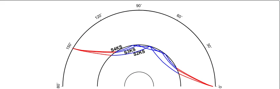
that the results will strengthen the evidence for a compo-sitionally stratified layer. As shown in Fig. 1, the ray paths of S2KS, S3KS, and S4KS propagate quite a long distance through the outermost part of the core. Since each SmKS possesses a distinct depth sensitivity depending both onm and epicentral distance, when used in combination, SmKS waves can form an ideal data set for use in determining the Vp profile of the outermost core. In order to measure dif-ferential travel time and slowness differences between two SmKS waves, we used large-scale broadband seismome-ter arrays in Europe, Easseismome-tern Asia (including Japan), North and South America, Africa, and Australia.
Prior to HK2010 and KH2013, other studies also inves-tigated the outer core structure by analyzing SmKS data. The proposed models show either slightly or rather strongly slower Vp anomaly relative to the Prelimi-nary Reference Earth Model (PREM) (Dziewonski and Anderson 1981) near the top of the core. For instance,
Fig. 1SmKS ray paths. Ray paths of SmKS waves (S2KS, S3KS, and S4KS) propagating through the outermost part of the core to a receiver at a epicentral distance of 150°. Blue and red lines show P and S wave portions of the rays, respectively
Tanaka (2007) analyzed a composite record section of S2KS, S3KS, and S4KS, which were observed globally, and proposed a model with up to a maximum of 1.2 % slowerVpthan PREM in the outermost 90 km of the core. His model (called Tanaka-1 hereafter) is similar to that presented in an earlier study by Garnero et al. (1993). Alexandrakis and Eaton (2010) investigated composite globally observed record sections of S2KS to S4KS for the distance range shorter than 140° and showed a permissible range ofVpprofiles for the top 200 km of the outer core. The range of permissible models centers around slightly slowerVpvalues (from∼0.1 to 0.4 %) than PREM and falls between PREM and the IASP91 velocity model (Kennett and Engdahl 1991). In this study, we also include other globalVp models such as SP6 (Morelli and Dziewonski 2012), AK135 (Kennett et al. 1995), and another model proposed by Tanaka (2007) (called Tanaka-3 hereafter) with the models to be compared.
SmKS waveform data
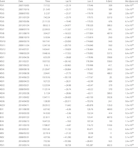
SmKS data are analyzed for earthquakes that occurred in several different regions and were recorded at large-scale broadband stations prior to July 2014 (Table 1). The broadband seismograms in Europe are extracted from the Incorporated Research Institutions for Seismology (IRIS) and the Observatories and Research Facilities for European Seismology (ORFEUS) data management cen-ters. Seismic stations in Japan belong to J-Array, F-net, and the tilt-meter network of Hi-net (Obara et al. 2005). Data of the seismic stations in Eastern Asia outside of Japan, the US, and Australia are extracted from the IRIS data management center (DMC). In this study, we loosely define a “large-scale array” as a group of 20 or more broad-band seismometer stations with aperture lengths exceed-ing ∼1000 km whose seismograms can be analyzed by standard array processing methods. As we shall show later, travel times of SmKS waves observed at individual stations
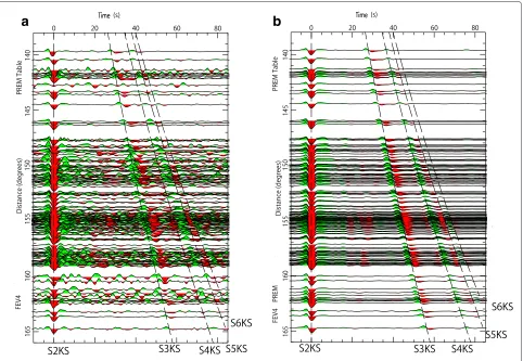
may be significantly affected by the heterogeneous mantle structure, rather irrespective of the waveform quality. This makes it difficult to investigate a detailedVp profile of the outer core based on SmKS measurements made for individual traces. However, HK2010 and KH2013 showed that stacking seismograms over an entire large-scale array substantially suppresses the mantle effects and thereby enables us to discern the fine structure of the outermost core. In this study, we shall also show that the processing of large-scale array data enables us to precisely retrieve differential slowness between two SmKS arrivals, which helps to better constrain the outer core structure. Figure 2 shows an example of observed and computed record sections for a Fiji-Tonga event recorded at the European stations. The synthetic seismograms shown in Fig. 2b are computed for PREM using reflectivity (Kind 1979) and a method similar to that of Wang et al. (2008) (HK2010). When SmKS touches an internal caustic and is underside reflectedm−1 times at the core mantle boundary (CMB), it suffers from a phase delay by nearly m−21π relative to SKS (Choy 1977). The arrivals of S2KS, S3KS, S4KS, S5KS, and S6KS are clearly visible on this section and are sys-tematically delayed with respect to the theoretical PREM predictions throughout the array.
Methods and results Array measurements
Table 1Event list
Event Date Time Lat. N Lon. E h (km) Mo (dyne cm)
FEV1 2007/10/05 7:17:52 −25.19 179.46 509 6.8×1025
FEV2 2007/10/16 21: 5:43 −25.77 179.53 509 1.0×1026
FEV3 2008/07/03 3: 2:37 −23.37 −179.78 581 2.8×1025
FEV4 2011/07/29 7:42:24 −23.79 179.75 537.0 1.5×1026
FEV5 2007/05/06 21:11:53 −19.40 −179.35 676 6.1×1025
FEV6 2012/01/24 00:52: 5 −24.977 178.520 580.3 4.2×1025
FEV7 2008/07/19 22:39:53 −17.337 −177.312 391. 5.2×1025
FEV8 2011/08/19 3:54:27 −16.522 −177.004 407.9 2.9×1025
FEV9 2008/10/19 5:10:34 −21.863 −173.819 29.0 2.9×1026
FEV10 2009/03/19 18:17:41 −23.050 −174.660 34.0 3.4×1027
FEV11 2009/11/24 12:47:16 −20.710 −174.040 18.0 1.7×1026
FEV12 2014/07/21 14:54:41 −19.829 −178.464 616. 3.0×1026
FEV13 1998/03/29 19:48:16 −17.552 −179.092 537.5 6.4×1026
KEV1 2013/04/26 6:53:29 −28.68 −178.96 358.8 2.1×1025
KEV2 2011/02/21 10:57:52 −26.142 178.394 558.0 7.9×1025
KEV3 2007/09/25 5:16: 1 −30.965 179.998 417. 2.3×1025
KEV4 2009/08/18 21:20:47 −26.064 −178.391 269.3 3.6×1025
KEV5 2013/08/28 2:54:41 −27.75 179.62 480.3 2.9×1025
KEV6 2014/06/23 19:19:16 −30.118 −177.67 20. 2.6×1026
AEV1 2000/04/23 9:27:23 −28.31 −62.99 609 3.1×1026
AEV2 2005/03/21 12:23:54 −24.98 −63.47 579 2.3×1026
AEV3 2008/09/03 11:25:14 −26.74 −63.22 570 3.3×1025
AEV4 2012/05/28 5: 7:24 −28.06 −63.11 589.3 1.3×1026
AEV5 2011/09/02 13:47:11 −28.420 −63.150 592.8 1.4×1026
AEV6 2014/04/03 1:58:30 −20.311 −70.576 24.1 9.6×1025
NCEV 2014/04/11 20:29:12 11.642 −85.878 135.0 1.0×1025
IEV1 2011/08/30 6:57:42 −6.36 126.76 469.0 2.7×1026
IEV2 2010/03/20 14: 0:50 −3.36 152.24 414 9.2×1025
IEV3 2010/07/23 22: 8:11 6.72 123.41 607.0 1.2×1027
IEV4 2013/06/13 16:47:23 −10.0 107.24 9.0 1.1×1026
IEV5 2011/03/10 17:08:37 −6.87 116.72 510.6 9.7×1025
IEV6 2010/05/31 19:51:45 11.132 93.471 112. 6.4×1025
MEV 2006/02/22 22:19: 8 −21.32 33.58 11 4.2×1026
INEV 2008/05/31 4:37:56 −41.290 80.47 10. 5.1×1025
SEV1 2014/06/29 7:52:56 −55.506 −28.451 16.5 2.4×1026
PEV1 2013/05/14 0:32:26 18.728 145.287 602.3 2.1×1026
the source time function, which may cause some biases to thedtm−n(differential travel times between SmKS and SnKS waves) and their anomalies relative to ray theo-retical predictions by PREM, which are usually positive. Those biases are mostly less than 0.2 s for the Fiji-Tonga events used in HK2010 and KH2013 but can be larger for other events. Therefore, we evaluate biases by using syn-thetic seismograms (Fig. 2b). To measure these synsyn-thetic
seismogramsdtm−n, we use the same array method as the data and compare them with the theoretical ray calcula-tions based on PREM. The difference, which is usually 0.2 to 0.3 s but sometimes could exceed 0.5 s (Table 2), is regarded as the bias. For each event,dt3−2 are
a
b
Fig. 2Observed and synthetic record sections. The observed (a) and computed (b) record sections of a Fiji-Tonga event recorded at the European stations. The arrivals of S2KS, S3KS, S4KS, S5KS, and S6KS are clearly visible. When aligned on S3KS arrivals, S4KS and S5KS waves are systematically delayed relative to PREM across the entire array. In this example,dt3−2,dt4−3, anddt5−3are anomalous by about +1.2 s
used as the alignment phase whenever the S3KS arrival is sufficiently clear, and the agreements between different alignment phases (S2KS or S3KS) and between differ-ent methods (peak-picking or cross correlating) are used for evaluating the error of eachdt3−2measurement. The measured differential times are classified into two cate-gories, A (high quality) and B (moderate) (Table 2). When the values obtained by different methods agree with each other, the stacked synthetic and observed seismograms usually agree quite well, and the measurements can be regarded as category A, and have smaller errors.
In addition to the π2 phase shift, waveforms of S4KS could be distorted by the interference by S5KS (Eaton and Kendall 2006) or by S3KS when epicentral distances are not large. The S5KS arrivals are not separated com-pletely from S4KS, even when its peak, which is oppositely polarized to S3KS, can be clearly identified. Therefore, dt4−3anddt5−3are measured simply by identifying the corresponding peaks. Since alignment on S4KS arrivals is usually unstable, differential times between S4KS and S5KS (called dt5−4) are calculated by subtracting dt4−3
fromdt5−3with error propagation. Other array
measure-ment details are described in HK2010 and KH2013. We note that, especially for the Tonga-Fiji events (Fig. 2a), the anomalies of dtm−n relative to PREM are observed more or less uniformly across the entire European array (KH2013). Except for the uniform delays, no systematic trends in the differential times with azimuth from the Tonga-Fiji events, which may be amenable to elaborate modeling, have been identified for the high quality events. This would suggest only minor influences of CMB struc-ture on individual paths.
Vpmodel for the outermost core τ−p inversion: effects of starting model
KH2013 built aVp model of the topmost 700 km of the outer core using differential SmKS travel time anomalies of several Fiji-Tonga events recorded at Europe, dt3−2, dt4−3, anddt5−3, to which aτ−pinversion method had
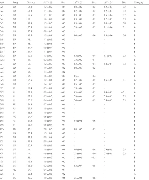
Table 2Differential travel times are measured on the waveforms which are obtained by linearly stacking the observed broadband seismograms with the relative slowness computed for PREM
Event Array Distance dt3−2(s) Bias dt4−3(s) Bias dt5−3(s) Bias Category
FEV1 EU 154.0 1.2±0.2 0.1 1.0±0.2 0.2 1.2±0.3 0.2 A
FEV2 EU 154.0 1.1±0.2 0.2 1.2±0.2 0.2 1.2±0.3 0.3 A
FEV3 EU 152.5 1.1±0.3 0.1 1.3±0.3 0.3 1.5±0.4 0.2 A
FEV4 EU 152. 1.6±0.2 0.2 1.3±0.2 0.2 1.2±0.3 0.3 A
FEV5 EU 147.3 1.5±0.3 0.3 1.3±0.4 0.2 1.6±0.5 0.0 A
FEV6 EU 153.5 1.6±0.4 0.2 0.9±0.2 0.2 1.1±0.4 0.1 A
FEV6 US 123.5 0.9±0.3 0.3 - - B
FEV7 EU 148.5 1.5±0.4 0.3 1.4±0.3 0.4 1.3±0.4 0.4 B
FEV8 EU 148. 1.1±0.5 0.3 - - B
FEV9 EU 153. 1.2±0.5 −0.1 - - B
FEV10 EU 151.9 0.9±0.4 −0.3 - - B
FEV11 EU 151.9 1.1±0.4 0.0 - - B
FEV12 EU 150.0 1.3±0.2 0.3 1.2±0.2 0.4 1.1±0.3 0.3 A
FEV13 AF 131. 0.2±0.3 −0.1 0.2±0.2 −0.1 - B
KEV1 EU 155. 1.2±0.2 0.3 1.2±0.3 0.4 1.0±0.4 0.4 A
KEV2 EU 153. 1.9±0.4 0.2 1.0±0.3 0.2 - B
KEV3 EU 155. 1.4±0.4 0.2 - - B
KEV4 EU 155. 1.6±0.5 0.4 1.5±- 0.4 - B
KEV5 EU 155.5 1.2±0.4 0.3 1.2±0.4 0.2 1.5±0.5 0.1 A
KEV6 EU 155. 1.4±0.3 0.2 1.5±0.5 0.3 - B
AEV1 JP 162.4 0.5±0.4 0.1 0.9±0.4 0.2 - B
AEV2 HI 157.8 0.9±0.4 −0.1 1.3±0.2 0.2 1.4±0.3 −0.1 A
AEV3 HI 162.6 0.5±0.5 0.0 0.9±0.4 0.2 0.8±0.5 0.2 B
AEV4 HI 160.0 0.6±0.3 −0.1 0.6±0.3 0.3 0.5±0.3 0.2 A
AEV4 AU 124.8 0.7±0.3 0.6 - - B
AEV4 AS 167.9 1.0±0.4 0.0 - - B
AEV5 JP 163.4 1.0±0.4 0.0 - - B
AEV5 AU 124.7 0.6±0.4 0.4 - - B
AEV5 AS 167.8 1.0±0.4 0.0 1.4±0.5 0.6 - B
AEV6 JP 153.9 0.6±0.4 −0.1 - - B
NCEV AU 140.1 2.0±0.5 0.7 1.0±0.5 0.3 - B
IEV1 US 130.9 1.3±0.4 0.2 - - B
IEV2 EU 122.8 0.9±0.4 0.1 - - B
IEV2 US 119.5 0.9±0.4 0.1 - - B
IEV3 US 120.9 0.8±0.5 −0.4 - - B
IEV4 US 144. 1.0±0.4 0.4 1.0±0.5 0.4 0.9±0.5 0.5 A
IEV5 US 141. 0.9±0.3 0.1 0.3±0.3 0.0 0.3±0.5 0.2 A
IEV6 US 133.1 0.4±0.2 0.2 0.1±0.3 −0.2 - B
MEV US 149.2 1.0±0.5 0.2 - - B
INEV US 168.6 0.2±0.5 −0.3 1.2±0.4 0.5 - B
SEV1 AK 154.1 0.4±0.5 0.1 - - B
SEV1 JP 153.8 0.9±0.3 0.2 - - A
PEV1 SA 149.5 1.9±0.3 0.5 0.5±0.5 0.6 - B
(Fig. 3). The lower-than PREM Vp values persist down to about 300 km below the CMB. We note here that the
τ −pmethod is a linear inversion that requires a good starting model. Although PREM is known to be a good global model, there may be other reference models as good as PREM. We perform theτ −pinversion using IASP91 as the starting model, as did Alexandrakis and Eaton (2010). By using only the Fiji-Tonga to European stations data, as in the case of KHOMC, we obtained a profile of Vp anomaly relative to IASP91 (called KOCTI). KOCTI has fasterVp values than IASP91 in the shallowest 300 km of the outer core (Fig. 3). KOCTI shows an improved fit to the data compared to IASP91 (Fig. 3), but its over-all fit is less suitable than that of KHOMC, with the most significant disagreement for thedt3−2data of larger dis-tances, as will be shown later in this study. TheVpvalues of KOCTI for the upper 300 km are only about 0.01 km/s slower than those of KHOMC (the Vp at the CMB is−0.045 km/s relative to PREM, while that of KHOMC is−0.035 km/s). Therefore, it can be seen that the two models agree with each other within the uncertainty range (Fig. 3). We conclude that theVp at CMB is constrained well by theτ−pinversion to 8.03±0.01 km/s, irrespective of the starting model. The disagreement between KOCTI and KHOMC for the depth range from about 300 km to 700 km from the CMB is larger (by about −0.02 km/s), suggesting a poorer resolution than the shallower core.
Fig. 3Vp models of outermost core.Vpmodels of the upper 700 km
of the outer core: KHOMC, AK135, SP6, Tanaka-1, Tanaka-3, IASP91, AE09 (Alexandrakis and Eaton 2010), and KOCTI. TheVp values (in
km/s) as a function of depth relative to the PREM values are shown. The uncertainty range of KHOMC are shown in pink (KH2013)
Genetic algorithms
In order to check further the effects of the starting model on the result, we perform another Vp inversion using genetic algorithms (e.g., Yamanaka and Ishida 1995) and attempt to find the global minimum ofdtm−nmisfit in a fashion that does not explicitly require a starting model. TheVp profile of the outer 700 km of the core is assumed to be continuous and consist of four layers with constant Vp gradients. For each layer, theVp value at its top and its thickness are determined (see the caption of Fig. 4 for details).
We use the data set consisting ofdt3−2,dt4−3, anddt5−4 data for four events from Fiji-Tonga to Europe (FEV1, FEV2, FEV3, FEV4) and three events from Argentina to
Fig. 4Genetic algorithm. TheVpmodel obtained by the inversion
using genetic algorithms. The thick black line labeled KOCGA is the obtained continuousVpmodel of the outer 700 km of the core,
which has four layers with uniformVp gradients. Other details are the
same as Fig. 3. The thickness of the deepest layer is fixed to 400 km and theVp value at the bottom of the layer is fixed to that of PREM,
so that there are seven parameters to be determined, each of which is described as a 6-bit binary number. Therefore, each gene has a length of 42 bits. The least bit for theVpat the top of each layer corresponds
to 0.003 km/s, while the least bit for the thickness corresponds to 2 km. The depth of the CMB is fixed to that of PREM, so the inversion is not entirely free from the reference model, but the effect is quite small insofar as the differential travel times of SmKS waves are concerned. The range of theVp value sought by this parameterization
covers about±0.2 km/s relative to PREM, which is wide enough not to miss any successful models. First, the samples ofVp model of the
first generation are constructed by randomly selecting the seven model parameters. Second, the misfit of the model predictions to the observations is computed, and eachVp model sample is selected
Japan (AEV1, AEV2, AEV3) without correcting for bias (Table 2). The inversion is repeated 40 times with dif-ferent initial values, and the case with the least misfit, for which the total residual decreases from 0.5 to 0.15 s through the 40 generations, is chosen. As shown in Fig. 4, the obtained model (called “KOCGA” hereafter) is fairly close to KHOMC. The agreement between the model and KHOMC is remarkable especially for the shallower 300 km of modeled depth range. Based on this result, we con-clude that the validity of KHOMC is not affected by the choice of the starting model.
SmKS slowness measurements
In addition to travel time differences, differences in slow-ness between two SmKS waves provide information on the relative arrival directions of the waves. In HK2010 and KH2013, it was reported that the relative slownesses for the Tonga and Argentina events are close to those predicted by PREM. This observation has been exploited in using the τ-p inversion. The slowness observations can also give constraints on the degree of large-scale heterogeneity in the receiver-side mantle, as shall be shown in the “Discussion” section. The differential slow-ness between two different SmKS waves changes gradually with distance. Therefore, the moveout of a SmSK wave, relative to the reference SmKS wave on a record section, is aligned on a slightly curved line rather than a straight line. Although the curvature is small, when the aperture of an array is as large as 20°, its effect on the differential travel times approaches a second, which could give rise to a small bias of the measured differential slowness between SmKS and SnKS relative to PREM (called “dpm−n”). To ensure thatdpm−nis measured accurately, we correct for the curvature by assuming that the moveout around the array center (distance of 0) is a quadratic function of
epicentral distance when stacking seismograms. Accord-ingly, the differential slowness between S3KS and S2KS (and similarly between S4KS and S2KS) is expressed as
dp3−2()=dp3−2(0)+(−0)
d ddp
3−2
The curvatures of the moveout curve are fixed to those of the reference model, so that dddpis 0.014 and 0.021 s/◦2 for dp3−2 and dp4−2, respectively, which does not
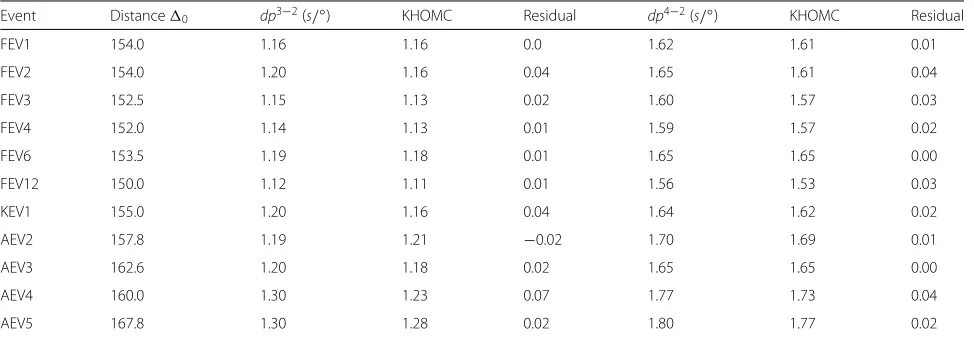
significantly affect the results. We obtain precise slow-ness measurements of S3KS and S4KS waves with S2KS as the reference wave for eight Fiji-Tonga and Kermadec events observed from Europe, and four Argentina events observed from Japan (Table 3). Thedp3−2anddp4−2are then compared to the predictions of KHOMC (Table 3).
Figure 5a shows a vespagram example of the cube-root stack output as a function of slowness and arrival time rel-ative to S2KS, with the small moveout curvature effects corrected. The observed dp3−2 and dp4−2 (red circles)
closely agree with theoretical predictions by KHOMC (Table 3), which are shown by red stars in the figure. The RMS residuals computed for the Fiji-Tonga and Argentina events using the outer core models (PREM, IASP91, KOCTI, AK135, SP6, and Tanaka-1) show that the least residual is obtained for KHOMC (Fig. 5b). The RMS resid-ual is less than 0.03 s/° for KHOMC (Fig. 5b), anddp3−2 for the majority of the events, which agree with KHOMC within 0.02 s/° (Table 3). The residuals for KHOMC of dp3−2anddp4−2are slightly improved in comparison to PREM, while no such dpm−n improvement is seen for the other models. The small discrepancy of the observed dp3−2anddp4−2, with respect to PREM, justifies the usage of PREM as the reference model for stripping the man-tle contributions from the observed distance ranges and travel times in theτ-p inversion that resulted in KHOMC (HK2010; KH2013). While the primary information about the coreVp structure is contained in the differential SmKS travel times, as shown in parameter tests (KH2013), the measured dp3−2 and dp4−2 data not only indicate the
validity of our travel time analyses but also further support the validity of KHOMC.
SmKS differential times of other regions
Observations ofdt3−2
KHOMC was built by using the Tonga-Fiji data set that samples rather limited areas of the CMB, mostly beneath western Pacific and Siberia. KH2013 showed that the SmKS differential travel times of the Argentina to Japan data set are consistent with KHOMC, even though they sample entirely different parts of the CMB. In this study, we compile thedt3−2measurements for additional pairs of event and large-scale array that sample a much larger portion of the CMB. We determine the anomalies ofdt3−2 for several large-scale arrays (Japan, US, Australia, Alaska, Africa, South America, and Southeast Asia; Fig. 6a) using the same processing. The ray paths cover a reasonably large part of the outer core (Fig. 6a).
A striking feature of the result is that thedt3−2
Table 3Differential slowness (dp3-2anddp4-2,s/°)
Event Distance0 dp3−2(s/◦) KHOMC Residual dp4−2(s/◦) KHOMC Residual
FEV1 154.0 1.16 1.16 0.0 1.62 1.61 0.01
FEV2 154.0 1.20 1.16 0.04 1.65 1.61 0.04
FEV3 152.5 1.15 1.13 0.02 1.60 1.57 0.03
FEV4 152.0 1.14 1.13 0.01 1.59 1.57 0.02
FEV6 153.5 1.19 1.18 0.01 1.65 1.65 0.00
FEV12 150.0 1.12 1.11 0.01 1.56 1.53 0.03
KEV1 155.0 1.20 1.16 0.04 1.64 1.62 0.02
AEV2 157.8 1.19 1.21 −0.02 1.70 1.69 0.01
AEV3 162.6 1.20 1.18 0.02 1.65 1.65 0.00
AEV4 160.0 1.30 1.23 0.07 1.77 1.73 0.04
AEV5 167.8 1.30 1.28 0.02 1.80 1.77 0.02
The corresponding values calculated for KHOMC and the residuals of the observed values from the KHOMC predictions are also shown. Alignment is at the center distance of the array
misfit is obtained for KHOMC (Fig. 6c). As mentioned previously, we note that KHOMC definitely gives a bet-ter fit than the τ-p model based on IASP91 (KOCTI) for larger distances. These observations indicate that the mantle effects ondt3−2are of secondary importance and that the essential features of KHOMC relative to PREM reflect the structure of the core.
Observations ofdt4−3anddt5−4
The ray paths for whichdt4−3can be determined by using large-scale array data are geographically more restricted around Pacific than in the case of dt3−2 but still sam-ple a reasonably broad portion of the CMB (Fig. 7a). The measured dt4−3 values fall in the middle of individual station measurements (Garnero et al. 1993) and are well consistent with KHOMC (Fig. 7b). Among theVp mod-els considered (Fig. 7d), thedt4−3 observations are best matched by KOCTI, but the data set (especially for cate-gory A) is explained almost equally well by KHOMC; the dt4−3 data set is not useful for discriminating between the two models. The other models (IASP91, Tanaka-1, Tanaka-3, AK135, and SP6) give significantly poorer fits when compared with KHOMC and KOCTI.
Thedt5−4data set is matched well by some of the
mod-els considered, KHOMC, PREM, IASP91, and KOCTI (Fig. 7c), so that it is not crucial to discriminate between the models. Nevertheless, it clearly refutes the class of models that have a strong Vp reduction in a thin layer at the top of the outer core, such as Tanaka-1, Tanaka-3, and that of Garnero et al. (1993). These models were built without using dt5−4 and were aimed to match mainly dt3−2, which means that the amount ofVpanomaly rela-tive to PREM across the top several hundred kilometers of the outer core can be well predicted by these models. The mismatch between these models with the observeddt5−4 means that theVpanomaly relative to PREM needs to be
distributed over a broader depth range than those in the models. This also indicates that theVp gradient near the top of the core is not extremely anomalous compared to PREM (Fig. 3). The inference is further supported by the good match of the observed S6KS waveforms relative to S5KS by KHOMC (KH2013); theVp gradient near the top of the core is tightly constrained by our data set.
We emphasize again that KHOMC was constructed by using the Fiji-Tonga to Europe data set alone, yet the observations ofdt4−3anddt5−4for different regions can be matched by the same model quite well. The SmKS data we used, therefore, should primarily reflect the outer core structure.
Anomalous outermost core in terms ofVp gradient
The most important feature of ourVp models (KHOMC and KOCGA) is the presence of marked radial change in the Vp gradient, Vp = dVp/dr; the outermost core of KHOMC and KOCGA is essentially characterized by two distinctive layers with differentVp. We parameterize the Vp structure of the outermost 700 km of the core with two layers that have constantVp and compute the misfits ofdt3−2,dt4−3, anddt5−4for the Fiji-Tonga and Argentina data sets (KH2013).
a
b
c
Fig. 5Slowness measurements. (a) The observed differential slownesses,dp3−2(top) anddp4−2(bottom). Horizontal axis is slowness (ins/◦) as a function of time after the arrival of S2KS (vertical axis). Red, blue, and black stars indicate the predictions from KHOMC, IASP91, and PREM, respectively. (b) RMS misfits ofdp3−2anddp4−2ins/◦for different outer core models. The difference in the misfit between Takana-1 and Tanaka-3 is small. (c) An artificial model of 2DVs heterogeneity localized near the bottom of the mantle receiver-side structure and the ray paths of S2KS,
S3KS, and S4KS, after the Earth-flattening transformation. Dashed and solid blue rays are those for the unperturbed and perturbed Earth models, respectively. Inset shows the entire paths, while the rays near the receiver side CMB are focused below. TheVs anomaly is shown with color scale
(dVp=dVp/drprofile - dVp/drPREM) is much larger in the shallower part of the depth range considered than below it (Fig. 8). Accordingly, theVpof the shallower 300 km of the outer core is steeper than PREM by about 0.0001 (1/s), while that of the deeper part is closer to that of PREM. The number anomalies ofVp (relative to PREM) obtained for the Genetic algorithms (KOCGA) is 0.00012 (1/s) for the upper∼300 km of the core, while that is−0.00002 (1/s) for the deeper part (300 to 700 km from the CMB).
The Vp gradient and the pressure derivative of bulk modulus (K=dKs/dP) are interrelated, and the principal feature of KHOMC indicates a substantial radial variation inKwithin the uppermost 700 km of the outer core. By
using the equation,Vp = −g(2Vp)−1(K−1),Kcan be computed fromVp. We find that theKvalue of the outer-most 300 km of the core is nearly 3.7, which is larger than that of the deeper core by about 0.2 (Butler and Anderson 1978). The estimated anomaly ofKfor the upper 300 to 400 km of the outer core amounts to a nearly 5 % radial anomaly, which is more than an order of magnitude larger than theVpanomaly itself.
Discussion
Effects of receiver-side mantle
a
b
c
Fig. 6Globally measureddt3−2values. (a) Ray paths corresponding to the measureddt3−2. Stars and red triangles show the epicenters and source
side CMB entry points of S3KS. Blue portions of the ray paths indicate the segments within the outer core. For the events at Tonga-Fiji and Kermadec, only selected events and ray paths are plotted in order to prevent the figure from becoming excessively cluttered. (b) Measureddt3−2for other
large-scale arrays converted to a hypothetical focal depth of 500 km. Thedt3−2values predicted by global outer core models are shown with lines.
The measureddt3−2are shown by circles with error bars. Filled symbols show the data of category A, while open symbols are of category B (Table 2).
The observeddt3−2values are explained quite well by KHOMC (red line). Superimposed are the individual station-baseddt3−2data converted to
500 km focal depth (large diamonds) (courtesy of A. Souriau). Smaller squares are otherdt3−2measurements made for individual stations taken from
Souriau et al. (2003) without depth corrections. (c) Total residuals, defined as the square root of the squared sum of the residuals ofdt3−2for
different outer core models. Filled portions are the misfits for the category A data alone. The colors used for the models correspond to those in (b)
anomalies representative to the array as a whole (HK2010; KH2013). The receiver-side CMB piercing points for the Tonga-Fiji events scatter widely beneath Europe (HK2010; KH2013), making it difficult to envisage a receiver-side mantle heterogeneity which causes a systematic
anomaly of SmKS differential travel times across the entire array.
Nevertheless, we attempt to conservatively evaluate the effects of mantle heterogeneity on the dt3−2 anddt4−3 measurements, by focusing on the observation of very
b
d
a
c
Fig. 7Globally measureddt4−3anddt5−4values. (a) Ray paths for thedt4−3anddt4−3measurements. The CMB piercing points are of S4KS. Thick
lines show the ray paths for which bothdt4−3anddt5−4are measured, while thin lines show the ray paths for which onlydt4−3is measured. Other
details are the same as Fig. 6a. (b) Measureddt4−3. Details are the same as in Fig. 6b. (c) Measureddt5−4. Details are the same as in Fig. 6b. (d) Total
Fig. 8Vpgradient with respect to PREM for a two-layer outermost
core. Contour plot of total residual (in seconds) ofdt3−2,dt4−3, and dt5−3for the two-layered outer core model for the case ofVpat the
CMB of 8.03 km/s, which give the least residual. The input data are as follows:dt3−2=1.0,dt4−3=1.0, anddt5−3=0.9 for 154° and h= 500 km representing typical values of the Fiji-Tonga data set; and dt3−2=0.7,dt4−3=0.9, anddt5−3=0.9, 162° and h=590 km, representative of the Argentina data set. The deviation ofVpfrom PREM (dVp/drprofile-dVp/drPREM) for the shallower part of the depth
range (vertical axis) and the that of the deeper layer (horizontal axis). The points approximately representing KHOMC, KOCGA, IASP91, and Tanaka-1 are shown by a solid square, solid triangle, open triangle, and open square, respectively
small residuals of differential slownessesdp3−2anddp4−2 described above from KHOMC (Fig. 5b). The observa-tions indicate that the relative arrival angles of the dif-ferent SmKS waves are barely anomalous and the rays of the SmKS waves are not substantially bent with respect to each other. A dp3−2 anomaly of 0.02 s/° or less for the majority of the events (Table 3) corresponds to the anomaly in the separation of S3KS and S2KS piercing points at the CMB of the receiver side by less than 5 km.
We argue that a differential travel time anomaly (dt3−2 anddt4−3) as large as those observed would need to be accompanied by a large anomaly in the relative direc-tion of ray arrivals at the receivers when the anomaly is caused by the mantle heterogeneity beneath the receiver (Fig. 5c). For a low Vs heterogeneity to cause a dt3−2 anomaly exceeding 1 s across the array, S2KS waves would need to more effectively avoid the heterogeneous body compared to S3KS (e.g., Garnero and Helmberger 1995). This effect on the ray angle deviations was evaluated by ray tracing experiments. The typical dominant period of S2KS and S3KS is nearly 10 s, anddt3−2values measured
for 3 s high-pass filtered seismograms of three Tonga-Fiji events (FEV2, FEV3, and FEV4) and two Argentina events (AEV2 and AEV4) agree with those for the original broad-band seismograms within 0.3 s. They agree within 0.1 s for two of the Fiji events. This result confirms the util-ity of conducting theoretical ray estimations ondt3−2to identify possible mantle heterogeneity effects. Therefore, we will next consider a test case involving an artificially strong and sharp-edged 2D low-Vs anomaly that extends about 1000 km from the CMB with a Vs anomaly that is a maximum 3 % slower in the receiver side of the low-ermost mantle (Fig. 5c). Thedt3−2and dt4−3anomalies at approximately 150° are 1.8 s and 0.8 s, respectively, which are comparable to the observations. The relative slownesses,dp3−2anddp4−2, are 0.10 and 0.14 s/°, respec-tively, which are nearly five times larger than the observa-tions. Accordingly, the rays of S3KS and S2KS, as well as those of S4KS and S2KS, bend relatively by approximately 25 km at the CMB. The observed minute anomalies in dp3−2anddp4−2indicate that the receiver-side piercing
points are much less significantly bent than is required by this model. The maximumVs anomaly needs to be as low as 0.6 % in order to match the observeddp3−2anddp4−2, which sets the upper bounds on the allowable biases of dt3−2anddt4−3due to the receiver-side heterogeneity to much less than 0.4 s and 0.2 s, respectively.
Effects of source-side mantle
A source-side lower mantle structure that is capable of causing a dt3−2 anomaly of ∼1 s across the entire European array would need to be laterally much larger than 200 km (KH2013). For the source-side mantle sam-pled by the Fiji-Tonga data set, the Vs structure in the D of very large scale (≥3000km) beneath the north of Vanuatu seems to have been resolved moderately well by global seismic tomography (e.g., Lekic et al. 2012). Therefore, it would appear worthwhile to check whether Vs heterogeneity of a larger scale in the source side deep mantle accounts for a significant portion of the SmKS differential travel time anomalies.
We focus on five Fiji-Tonga events that are located from 300 to 1000 km laterally separately from each other (Fig. 9a) and for which high quality S2KS, S3KS, and S4KS have been observed (Table 2). The five events sample the CMB regions that are shifted systematically by 200 to 600 km; each event covers a CMB area of∼1000 km by 300 km (Fig. 9b). Effects of Dshould be most significant for dt3−2, since S2KS and S3KS have larger CMB piercing
point separations;dt4−3should be less sensitive to
hetero-geneity in Das the separations of the CMB entry points between S3KS and S4KS are less than half ofdt3−2.
160˚ 170˚ 180˚ 190˚ 200˚ −30˚ −20˚ −10˚ 0˚ 10˚
160˚ 170˚ 180˚ 190˚ 200˚
−30˚ −20˚ −10˚ 0˚ 10˚
160˚ 170˚ 180˚ 190˚ 200˚
−30˚ −20˚ −10˚ 0˚ 10˚
160˚ 170˚ 180˚ 190˚ 200˚
−30˚ −20˚ −10˚ 0˚ 10˚
160˚ 170˚ 180˚ 190˚ 200˚
−30˚ −20˚ −10˚ 0˚ 10˚
160˚ 170˚ 180˚ 190˚ 200˚
−30˚ −20˚ −10˚ 0˚ 10˚
160˚ 170˚ 180˚ 190˚ 200˚
−30˚ −20˚ −10˚ 0˚ 10˚
160˚ 170˚ 180˚ 190˚ 200˚
−30˚ −20˚ −10˚ 0˚ 10˚
160˚ 170˚ 180˚ 190˚ 200˚
−30˚ −20˚ −10˚ 0˚ 10˚
160˚ 170˚ 180˚ 190˚ 200˚
−30˚ −20˚ −10˚ 0˚ 10˚ Tonga Trench Pacific Plate Indo−Australian Plate 150˚ 150˚ 160˚ 160˚ 170˚ 170˚ 180˚ 180˚ 190˚ 190˚ 200˚ 200˚ −30˚ −20˚ −10˚ 0˚ 10˚ 150˚ 150˚ 160˚ 160˚ 170˚ 170˚ 180˚ 180˚ 190˚ 190˚ 200˚ 200˚ −30˚ −20˚ −10˚ 0˚ 10˚ FEV2 FEV10 FEV12 KEV1 KEV6 S2KS S3KS −1.5 −1 −0.5 0
S362ANI
−3.5 −1SAW24B16
−20˚ 0˚ −20˚ 0˚ −1.5 −1 −1 −20˚ 0˚ −20˚ 0˚S40RTS
−20˚ 0˚160˚ 180˚ 200˚
160˚ 180˚ 200˚
−2
−1.5
160˚ 180˚ 200˚
160˚ 180˚ 200˚
SH18CE
160˚ 180˚ 200˚ 160˚160˚ 180˚180˚ 200˚200˚
−2
160˚ 180˚ 200˚
160˚ 180˚ 200˚
HMSL−S
160˚ 180˚ 200˚ 160˚ 180˚ 200˚
−20˚ 0˚
160˚ 180˚ 200˚
−20˚ 0˚
160˚ 180˚ 200˚
−20˚ 0˚
160˚ 180˚ 200˚
−20˚ 0˚
LLSVP
dVs (%)
−5 −4 −3 −2 −1 0 1 2 3
a
c
b
Fig. 9Tonga-Fiji events. (a) Locations of the five events, FEV2, FEV10, FEV12, KEV1, and KEV6. (b) CMB piercing points for S2KS and S3KS for the four events. Triangles and circles show the core entry points of S2KS and S3KS for each event, respectively. The large black circles are drawn to mark a reference point referred as below. (c) TheVs anomalies in the Dbeneath Vanuatu around the CMB piercing points of the Fiji-Tonga data set for the
five tomography models: SAW24B16 (Megnin and Romanowicz 2000), S362ANI (Kustowski et al. 2008), HMSL (Houser et al. 2008), SH18CE (Takeuchi 2007), and S40RTS (Ritsema et al. 2011). TheVs anomalies are shown with color code and contours. The large black circles show the reference point.
Bottom right panel shows a model with an extreme and sharp-edged anomaly, like LLSVP. The piercing points of S2KS and S3KS for three of the five events are shown in this panel only
Vs models produced by global tomography appear to pro-vide moderately reliable images of the deepest∼200 km of the mantle (essentially corresponding to D) of this region, at least for wavelength features exceeding 2000 km. According to theVs models for the 2800 km depth of five different tomography studies (Fig. 9c), despite con-siderable differences in detail, the presence of 1 to 3 % low
a
b
Fig. 10Effects of source side D. (a) Symbols with error bars show the anomalies with respect to PREM ofdt3−2measured for the five events in
Fig. 9a as a function of array center distance from the epicenters. Small symbols are the predicted effects of the Dheterogeneity for five different tomography models (those in Fig. 9c). Large red squares show the anomalies ofdt3−2predicted by the artificial lower mantle heterogeneity model
shown in the bottom right panel of Fig. 9c. (b) Same as (a) fordt4−3
times, rather than attempting to make corrections on the SmKS travel times for the effects of mantle heterogeneity. Ray theoretical travel times computations show that the tomography-derived structures of Dcould systematically affect the anomalies ofdt3−2 values by 0.3 s on average (Fig. 10a), while thedt4−3anomalies by 0.2 s (Fig. 10b).
These effects may cause small biases to the core models but do not alter them significantly.
If an extreme but currently unresolved heterogeneity that is analogous to LLSVP with a sharp edge exists near the source side CMB entry points of SmKS, it might cause dt3−2anddt4−3anomalies of the observed magnitude. As an example of such a scenario, we will next consider a simplified but significantly exaggerated model that has a qualitative resemblance with the tomographicVs anoma-lies of the D (Fig. 9c) and evaluate the effects of the extreme lower mantle heterogeneity. The model that we will consider has an axisymmetrical tabular-shaped low Vs heterogeneity that has a maximum anomaly of 3.5 % at the CMB and that exponentially decays upward with a scale height of 500 km (Fig. 9c, bottom right). Theoreti-caldt3−2anddt4−3for this model are computed by ray
theory (Fig. 10a, b). The values ofdt3−2can be as large as the observed values depending on the epicentral distance. However, there should be a clear trend indt3−2with the epicentral distance by about 1 s, which is entirely different from the observeddt3−2trend. The relative magnitudes ofdt3−2anddt4−3are also grossly inconsistent with the observation. The heterogeneity model significantly under-estimates as a dt4−3 value that is less than half of the observations, mostly because of the smaller separation of
the CMB piercing points (Fig. 10a). Although this demon-strates only just one example, the basic feature ofVs struc-tures that potentially causedt3−2anomalies as large as the observed values should be more or less the same. S2KS more effectively avoids the lowVs body than S3KS. Sim-plified mantle heterogeneity models resembling tomogra-phy images, no matter how pronounced and sharp they are, have difficulty matching the observeddt3−2anddt4−3
of the Tonga-Fiji data set. Therefore, we conclude that an unresolved lower mantle heterogeneity is unlikely to be the predominant cause of the observed SmKS anomalies, and estimate its effects ondt3−2anddt4−3values based on the current tomography models to be less than 0.3 s and 0.2 s, respectively.
compositional heterogeneity. Since the effectivedK/dPin the layer is larger than the bulk of the core, if the light ele-ments diffuse downward from the CMB (and thus have concentrations decreasing with depth), the addition of the light elements must decrease not only the density of the liquid iron alloy but also its bulk modulus. According to recent ab initio calculations of liquid iron-alloy under the core conditions (Badro et al. 2014), these requirements are satisfied. However, the same calculations show that including light elements increasesVp. Thus, it seems that matching the observedVp value at the CMB cannot be done by simply by adding light elements, even though the effects of non-ideal mixing in the iron alloy (which might not be adequately modeled in the simulations) might still play a role in reducingVp (Helffrich 2012).
The estimated thickness of the compositionally strati-fied layer (∼300 km) cannot be interpreted via a straight-forward process. If the stratified layer evolved from the CMB through the diffusion of light elements, the thick-ness of the layer is essentially determined by the diffu-sion coefficient of the core liquid. The mass diffusivity of liquid iron under core conditions is thought to be reasonably well constrained (Koci et al. 2007; Pozzo et al. 2012; Helffrich 2014), and the expected thickness is no more than 80 km (Buffett and Seagle 2010; Helffrich and Kaneshima 2013). Helffrich (2014) suggests that the pres-ence of a thick layer is a feature of the Earth’s core that was formed at the time of the putative giant impact.
While theVp profile of the top 700 km of the core is adequately represented by two layers with nearly constant radial Vp profile gradients, there is certainly room for the profile to be optimized with some physically plausible constraints, such as the diffusion profile of light elements (Helffrich 2014). However, the revelation of detailed fea-tures of theVp profile is somewhat more difficult due to the presence of mantle effects that have secondary impor-tance. Based on the lack of corresponding anomalies in the waveforms, a sharp interface with a largeVp jump at the bottom of the shallower layer near the depth of 300 km is unlikely to exist, but the presence of a weak jump cannot be ruled out. If light elements diffuse from the CMB, and if double diffusion takes place to form the strat-ified layer, a succession of thin homogeneous layers might occur near the bottom of the stratified layer (e.g., Buffett and Seagle 2010). In such cases, scattering of seismic energy might occur near the bottom of the layer, depend-ing on the contrasts in the elastic properties between the materials enriched and depleted in light elements. A search for such scattering waves might reveal further details about the enigmatic region of deep Earth. On the other hand, the very top of the core is obviously another locality where an anomalous structure is possible. The existence of a thin and anomalously highVp and low den-sity layer at the top of the core (Helffrich and Kaneshima
2004) is not supported, if the layer thickness exceeds 10 km or so, by a good fit of the waveforms S6KS to KHOMC (KH2013). Nevertheless, a thinner layer might exist.
Conclusions
The differential travels between SmKS measured by analyzing large-scale broadband seismometer arrays are shown to predominantly reflect theVp structure of the outermost outer core. The combination ofdt3−2, dt4−3, and dt5−4 anomalies restrict permissible V
p models within a narrow range. There is a significant radial change in gradient of Vp at the depth about 300 km below the CMB. The gradient of the shallower layer corresponds to an effective change indKs/dPby about 0.2, which is too large to be attributed to thermal effects alone, and requires compositional stratification.
Abbreviations
LLSVP, Large low shear velocity province; HK2010, Helffrich and Kaneshima (2010); KH2013, Kaneshima and Helffrich (2013).
Competing interests
The authors declare that they have no competing interests.
Authors’ contributions
SK performed the analyses and wrote the manuscript. TM prepared for the Hi-net tilt-meter data. Both authors read and approved the final manuscript.
Acknowledgements
This study owes a great deal to the management of waveform data by IRIS DMC, the NDIC’s F-net in Japan, the J-Array Data Center, the Taiwan Data Center, and the ORPHEUS Data Center in Europe. Generic Mapping Tools (GMT) (Wessel and Smith 1995) were used for drawing all of the figures. Appreciation is extended to A. Souriau and G. Helffrich for providing individual S3KS-S2KS travel time measurement data. Thanks are also extended to George Helffrich who kindly checked our manuscript, and J. Ritsema who generously provided data from his tomography model. T. Tsuchiya is thanked for his enlightening discussions, and the comments and suggestions of Satoru Tanaka and the two anonymous reviewers were very helpful for improving the manuscript.
Author details
1Department of Earth and Planetary Science, Kyushu University, Hakozaki,
Higashi-ku, 812-8581 Fukuoka, Fukuoka, Japan.2National Research Institute for
Earth Science and Disaster Prevention, 3–1 Tennodai, 305-0006 Tsukuba, Japan.
Received: 4 January 2015 Accepted: 14 May 2015
References
Alexandrakis C, Eaton DW (2010) Precise seismic-wave velocity atop Earth’s core: No evidence for outer-core stratification. Phys Earth Planet Inter 180:59–65
Badro J, Cote AS, Brodholt JP (2014) A seismologically consistent compositional model of Earth’s core. Proc Nat Acad Sci 111:7542–7545 Buffett BA, Seagle CT (2010) Stratification of the top of the core due to
chemical interactions with the mantle. J Geophys Res 115. doi:10.1029/2009JB006751
Butler R, Anderson DL (1978) Equation of state fits to the lower mantle and outer core. Phys Earth Planet Inter 17:147–162
Choy G (1977) Theoretical seismograms of core phases calculated by a frequency-dependent full wave theory, and their interpretation. Geophys J Astr Soc 51:275–311
Eaton DW, Kendall J-M (2006) Improving seismic resolution of outermost core structure by multichannel analysis and deconvolution of broadband SmKS phases. Phys Earth Planet Inter 155:104–119
Garmany J, Orcutt JA, Parker RL (1979) Travel time inversion: a geometrical approach. J Geophys Res 84:3615–3622
Garnero EJ, Helmberger DV (1995) On seismic resolution of lateral heterogeneity in the Earth’s outemost core. Phys Earth Planet Inter 88:117–130
Garnero EJ, Helmberger DV, Grand SP (1993) Constraining outermost core velocity with SmKS waves. Geophys. Res. Lett. 20:2463–2466 Helffrich G (2012) How light element addition can lower core liquid wave
speeds. Geophys J Int 118:1065–1070
Helffrich, G (2014) Outer core compositional layering and constraints on core liquid transport properties. Earth Planet Sci Lett 391:256–262
Helffrich, G, Kaneshima S (2004) Seismological constraints on core composition from Fe-O-S liquid immiscibility. Science 306:2239–2242 Helffrich G, Kaneshima S (2010) Outer-core compositional stratification from
observed core wave speed profiles. Nature 468:807–810 Helffrich G, Kaneshima S (2013) Cause and consequence of outer-core
stratification. Phys Earth Planet Inter 223:2–7
Houser C, Masters G, Shearer P, Laske G (2008) Shear and compressional velocity models of the mantle from cluster analysis of long-period waveforms. Geophys J Int 174:195–212
Ichikawa H, Tsuchiya T, Tange Y (2014) The P-V-T equation of state and thermodynamic properties of liquid iron. J Geophys Res 119. doi:10.1002/2013JB010732
Kaneshima S, Helffrich G (2013) Vp structure of the outermost core derived from analyzing large-scale array data of SmKS waves. Geophys J Int 193:1537–1555
Kennett BLN, Engdahl ER (1991) Traveltimes for global earthquake location and phase identification. Geophys J Int 105:429–465
Kennett BLN, Engdahl ER, Buland R (1995) Constraints on seismic velocities in the Earth from traveltimes. Geophys J Int 126:108–124
Kind R (1979) Extensions of the reflectivity method for a buried source. J Geophys 45:373–380
Koci L, Belonoshko AB, Ahuja R (2007) Molecular dynamics calculation of liquid iron properties and adibatic temperature gradient in the Earth’s outer core. Geophys J Int 168:890–894
Kustowski B, Ekstrom G, Dziewonski AM (2008) Anisotropic shear-wave velocity structure of the Earth’s mantle. J Geophys Res 113:B06306
Lay T, Young C (1990) The stably-stratified outermost core revisited. Geophys. Res. Lett. 17:2001–2004
Lekic V, Cottaar S, Dziewonski AM, Romanowicz B (2012) Cluster analysis of global lower mantle tomography: a new structure and implications for chemical heterogeneity. Earth Planet Sci Lett 357-358:68–77 Mégnin C, Romanowicz B (2000) The shear velocity structure of the mantle
from inversion of body, surface and higher modes waveforms. Geophys J Int 143:709–728
Morelli A, Dziewonski AM (1993) Body wave traveltimes and a spherically symmetric P- and S-wave velocity model. Geophys J Int 112:178–194 Obara K, Kasahara K, Hori S, Okada Y (2005) A densely distributed high
sensitivity seismograph network in Japan: Hi-net by National Research Institute for Earth Science and Disaster Prevention. Rev Sci Intrum 76:021301
Pozzo M, Davies C, Gubbins D, Alfe D (2012) Thermal and electrical conductivity of iron at Earth’s core conditions. Nature 485:355–358 Ritsema J, Deuss A, Heijst H, Woodhouse J (2011) S40RTS: a degree-40
shear-velocity model for the mantle from new Rayleigh wave dispersion, teleseismic traveltime and normal-mode splitting function measurements. Geophys J Int 184:1223–1236
Souriau A, Teste A, Chevrot S (2003) Is there any structure inside the liquid outer core? Goephys. Res. Lett. 30. doi:10.1029/2003GL017008
Takeuchi N (2007) Whole mantle SH velocity model constrained by waveform inversion based on 3D Born kernels. Geophys J Int 169:1153–1163 Tanaka S (2007) Possibility of a low P-wave velocity layer in the outermost core
from global SmKS waveforms. Earth Planet Sci Lett 259:486–499 Vocadlo L, Dobson DP, Wood IG (2009) Ab initio calculations of the elasticity of
hcp-Fe as a function of temperature at inner-core pressure. Earth Planet Sci Lett 288:534–538
Wang P, de Hoop MV, van der Hilst R (2008) Imaging the lowermost mantle (D") and the core-mantle boundary with SKKS coda waves. Geophys J Int 175:103–115
Wessel P, Smith WH (1995) New version of generic mapping tools. EOS Trans. AGU Electron. Suppl. Aug. 15
Yamanaka H, Ishida H (1995) Phase velocity inversion using genetic algorithms. J. Struct. Constr. Eng. AIJ 468:9–17
Zhang P, Cohen RE, Haule K (2015) Effects of electron correlations on transport properties of iron at Earth’s core conditions. Nature 517:605–607
Submit your manuscript to a
journal and benefi t from:
7Convenient online submission
7 Rigorous peer review
7Immediate publication on acceptance
7 Open access: articles freely available online
7High visibility within the fi eld
7 Retaining the copyright to your article