AUT J. Elec. Eng., 51(1) (2019) 3-12 DOI: 10.22060/eej.2018.13787.5189
A Saliency Detection Model via Fusing Extracted Low-Level and High-Level Features
from an Image
S. Asadi Amiri1*, H. Hassanpour2
1 Faculty of Technology and Engineering, University of Mazandaran, Babolsar, Iran
2 Faculty of Computer Engineering & IT, Shahrood University of Technology, Shahrood, Iran
ABSTRACT: Saliency regions attract more human’s attention than other regions in an image. Low- level and high-level features are utilized in saliency region detection. Low-level features contain primitive information such as color or texture while high-level features usually consider visual systems. Recently, some salient region detection methods have been proposed based on only low-level features or high-level features. It is necessary to consider both low-level features and high-level features to overcome their limitations. In this paper, a novel saliency detection method is proposed which uses both level and high-level features. Color difference and texture difference are considered as low-level features while modeling human’s attention to the center of the image is considered as a high-level feature. In this approach, color saliency maps are extracted from each channel in lab color space; and texture saliency maps are extracted using wavelet transform and local variance of each channel. Finally, these feature maps are fused to construct the final saliency map. In the post-processing step, morphological operators and the connected components technique are applied on the final saliency map to construct further contiguous saliency regions. We have compared our proposed method with four state-of-the-art methods on the MSRA (Microsoft Security Response Alliance) database. The average F-measure over 1000 images of the MSRA dataset is achieved 0.7824. Experimental results demonstrate that the proposed method outperforms the existing methods in saliency region detection.
Review History:
Received: 29 November 2017 Revised: 29 October 2018 Accepted: 3 December 2018 Available Online: 3 December 2018
Keywords:
Saliency region detection connected components low-level feature high-level feature.
1- Introduction
Visual attention or focalization is an influential feature of the Human Visual System (HVS) to extract information from the scene [1]. Saliency regions draw human’s perceptual attention on an image. Saliency region detection extracts
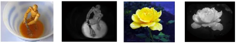
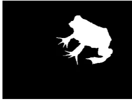
saliency regions from an image via a saliency map. A saliency map is an image with the same size as the input image, in which each pixel value represents its saliency degree. Fig. 1 shows two samples of the saliency map. One can consider that brighter regions in the saliency map represent saliency regions, whereas darker regions indicate the background.
Salient region detection is useful in many applications such as object recognition [2-3], image retargeting [4-5], image quality assessment [6-7], image compression [8-9], and image segmentation [10-11].
Saliency region recognition techniques can be divided into two categories: the bottom-up approach and top-down approach. The bottom-up approach uses low-level features such as color, orientation, and motion, while, the top-down approach, which is task-based driven, uses the high-level features. The values of low-level features at the saliency region have usually unexpected contrast in comparison with the rest of the image. Hence, the rarity of image regions according to its surroundings can be considered for saliency region detection using the low-level feature. Top-down approach uses human vision information to detect salient regions [12] and prior knowledge about the task such as object recognition, and scene classification [1, 13-14].
The existing saliency detection algorithms can be divided into three categories: 1) the methods which only use low-level features, 2) the methods which only use high-level features,
and 3) the methods which use a fusion of low-level and high-level features. In the first approach, the variation of low-level features in different regions of the image is considered for saliency region detection. Indeed, the rarity of image regions according to their surroundings is considered via the calculation of the global or local difference of low-level features. In the local method, the difference in a region is compared with its neighborhoods, while in the global method; the difference in a region is compared with the whole image. Indeed, the rarity of saliency regions produces a bright region in the saliency map which represents the saliency region. It means that a region with more difference compared to other regions of the image will attract more attention of the viewer [12]. Accordingly, there are various patch-based methods in which the input image is initially divided into patches. Then, low- level features are extracted from each patch. Following this, the dissimilarity between image patches is estimated for saliency region detection [15]. Although this approach can partially estimate the saliency region, it suffers from computational complexity.
Top-down approaches usually model human visual experience of detecting salient regions [16], such as location in the image, depth from focus, and supervised learning methods for modeling HVS [17-18].
Generally, current methods of saliency detection suffer from some problems, such as low resolution, non-uniformity, inaccurately defined borders, and computational complexity. Moreover, in top-down approaches, learning high-level features for a computational model is time-consuming and
difficult [12]. Also, modeling an effective fusion model for
combing low-level and high-level features is a challenging task.
In this paper, a new saliency region detection method is proposed which employs both the low-level and high-level features. The proposed method generates uniform salience region and is not time-consuming. In the proposed method, texture difference and color difference in saliency region are considered as low-level features. Wavelet transform and local variance of each channel in Lab color space are utilized to obtain the texture information of the image. Meanwhile, band-pass frequency information of each channel is considered to obtain color information of the image. For high-level features, human’s attention to the center of the image is modeled as a two-dimensional Gaussian function. Finally, the three feature maps are fused to construct the final saliency map. To improve the continuity of the saliency region, some post-processing work is applied on the saliency map.
The rest of the paper is structured as follows: Section 2 reviews related works on saliency region detection. Section 3 describes the proposed approach whereas; Section 4 presents the performance evaluation of the proposed method. Finally, conclusions are drawn in section 5.
2- Related works
There are various works in literature for saliency region detection.
Koch and Ullman in [19] determined salient regions using a
filter named Difference of Gaussians (DoG). A DoG filter is a simple band-pass filter that is able to detect salient regions
[20]. The method in [21] uses an amplitude spectrum of the Fourier transform for saliency region detection. In this method, an input image is divided into non-overlapping patches and the amplitude spectrum of Fourier transform for each patch is calculated as a feature. Finally, saliency regions are detected via using the differences in feature vectors between a patch and all other patches in the image. The resulting saliency map exhibits blurriness and reflects saliency boundaries rather than its entire saliency region.
In [22], Harel et al. proposed the graph-based visual saliency (GBVS) model via using a novel graph-based strategy. This model computes the dissimilarity of center-surround feature histograms. The approach in [16] extracts salient region using a two-directional, two-dimensional PCA on image patches in RGB, YCbCr and Lab color space. Firstly each color channel is divided into non-overlapping patches. Then, two-directional, and two-dimensional PCA are computed on each patch to extract effective features. According to these features, the local and global rarity of each patch is considered for saliency region detection. For local rarity, a contrast model is defined in which a weighted sum of feature differences between a patch and other patches is considered. Finally, saliency maps of each color channel are fused to construct the final saliency map.
In [1], a saliency detection method is proposed via wavelet
transform. At first, the wavelet transform is applied to the input image to create multi-scale feature maps. These maps represent texture and edge information at different scales of the input image. After that, a computational model is proposed for the saliency map via these feature maps. This method extracts accurate boundaries of saliency regions but is incapable of detecting the entire saliency regions.
To reduce the computational complexity, several methods have been proposed to detect saliency regions in the superpixel level rather than in pixel-wise level [15, 23-24]. In [15], firstly, SLIC (simple linear iterative clustering) superpixels [25] are applied on the image to eliminate the unnecessary details. SLIC superpixels segment an image using K-means clustering. After the segmentation process, saliency regions are detected considering the color rarity. In [23], a multi-layer approach is proposed to detect saliency regions. First, three image layers of different scales are obtained from the input image. Then, saliency maps are computed for each layer.
Finally, a saliency map is obtained via fusing them. In [26], an unsupervised multi-scale hierarchical saliency model was proposed, which utilizes both the global and local saliency features. In this approach independent subspace analysis (ISA) is employed, which is equivalent to a two-layer neural architecture.
Recently, high-level features have been utilized for saliency region detection. In [27], similar to HVS, the contextual information to facilitate object searching on natural scenes is explored as a high-level feature. Using Bayesian framework,
this paper proposed an original approach of attentional guidance by the global scene context. In [28], object detection and location are used for salient region detection. In this paper, statistical characteristics of orientation features are utilized as top-down clues to detect the salient regions in natural scenes.
Although low-level and high-level features are useful for saliency region detection per se, employing both of them can further increase the accuracy. In [29], low-level features along with high-level features such as faces, humans, and cars were combined for saliency region detection. In this method, a direct mapping is learned from those features using SVM, regression, and AdaBoost classifiers.
The method in [30] claimed that saliency regions can be detected using three priors. First, the behavior of the human visual system can be modeled by band-pass filtering. Second, the human vision system pays more attention to the center of an image than other regions of the image. Third, cold colors are less attractive to people than the warm ones.
The method proposed in [12] also utilizes both top-down and bottom-up features. Orientation difference and color difference are used to compute bottom-up features. An orientation feature map is computed using local binary patterns (lbp), while color feature map is obtained by
computing color uniqueness and color distribution in Lab color space based on the study [31]. For the top-down feature, depth-from-focus of a single image is used. Salient regions attract the photographer’s attention. Photographers focus on important and attractive objects of the scene (according to their opinion) and other regions are considered out of focus while photographing. Hence, depth-from-focus map estimation is used as a top-down feature. Finally a fusion method is proposed to adjust the weights for different feature maps to construct the final saliency map.
In [32], firstly, a dictionary is learned via patches of natural images. This learned dictionary is used for feature extraction of each patch of the input image. For the salient region detection of an input image, each channel of RGB and HSV color model is divided into non-overlapping patches and
each patch is converted to a vector of coefficients that can
be reconstructed via a learned dictionary. After that, the local and global rarities of each patch are used for salient region detection. The final saliency map is reconstructed via fusing local and global saliency maps of all color channels. This method is time consuming due to the cost of computing local saliency and global saliency for six different color channels. The approach in [33] claims that salient regions are more
aggregative either in texture or color distribution. Firstly, each channel in HSV and Lab color spaces is segmented and the aggregation degree is computed for each segment. Aggregation degree of each segment represents the amount of similarity within a segment. In addition, the amount of diversity between the pixels of different segments is another indicator to detect saliency. After that, the texture saliency map is extracted using the wavelet transform and the Hilber transform. Aggregation degree and divergence are calculated for each segment of texture maps similar to color maps. In the end, the final saliency map is constructed by fusing these feature maps according to the aggregation degree and diversity.
3- Proposed method
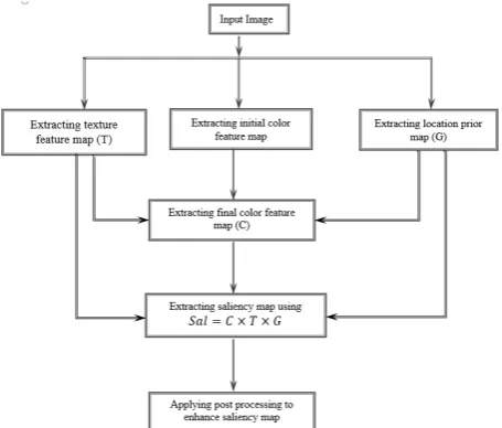
The proposed method in this paper employs color difference, texture difference, and location prior to the detection of saliency region. Fig. 4 exhibits a flowchart of the proposed method. As mentioned before, the image texture features or color features in saliency region are usually unexpected per se [33]; hence, we extract both texture features and color features of the image to detect the saliency region. In addition, different significance of various locations in
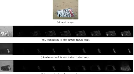
(a) Input image.
(b) L channel and its nine texture feature maps.
(c) a channel and its nine texture feature maps.
(d) b channel and its nine texture feature maps.
Fig. 2. An example of an image and its texture feature maps based on the wavelet from each channel in Lab color space.
(a) Final texture map based on the
is beneficial because of its similarity to human perception and its uniformity [1, 30]. In the following, the proposed method is described in detail.
3- 1- Texture feature map
The proposed texture map integrates two different maps which are obtained using wavelet transform, similar to the method in [1], and local variance in the image. At first, the low-pass Wiener filter is applied to each color channel to remove noise and unnecessary details, then these texture maps are extracted from the denoised image.
The wavelet decomposition can extract the images with low frequencies and high frequencies in the multi-scale perspective. In each decomposition, the LL, LH, HL, and HH sub-bands are created. The LL sub-band indicates the low frequency of the image, while LH, HL, and HH sub-bands represent horizontal, vertical and diagonal details, respectively.
In this paper, nine wavelet decomposition levels are done to create various feature maps at different scales. Each feature map is created by inverse wavelet transform (IWT) of three detailed sub-bands after eliminating LL sub-band at various decomposition levels. Indeed, each feature map contains local variations in multi-scale resolution. In this method, Daubechies mother wavelet with seven samples in length is chosen. Fig. 2 represents nine texture feature maps for each channel in Lab color space. In each row, from left to right, texture feature maps are constructed from the 1st-level (finest scale) to the 9th-level (coarsest scale) wavelet decomposition. The final texture map based on the wavelet is achieved via adding these 27 temporary texture maps. Fig. 3 (a) shows the final texture map using the proposed approach.
To increase the accuracy of the proposed method, in addition to the wavelet texture map, the local variance is also utilized for the tex-ture map. In this method, a sliding window of size (2L+ ×1) (2L+1)
( )
(
)
2(
)
2
, , ,
2 1
L L
k L l L
x i j x i k j l
L =− =−
= + +
+
∑ ∑
(2)where x i j
( )
, is a pixel value at location( )
i j, , x i j( )
,is the local average at the enclosed window, and T2 is the
texture map. In this paper, the size of the window,
(
2L+1)
, is considered 3 experimentally. This feature map is calculated on each channel in Lab color space, hence three texture maps are obtained accordingly. Final texture map based on the local variance is achieved via adding these three temporary texture maps. Fig. 3 (b) shows this texture map. The final texture map is achieved via a weighted combination of these two maps using the following equation:1 1 2 2
T w T w T= × + × , (3)
where T1 and T2 are texture maps based on wavelet and local
variance respectively, w1 and w2 are the associated weights
for these two maps. In this paper, w1 and w2 are considered 3 and 1, respectively to strengthen wavelet based texture map.
3- 2- Color feature map and location prior
Saliency regions may have different colors compared to other regions, hence they attract more attention. It is noteworthy that band frequency is more pronounced to the human visual system than other frequencies. Therefore, band frequency in different channels of Lab color space can be extracted via a band-pass filter. In the proposed method, the Log-Gabor filter, similar to [30], is utilized for the band frequency extraction. Log-Gabor filter in the frequency domain can be formulated as follows [30]:
( )
2 2 20
logu / 2
G u exp σ
ω
= −
, (4)
where u is the coordinate in the R2 frequency domain, 0
ω
is the central frequency of the filter, andσ
controls the filter’s bandwidth.The saliency regions of an image are consistent in one or a few color channels [1]. Fig. 5 shows the band frequency of each channel in Lab color space and the ground-truth. In the first row of this figure, the saliency region is consistent in one channel, whereas, in the second row, none of the channels can represent saliency region separately. Hence, more than one channel is needed to construct the saliency region in the second row. In this paper, all three maps are weighted and combined to construct the final color feature map. To find an appropriate weight for each channel, first an initial estimation for color feature map is considered using the following equation:
2 2 2
1 2 3,
M = C +C +C (5)
the sub-band frequency channels, the following sub-sections should be done.
3- 2- 1- Location prior
Objects near the center of an image attract more attention compared to other regions of the image [30, 34]. Hence, locations near the center of the image are more likely to be saliency regions. This prior can be modeled as a Gaussian function. In this paper, the saliency map of an image using the following function can model the location prior [30]:
2 2 2
x c S exp
σ
−
= −
, (6)
where
x
is the coordinate in the R2 spatial domain,c
andσ
represent the center and the variance of Gaussian function.An example of this map in size 256×256 with the variance of 110 is shown in Fig. 6. It should be mentioned that the center of Gaussian function is considered in the center of the image. In this map, the brighter regions are more likely to be salient regions than the others.
3- 2- 2- Modeling texture saliency map
As mentioned, the saliency map can be obtained using the image texture. This map can be modeled by a Gaussian function. Hence, the center coordinate and variance of Gaussian function should be estimated. First, to estimate the center of Gaussian function, texture feature map is divided into sixteen 64×64 sized regions. From these sixteen regions, four regions are inside and the rest are on the map border. Because of the importance of intermediate regions in the human visual system, one of the four internal regions is considered as a candidate to determine the center coordinate of Gaussian function. To determine the candidate region, the average of each region is calculated. Then, the region with the maximum average value is considered as the best region. Hence, a Gaussian function is considered in center of this region. Fig. 7 shows an example of this process on the texture feature map. In Fig.7(b), the region containing asterisk is the best region, where the center coordinate of Gaussian function is located in the center of this region. Fig. 7(c) represents the estimated Gaussian mapping (with the variance of 110) for saliency regions. Indeed, Fig. 7(c) indicates that saliency regions are towards the top-right of the image.
(a) Original image (b) L channel (c) a channel (d) b channel (e) ground-truth
Fig. 5. Sub-band frequencies of Lab channels.
Fig. 6. Modeling a saliency map based on location prior with a Gaussian function.
(a) Original image (b) Divided saliency texture map into
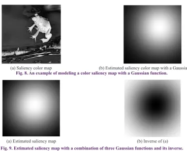
3- 2- 3- Modeling color saliency map
Similarly, the initial color saliency map is modeled with a Gaussian function. Fig. 8 shows an example of this modeling. This estimation, similar to the previous estimation, represents that the saliency regions are towards the top-right of the image.
3- 2- 4- Final color saliency map
By fusing three estimated Gaussian maps, a final estimation of the saliency region can be done using the following equation:
1 2 3
3 2
G = ×G + ×G G+ (7)
where G1, G2, and G3 are the estimated Gaussian maps for saliency regions according to the location, color and texture, respectively. Since saliency regions are usually in the middle of an image, a larger weight is assigned to G1. Also, color is a more prominent feature than texture in our proposed method; hence, a larger weight is intended for color in comparison with the texture.
Fig. 9(a) shows the estimated saliency region according to the above equation in the previous example. It can be observed that saliency region is toward the top-right of the image.
As mentioned, to construct the final color saliency map, a weighted combination of three sub-band frequencies of Lab color channels is needed. The following equations are used to determine the appropriate weights:
(
1 1,
2 2,
3 3)
k
=
S D S
−
−
D S
−
D
, (8)1 1.
S C G= , S2 =C G2. , S3=C G3. , (9)
(
)
1 1. 1
D C= −G , D2 =C2. 1
(
−G)
,(
)
3 3. 1
D C= −G , (10)
where symbol “.” means the inner product, C1, C2, and C3 are sub-band frequencies of each channel in Lab color space, G is estimated Gaussian saliency map and
k
is a triplet which represents the weights for each channel. S1, S2, and3
S represent the similarity of each channel with the estimated Gaussian saliency map, whereas D1, D2, and D3 indicate the dissimilarity of each channel with the inverse of estimated Gaussian saliency map. Indeed, Eq. (8) represents that a high similarity and a low dissimilarity lead to a larger weight in each channel in Lab color space.
It should be mentioned that more similarity between each channel in Lab color space with the estimated Gaussian saliency map, and less dissimilarity between each channel and the inverse of the estimated Gaussian saliency map leads to a larger weight assigned to this channel. Indeed, the low dissimilarity between Lab color channel and the inverse of estimated Gaussian saliency map represents that saliency region is not on the border of the image.
After determining the appropriate weigh for each sub-band color channel, final color saliency map is achieved according to the following equation:
( )
( )
( )
2 2 2
1 1,1 2 1,2 3 1,3
C C= ×k +C ×k +C ×k (11)
3- 3- Saliency region detection via fusing three features In this step, the saliency color map (C ), saliency texture map (T) and Gaussian saliency map (G) are combined to construct the final saliency map. This combination is modeled in the following equation:
Sal C T G
= × ×
(12)As mentioned, to speed up the proposed method, the saliency map is obtained from the down-sampled image. Hence, in this step, the final saliency map is up-sampled to its original resolution. Fig. 10 shows the obtained saliency map in this step.
(a) Saliency color map (b) Estimated saliency color map with a Gaussian function Fig. 8. An example of modeling a color saliency map with a Gaussian function.
(a) Estimated saliency map (b) Inverse of (a)
3- 4- Post-processing
As mentioned before, saliency regions are usually in the center of the image. Accordingly, zero value is assigned to the border of the saliency map with a length of 20 pixels, obtained experimentally, to eliminate unnecessary details. Also, the estimated saliency map with a combination of three Gaussian functions is used to eliminate some unnecessary details. This saliency map is converted into a binary map with a threshold value of 0.25. This value is chosen experimentally. This binary map is multiplied by the saliency map to eliminate some more unnecessary details. In the end, the saliency map is smoothed via applying Wiener filter on it.
Finally, binary saliency map is obtained using an adaptive threshold. The threshold value is determined as twice the average of the saliency map. Fig. 12 shows the results of
the proposed binary saliency map and the ground-truth. As shown in this figure, some of the black pixels were considered white, and some of the white pixels were considered black
erroneously.
A morphological operator can be used to smoothen the image. In this paper, we used an opening operator followed by closing one before the region filling algorithm on the binary saliency map. These operations eliminate narrow joins, small holes, thin gulf, and thin protrusions partly. Fig. 13 (a) shows the effect of morphological operator on the saliency map using the square structuring elements with the size 5×5. Although morphological operator alleviates some noises, some noises remain in the result. Hence, the connected components technique is utilized for further improvement. In the binary map, the neighboring pixel with the same value is constituted as a connected component. Eight neighbors of a pixel are considered to determine a neighboring pixel. Hence, all of the pixels in the saliency map are located in some components. Some of these components are noise. To identify noise components, the existing pixels in each component are counted. Components containing a few pixels are considered as noise, hence eliminated. We considered the threshold value dependent on the image size, 1/45 of the total number of pixels in the image. Fig. 13 (b) shows the effect of connected components technique.
Fig. 10. An example of our proposed final saliency map.
(a) Binary Gaussian saliency map. (b) Post-processed saliency map. Fig. 11. Results of post-processing of saliency map.
(a) The proposed binary saliency map. (b) Ground-truth.
Fig. 12. Results of the proposed binary saliency map and the ground-truth.
4- Experimental results
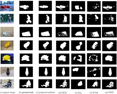
In this paper, MSRA database is used to evaluate the proposed method with several state-of-art methods. MSRA database contains 1000 color images and their corresponding ground-truth. The proposed method is compared with four well-known methods: FBTF1 [12], WTM2 [1], ISA [26], and
SDSP3 [30] both subjectively and objectively. Fig. 14 shows
some samples of this comparison. The results show that the proposed binary saliency map is uniform and also more similar to the ground-truth than the other compared methods.
4- 1- Performance measurement
Objective assessment is considered to compare the similarity between the binary saliency maps and the ground-truths.
Precision, Recall, and F-Measure are defined according to the following formulas [1]:
(
) (
)
(
)
(
)
1 1
1 1
, ,
,
M N
x y
M N
x y
t x y s x y
Precision
s x y
= =
= =
×
=
∑ ∑
∑ ∑
(13)1 Fusing Bottom-Up and Top-Down Features 2 Wavelet Transform Method
3 Saliency Detection by Combining Simple Priors
(
) (
)
(
)
(
)
1 1
1 1
, ,
,
M N
x y
M N
x y
t x y s x y
Recall
t x y
= =
= =
×
=
∑ ∑
∑ ∑
(14)(
1)
P RF measure
P R
α α
+ × ×
− =
× + (15)
where, s x y
(
,)
represents the pixel of binary saliency map in positions(
x y,)
, t x y(
,)
demonstrates the corresponding pixel in the ground-truth, andα
is a non-negative parameter determining the importance of the precision over the recall.α
is set 0.3 to weight precision rate more than recall rate [24, 28]. The average precision, recall, and F-measure values of the proposed method and the four compared methods on 1000 images from MSRA database are illustrated in Fig. 15. It can be seen the proposed method produces better objective values than the other four algorithms. Of course, the recall value of the FBTF method is slightly larger than the proposed method, while precision and F-measure values of the proposed method are larger than those of the FBTF method.4- 2- Comparing Running Time
The average consuming time for saliency region detection of the proposed method and the four existing methods on MSRA database are shown in Table 1. All the algorithms
were implemented in Matlab and run on a computer with a 2.40 GHz Intel Corei7 and 8G of RAM. It can be seen that the methods introduced in [26, 30] are faster than the proposed method. But based on subjective and objective comparison, the proposed saliency region detection is more accurate than the ones reported in [26, 30].
5- Conclusions
In this paper, we have proposed a new method for saliency region detection. The proposed method utilizes both low-level and high-low-level features. Although the low-low-level and high-level features are useful for saliency region detection per se, employing both can improve the accuracy further. Also, at the post-processing step, morphological operator and connected components technique are used to smooth the saliency map and remove noises. The results showed that the proposed method outperforms the existing saliency region detection methods in terms of objective and visual quality. References
[1] N. Imamoglu, W. Lin, Y. Fang, A saliency detection model using low-level features based on wavelet transform,
IEEE transactions on multimedia, 15(1) (2012) 96-105. [2] J. Zhang, S. Sclaroff, Z. Lin, X. Shen, B. Price, R. Mech,
Unconstrained salient object detection via proposal subset optimization, in: Proceedings of the IEEE conference on computer vision and pattern recognition, (2016) 5733-5742.
[3] D. Walther, C. Koch, Modeling attention to salient proto-objects, Neural networks, 19(9) (2006) 1395-1407. [4] C.-C. Hsu, C.-W. Lin, Y. Fang, W. Lin, Objective quality
assessment for image retargeting based on perceptual
geometric distortion and information loss, IEEE Journal of Selected Topics in Signal Processing, 8(3) (2014) 377-389.
[5] S. Avidan, A. Shamir, Seam carving for content-aware image resizing, in: ACM Transactions on graphics (TOG), ACM (2007) 10.
[6] L. Zhang, Y. Shen, H. Li, VSI: A visual saliency-induced index for perceptual image quality assessment, IEEE Transactions on Image Processing, 23(10) (2014) 4270-4281.
[7] W. Zhang, A. Borji, Z. Wang, P. Le Callet, H. Liu, The application of visual saliency models in objective image quality assessment: A statistical evaluation, IEEE transactions on neural networks and learning systems, 27(6) (2015) 1266-1278.
[8] C. Guo, L. Zhang, A novel multiresolution spatiotemporal saliency detection model and its applications in image and video compression, IEEE transactions on image processing, 19(1) (2009) 185-198.
[9] X.Y. Stella, D.A. Lisin, Image compression based on visual saliency at individual scales, in: International Symposium on Visual Computing, Springer (2009) 157-166.
[10] Z. Li, G. Liu, D. Zhang, Y. Xu, Robust single-object image segmentation based on salient transition region,
Pattern recognition, 52 (2016) 317-331.
[11] W. Zou, Z. Liu, K. Kpalma, J. Ronsin, Y. Zhao, N. Komodakis, Unsupervised joint salient region detection and object segmentation, IEEE Transactions on Image Processing, 24(11) (2015) 3858-3873.
[12] H. Tian, Y. Fang, Y. Zhao, W. Lin, R. Ni, Z. Zhu, Salient region detection by fusing bottom-up and top-down features extracted from a single image, IEEE Transactions on Image processing, 23(10) (2014) 4389-4398.
[13] S. Frintrop, VOCUS: A visual attention system for object detection and goal-directed search, Springer, 2006. [14] L. Itti, Models of bottom-up and top-down visual
attention, California Institute of Technology, 2000. [15] F. Perazzi, P. Krähenbühl, Y. Pritch, A. Hornung,
Saliency filters: Contrast based filtering for salient region detection, in: 2012 IEEE conference on computer vision and pattern recognition, IEEE, (2012) 733-740.
[16] Y.-Y. Zhang, X.-Y. Liu, H.-J. Wang, Saliency detection via two-directional 2DPCA analysis of image patches,
Optik-International Journal for Light and Electron Optics, 125(24) (2014) 7222-7226.
[17] J.M. Wolfe, T.S. Horowitz, What attributes guide the deployment of visual attention and how do they do it,
Nature reviews neuroscience, 5(6) (2004) 495.
[18] B. Rasolzadeh, A.T. Targhi, J.-O. Eklundh, An Fig. 15. Objective comparison of four different methods with
our proposed method.
Table 1. The average computational time, in seconds per image, for the methods introduced in [1, 12, 26, 30] and the proposed method.
Proposed method FBTF
ISA SDSP
WTM
4.5910 [sec/image] 19.5130 [sec/image]
3.1480 [sec/image] 0.5333 [sec/image]
[20] R. Achanta, S. Hemami, F. Estrada, S. Süsstrunk, Frequency-tuned salient region detection, in: IEEE
International Conference on Computer Vision and Pattern Recognition (CVPR) (2009) 1597-1604.
[21] Y. Fang, W. Lin, B.-S. Lee, T. Lau, Z. Chen, C.-W. Lin, Bottom-up saliency detection model based on human visual sensitivity and amplitude spectrum, IEEE Transactions on Multimedia, 14(1) (2011) -187-198. [22] J. Harel, C. Koch, P. Perona, Graph-based visual
saliency, in: Advances in neural information processing systems, (2007) 545-552.
[23] Q. Yan, L. Xu, J. Shi, J. Jia, Hierarchical saliency detection, in: Proceedings of the IEEE Conference on
Computer Vision and Pattern Recognition, 2013, pp.
1155-1162.
[24] W. Zhu, S. Liang, Y. Wei, J. Sun, Saliency optimization from robust background detection, in: Proceedings of the IEEE conference on computer vision and pattern recognition, 2014, pp. 2814-2821.
[25] R. Achanta, A. Shaji, K. Smith, A. Lucchi, P. Fua, S. Süsstrunk, Slic superpixels, 2010.
[26] H.R. Tavakoli, J. Laaksonen, Bottom-up fixation prediction using unsupervised hierarchical models, in:
Asian Conference on Computer Vision, Springer, 2016, pp. 287-302.
for salient object detection, in: 2011 IEEE International Conference on Acoustics, Speech and Signal Processing (ICASSP), IEEE, 2011, pp. 1293-1296.
[29] A. Borji, Boosting bottom-up and top-down visual features for saliency estimation, in: 2012 IEEE
Conference on Computer Vision and Pattern Recognition, IEEE, 2012, pp. 438-445.
[30] L. Zhang, Z. Gu, H. Li, SDSP: A novel saliency detection method by combining simple priors, in: 2013
IEEE international conference on image processing, IEEE, 2013, pp. 171-175.
[31] F. Perazzi, P. Krähenbühl, Y. Pritch, A. Hornung, Saliency filters: Contrast based filtering for salient region detection, in: 2012 IEEE conference on computer vision and pattern recognition (CVPR), IEEE, 2012, pp. 733-740.
[32] A. Borji, L. Itti, Exploiting local and global patch rarities for saliency detection, in: 2012 IEEE conference on computer vision and pattern recognition, IEEE, 2012 pp. 478-485.
[33] Y. Wo, X. Chen, G. Han, A saliency detection model using aggregation degree of color and texture, Signal Processing: Image Communication, 30 (2015) 121-136. [34] T. Judd, Learning to predict where humans look IEEE
international conference on computer vision, Proc. ICCV, 2009. (2009)
Pleasecitethisarticleusing:
S. Asadi Amiri, H. Hassanpour, A Saliency Detection Model via Fusing Extracted Low-Level and High-Level Features
from an Image, AUT J. Elec. Eng., 51(1) (2019) 3-12.

![Table 1. The average computational time, in seconds per image, for the methodsintroduced in [1, 12, 26, 30] and the proposed method.](https://thumb-us.123doks.com/thumbv2/123dok_us/14642.2001404/9.595.42.278.230.428/table-average-computational-seconds-image-methodsintroduced-proposed-method.webp)
