AUT J. Civil Eng., 2(1) (2018) 39-48 DOI: 10.22060/ajce.2018.14511.5480
Performance Assessment of Grasshopper Optimization Algorithm for Optimizing
Coefficients of Sediment Rating Curve
M.J. Zeynali*, A.Shahidi
Department of Water Engineering College of Agriculture University of Birjand, Birjand, Iran
ABSTRACT: One of the most common methods for estimating suspended sediment of rivers is sediment rating curve. For better estimation of the amount of suspended sediment based on the sediment curve rating equation, it is possible to optimize its coefficients. One of the methods used for optimizing the coefficients of the sediment curve rating equation is taking advantage of meta-heuristic algorithms. The main objective of this research is the use of grasshopper optimisation algorithm to optimize the relationship between discharge and sediment discharge and comparison the results of this model with genetic algorithms and particle swarm. With respect to the objective function, which minimizes the difference between the measured values of the sediment and the calculated values of that, the optimal values of these coefficients are determined. The results of this research indicated since the objective function, grasshopper optimisation algorithm compared with Genetic algorithm and particle swarm optimization has a good performance. So that grasshopper optimisation algorithm with 7694507 values has the best performance in this problem and then PSO and GA algorithms with 7702357 and 7703750 have a good performance and finally this value in sediment rating curve is equal to 9163544.
Review History:
Received: 28 March 2018 Revised: 21 April 2018 Accepted: 23 April 2018 Available Online: 1 July 2018
Keywords: Genetic Algorithm
Met-Heuristic Algorithm Particle Swarm Algorithm Suspended Sediment
1- Introduction
Correct estimation of the concentration of sediment in rivers is of great importance for planning and managing water resources projects. The sediment rating curve can be considered as one of the most common methods for estimating suspended sediment. One of the methods for better estimating the suspended sediment content based on the equation of the sediment rating curve, is to optimize the coefficients of this equation. The optimization of the sediment rating curve coefficients and the measurement of the discharge rate that is easier than measurement of sediment, provides more accurate and more realistic estimate of suspended sediment. The evaluation of flow discharge and suspended sediment discharge relationships and optimization of the coefficients of the sediment rating curve equation have been considered both in Iran and abroad; and engineers, have used the meta-heuristic algorithms, which is one of the methods for optimizing the coefficients of the sediment rating curve equation.
Altunkaynak has estimated the amount of sediment using the discharge values through the genetic algorithm [1].
Mohammad Reza Pour et al. used a genetic algorithm to optimize the relationship between flow discharge rate and sediment discharge for Nodeh station located on Gorganrood River that, the results were compared with the sediment rating curve. The evaluation of the results showed that the genetic algorithm has a higher accuracy than the sediment rating curve [2]. Ebrahimi et al. investigated the performance of bee algorithm in suspended sediment content and concluded that the bee algorithm has a high efficiency [3]. Mohammad Reza Pour and Zeynali in a study compared the ant colony algorithm and elitist ant algorithm and Max-min ant algorithm in optimizing sediment rating curve coefficients and the results showed that according to the root mean square error (RMSE) and Nash-Sutcliff coefficient (NC), the elitist ant algorithm with RMSE was 32738.54 and Nash coefficient is 0.440, and then the ant colony algorithm with values of 33479.00 and 0.415, and then the max-min ant algorithm with the value of 34552.77 and 0.376 respectively had the best performance. Finally, the sediment rating curve has had the values of 35305.53 and 0.349 for root mean square error and Nash-Sutcliff coefficient [4]. Talebi et al., in a study determined the optimized sediment equation and its relationship with the physical characteristics of the basin in semi-arid regions and concluded that the mean slope of the
basin has a direct relationship with the coefficient b in the rating curve equation and the optimized equation can be used to predict the sediment content on an annual scale [5]. The meta-heuristic algorithms in optimization should have two important phases of “exploration” and “exploitation”. The search means that members of the population in an algorithm must be able to search the entire space for possible solutions, and exploitation means that, population members must be able to search around an optimal solution. For example, the operation of the mutation in the genetic algorithm performs the search phase, and the crossover operation performs the exploitation phase but only a few populations (given the percentage of mutations) do this but in the Grasshopper
optimization algorithm, all grasshoppers perform this
exploration, therefore, the probability of finding the best optimal solutions in the search phase will be greater and in
this perspective, the Grasshopper optimization algorithm has
a different function than other algorithms and this difference is also considered as an advantage.
The main objective of this study was to evaluate the efficiency of grasshopper optimization algorithm in optimizing sediment rating curve equation coefficients and compare it with particle swarm algorithm and genetics and finally compare the results obtained from these algorithms with the sediment rating curve equation. Therefore, the performance of each algorithm will be analyzed and evaluated according to the objective function after introducing the algorithms and examining the structure, their characteristics and parameters.
2- Materials and methods
2- 1- Case study
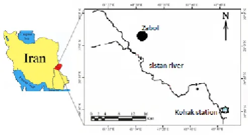
The Helmand River originates from the southern slopes of the Hindu Kush Mountains near Kabul and after passing about 1000 kilometers reaches the Iranian border. This river is divided into two common branches of Parian and the Sistan River on the border between Iran and Afghanistan. Sistan River is the most important water source in Sistan plain, which passes about 70 km from Sistan plain to Hamoun Helmand. This river with a general slope of 0.00002-0.00006 from a level of 489 meters in two branches of Helmand reaches the level of 474.75 meters in Hamoun Helmand. The time series under study is the flow discharge rate data (m3/s) and the sediment load data (ton/day) of the Kohak station. This station is located along the geographical longtitude of 45° 61’ and latitude 49° 30’ north. [6]. Figure 1 shows the location of the Kohak station in Sistan and Baluchestan province and Table 1 shows the hydrometric conditions and the statistical characteristics of the data in the statistical period for the Sistan River. The statistical period considered in this research is from 1970 to 2010.
Table 1. The statistical parameters of Sistan River in studied time period
flow discharge (m3/s) suspended sediment (ton/day)
average maximum minimum average maximum minimum
66.09 599.00 0.20 25028.52 411220.80 1.33
2- 2- Objective Function
The purpose of this research is to minimize the difference between the measured sediment content (actual sediment)
Q0 and the calculated sediment values Qm using the proposed models whose function has been defined in the form of Equation 1. In this function, the unit of Q0 and Qm is both in terms of tons per day.
Figure 1. Geographic Location of Studied Area
(1)
2
1
( ) l ( m o)
i
g u Q Q
=
=
∑
−In the above equation, u is the input factor and g (u) is the objective function that must be minimized. Since the calculated sediment content is a function of parameters such as daily discharge of the river Qw, to minimize the objective
function it is necessary to look for parameters which approach
Qm to Q0.
In this study, the relation between sediment discharge and flow discharge is defined as Equation 2 [7, 8]:
(2) b
m w
Q
=
aQ
Where Qw is daily flow discharge (cubic meters per second);
(a) and (b) are non-dimensional coefficients that should be optimized. According to the study area and the data studied in this paper, the upper and lower limits for coefficients (a) and (b) were considered as 0.001 and 200, 0.001 and 3
respectively.
2- 3- Performance Criteria
Performance of each algorithm calculated by mean absolute error (MAE) criteria end the other criteria like mean square error (MSE), root mean square error (RMSE), sum square error (SSE), Nash-Sutcliffe coefficient and correlation. These performance criteria calculated by Equations 3 to 8. Where
Qi is observation values is calculated values n is number of data.
ˆi
(3) 1 ˆ | | n i i i Q Q MAE n = − =
∑
(4) 2 11 n ( ˆ)
i i
i
MSE Q Q
n = =
∑
− (5) 0.5 2 11 n ( ˆ)
i i
i
RMSE n Q Q
= = −
∑
(6) (7) 2 1 2 1 ˆ ( ) 1 ( ) n i i i n i i i Q Q NS Q Q = = − = − −∑
∑
1 1 1
2 2 2 2
1 1 1 1
ˆ ˆ
( )( ) ( )( )
ˆ ˆ
( ) ( ) ( ) ( )
n n n
i i i i
i i i
n n n n
i i i i
i i i i
n Q Q Q Q
R
n Q Q n Q Q
= = = = = = = − = − −
∑
∑ ∑
∑
∑
∑
∑
(8)2- 4- Grasshopper Optimization Algorithm (GOA)
Grasshopper are insects. They are considered a pest due to their damage to crop production and agriculture. Although grasshoppers are usually seen individually in nature, they join in one of the largest swarm of all creatures. The size of the swarm may be of continental scale and a nightmare for farmers. The unique aspect of the grasshopper swarm is that the swarming behavior is found in both nymph and adulthood. Millions of nymph grasshopper jump and move like rolling cylinders. In their path, they eat almost all vegetation. After this behavior, when they become adult, they form a swarm in the air. This is how grasshoppers migrate over large distances. The main characteristic of the swarm in the larval phase is slow movement and small steps of the grasshoppers. In contrast, long range and abrupt movement is the essential feature of the swarm in adulthood. Food source seeking is another important characteristic of the swarming of grasshoppers. Nature inspired algorithms logically divide the search process into two tendencies: exploration and exploitation. In exploration, the search agents are encouraged to move abruptly, while they tend to move locally during exploitation. These two functions, as well as target seeking, are performed by grasshoppers naturally. The mathematical model employed to simulate the swarming behavior of grasshoppers is presented as follows [9].
i i i i
X = +S G A+ (9)
Where Xi defines the position of the i-th grasshopper, Si
is the social interaction, Gi is the gravity force on the i-th grasshopper, and Ai shows the wind advection. Note that to provide random behaviour the Equation 9 can be written as Equation 10.
1 2 3
i i i i
X =r S r G r A+ + (10)
Where r1 , r2 , and r3 are random numbers in [0,1]. Social interaction (Si) in Equation 9 can be calculated as Equation
11.
( )
1
ˆ
n
i ij ij
j j i
S
s d d
=
=
∑
(11)where dij is the distance between the i-th and the j-th grasshopper, calculated as , s is a function to define the strength of social forces, as shown in Equation 12, and is a unit vector from the i-th grasshopper to the j-th grasshopper [10].
ij j i
d = X −X
ˆ j i ij ij X X d d − = (12)
( ) lr r
s r = fe− −e−
Where f indicates the intensity of attraction and l is the attractive length scale. For choose the value of f the interval can be between zero and one and for l between one and two. But in general, the recommended values for f and l are respectively 0.5 and 1.5 [10]. The G and A component in Equation 9 can be calculated as Equations 13 and 14.
(13) ˆ
i g
G = −g e
(14) ˆ
i w
A u e=
Where g is the gravitational constant and shows a unity vector towards the centre of earth. u is a constant drift and is a unity vector in the direction of wind. Substituting S, G, and A in Equation 9, this equation can be expanded as follows:
ˆg e ˆw e (15)
(
)
1 ˆ ˆ n j ii j i g w
j ij
j i
X X
X s X X g e u e
d =
≠
−
=
∑
− − +This mathematical model cannot be used directly to solve optimization problems, mainly because the grasshoppers quickly reach the comfort zone and the swarm does not converge to a specified point. A modified version of this equation is pro- posed as follows to solve optimization problems [10]: (16)
(
)
1 ˆ 2 n j id d d d d
i j i d
j ij
j i
X X ub lb
X c c s X X T d = ≠ − − = − +
∑
Where ubd is the upper bound in Dth dimension, lbd is the
lower bound in the Dth dimension equation. is the value of the Dth best solution found so far, and c is a decreasing coefficient to shrink the comfort zone, repulsion zone, and attraction zone. Also, we do not consider gravity (G component) in Equation 16 and assume that the wind direction (A component) is always towards a target ( ) [10].
( ) lr r
s r =fe− −e− ˆ
d
T
ˆd
T
max min
max
c
c
c c
l
L
−
=
−
(17)Where cmax is the maximum value, cmin is the minimum value, l indicates the current iteration, and L is the maximum number of iterations. In this work, we use 1 and 0.00001 for
cmax and cmin respectively.
2- 5- Genetic Algorithm
The genetic algorithm is an optimization technique inspired by live nature which can be categorized as a numerical, direct and random search method. This algorithm is based on repetition, and its principles have been adapted from genetics. 2 1 ˆ ( ) n i i i
SSE Q Q
=
There is the main (primary) population in the genetic algorithm from which the population is generated by the crossover operation (children) and the population is mutated that, the two populations are merged with the initial population and finally, they will be extracted according to the performance of population members and the value of the objective function as much as the initial population. In general, the cycle of the genetic algorithm is such that initially a primary population of individuals is selected, regardless of the specific criteria and randomly. For all zero-gen chromosomes (subjects), the fitness is determined according to the objective function; then, a subset of the primary population will be selected with the different mechanisms defined for the selection operator. Then, cutting and mutation operations will be selected, if necessary on these selected individuals, depending on the problem. Now, those people to whom the mechanism of genetic algorithms is applied, should be compared with the initial population (zero generation) in terms of fitness. However, people with the highest fitness will remain. Such individuals will act as the initial population for the next step of the algorithm. Each iteration step of the algorithm generates a new generation, which will evolve, according to the modifications made. Here it should be noted that the algorithm can be used in different ways to codify decision variables, parent selection, type of chromosome combination, how to mutate, etc that, some of the methods are introduced in the following [11]:
The coding methods are: coding as direct, indirect, mutation, value, tree coding. Parent selection methods for crossover operation are: Selection by roulette wheel, competitive selection, sequential selection, steady state, Boltzmann’s method, elitism, cutoff, Brindle and race. Methods of crossover are: single-point, two points, uniform displacement multi-points, sequential, cycles and convex crossover. The methods for performing mutation operations are: reversing the bit, changing the ordering, reversing, and changing the value.
2- 6- Particle Swarm Optimization
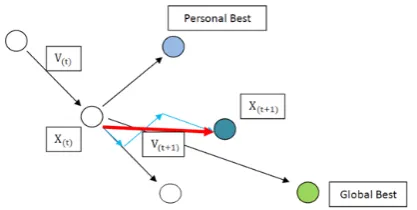
The particle swarm algorithm is also known as another names such as algorithm of birds; like other meta-heuristic algorithms, it creates a random population of individuals. The basis of the algorithm is that, any action and reaction affect the group movement and subsequently, each member of the set can enjoy the discoveries and skills of other members of the group. The difference between the particle swarm algorithm and other evolutionary algorithms is in the way through which the population created moves in the search space. As,
Figure 2. Comfort zone and attraction and repulsion force in this area
at any given moment, each component set its position in the
search space, according to the best place ever posited and the best location that found in the entire group (population). It can be said that the movement of the group is the result of the efforts of all members. The movement and displacement of a component (particle) is such that when a particle with a
velocity vector V(t) arrives a new position from the previous location in space, at this position, it can go with the velocity vector to the best position ever to be there (Personal Best) or, goes with the velocity vector to the best position ever found by the whole group (Global Best) or continuing its path in the same direction; in this case, none of the choices alone is appropriate and the particle should select and move with the combination of the above-mentioned directions. Therefore, the new velocity vector V(t+1) is calculated according to Equation 18 [11]:
(18)
(
)
(
)
( 1)t . ( )t 1 1. . ( )t ( )t 2 2. . ( )t ( )t
V + =w V +C r P −X +C r G −X
Where C1 and C2 are constant numbers; r1 and r2 are random vectors between zero and one; P(t) is the best position where the particle X has ever had and G(t) is the position of the best place where all the particles have been found so far. The new position is also calculated according to Equation 19:
(19)
( 1)t ( )t ( 1)t
X + =X +V+
Where, X(t) is the previous position and X(t+1) is the current position of the particle. Figure 3 shows the above mentioned cases [11].
Figure 3. Moving particle from point to point in the particle swarm optimization
3- Results
In each algorithm, various scenarios can be studied by changing parameters and methods. For example, in the genetic algorithm, as described in the material and methods, different methods can be used in the coding method to select how parents choose for crossover, and mutate operations. In this research, value coding method, parent selection using roulette wheel, single point, two point and multipoint crossover, and mutation operation have been done by changing the value. Other parameters of this algorithm and particle swarm algorithm are also given in Table 2.
The parameters of the grasshopper optimization algorithm
are also examined by the trial and error, and the most suitable values for the parameters of this algorithm are given in Table
Table 2. Parameters that used in GA and PSO algorithms
genetic algorithm particle swarm optimization
number of iteration 400 number of iteration 400
number of population 50 number of population 50
number of Parents 40 C1 parameter 1.5
Number of parents per total population 0.8 C2 parameter 2.5
Number of mutants per total population 0.4 max and min of velocity in 1st dimension
(a in ) 0.005 of number of iteration
Probability of single point crossover 1 max and min of velocity in 2th dimension
(b in ) 0.005 of number of iteration Probability of double point crossover 0 gradient weighted (w) 0.6
Probability of multipoint crossover 0 … 0.99
b
m w
Q =aQ
b
m w
Q =aQ
Table 3. The best values of parameters for grasshopper optimization algorithm
number of iteration number of population attractive length
scale (l) intensity of attraction (f) Cmax parameter Cmin parameter
400 50 0.75 1.0 1.0 0.00001
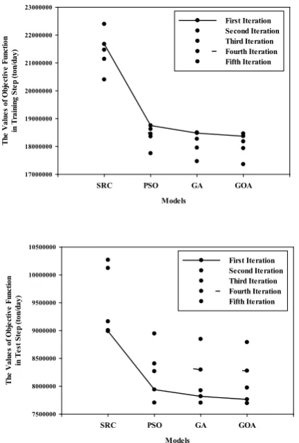
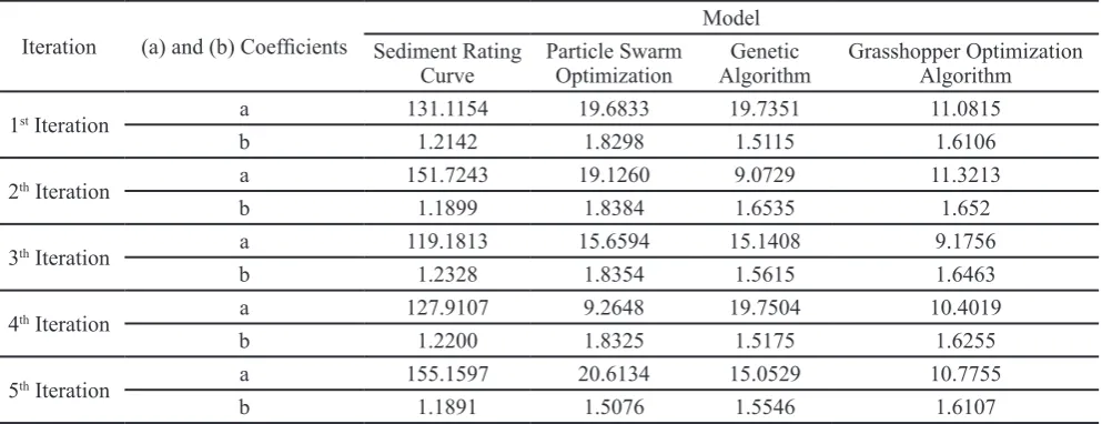
After models were trained with 70% of randomly selected data, the models were tested with 30% of the rest of the data. When one of the algorithms divides the data randomly into two classes of training and testing, the same data is used for other algorithms so the conditions for all algorithms are identical. Regarding this, based on the value of the objective function, the results showed that the algorithms had the most appropriate performance in the fifth iteration, and in this iteration, the grasshopper optimization algorithm with the value of the objective function of 7694507 has the best performance in this problem and then the GA and PSO algorithms with the values of 7702357 and 7703750 had the best performance. Finally, this value in the sediment rating curve is 9163544. The summary of the results of each of the five iterations is also presented in Table 4 and Figure 4. According to Table 4 and Figure 4, the grasshopper optimization algorithm has a better performance than other algorithms and sediment rating curve in all replications. Of course, except for one case in the test section, in the third repetition, the performance of the genetic algorithm was better than the grasshopper optimization algorithm. But in general, it can be said that in the problem of optimizing the coefficients of the sediment rating curve equation, all algorithms have higher efficiency than sediment rating curve equation in estimation of suspended sediment content due to finding more appropriate values for these coefficients and among the algorithms examined, according to the values of the objective function, the efficiency of the GOA algorithm is greater than other algorithms. Also, the optimal values of the coefficients (a) and (b), which are optimized by each of the algorithms, along with the coefficients of the sediment rating curve equation are presented in Table 5.
Figure 4. Performance of algorithms in each iteration for train and test
Models
SRC PSO GA GOA
The
V
al
ue
s
of
O
bj
ec
tiv
e
Func
tio
n
in
Tr
ai
ni
ng
S
te
p
(to
n/
da
y)
17000000 18000000 19000000 20000000 21000000 22000000 23000000
First Iteration Second Iteration Third Iteration Fourth Iteration Fifth Iteration
Models
SRC PSO GA GOA
The
V
al
ue
s
of
O
bj
ec
tiv
e
Func
tio
n
in
Te
st
S
te
p
(to
n/
da
y)
7500000 8000000 8500000 9000000 9500000 10000000 10500000
Other criteria have been investigated to investigate the performance of algorithms where the results for all repetitions are roughly the same and provide the same pattern of algorithm performance. Therefore, the results of the fifth repetition are given in Table 6 as examples.
As shown in Table 6, considering the objective function, GOA algorithm has a better performance than the GA and PSO algorithms. But according to the SSE, MSE, RMSE, (R) and Nash-Sutcliff (NS) Correlation criteria, the results showed an inappropriate performance of the algorithms and, as the algorithm performs better in terms of the objective function, it has had an inappropriate performance in terms of other criteria. But according to the MAE criterion, the GOA algorithm also has a better performance than other algorithms. Because this criterion is very similar to the objective function. However, since the algorithms seek to minimize the objective
Table 4. The Value of Objective Function in Each Iteration for All Models (ton/day)
Objective Function Part Sediment Rating Model
Curve Particle Swarm Optimization Genetic Algorithm Grasshopper Optimization Algorithm
1st Iteration Train 21675040 18750533 18479061 18367390
Test 8989073 7938862 7818124 7763081
2th Iteration Train 21140497 18357734 17950699 17934468
Test 10122086 8402546 8296497 8276785
3th Iteration Train 21467936 18449369 18267357 18178606
Test 9005498 8267926 7923870 7973119
4th Iteration Train 20402864 17750289 174677078 17358480
Test 10268308 8945457 8847158 8790018
5th Iteration Train 22394196 18623701 18495738 18461044
Test 9163544 7703750 7702357 7694507
Table 5. The value of (a) and (b) coefficients in each iteration for all models
Iteration (a) and (b) Coefficients Sediment Rating Model
Curve Particle Swarm Optimization AlgorithmGenetic Grasshopper Optimization Algorithm
1st Iteration a 131.1154 19.6833 19.7351 11.0815
b 1.2142 1.8298 1.5115 1.6106
2th Iteration a 151.7243 19.1260 9.0729 11.3213
b 1.1899 1.8384 1.6535 1.652
3th Iteration a 119.1813 15.6594 15.1408 9.1756
b 1.2328 1.8354 1.5615 1.6463
4th Iteration a 127.9107 9.2648 19.7504 10.4019
b 1.2200 1.8325 1.5175 1.6255
5th Iteration a 155.1597 20.6134 15.0529 10.7755
b 1.1891 1.5076 1.5546 1.6107
Table 6. The value of performance criteria of algorithms in test of 5th iteration
Algorithms Objective Function (ton/day)
Performance Criteria
SSE (ton/day) (ton/day)MSE (ton/day)RMSE (ton/day)MAE R NS
Particle Swarm Optimization 7703750 6.04951×10¹¹ 939364441.5 30649.05 11962.34 0.8732 0.7571
Genetic Algorithm 7702357 6.25914×10¹¹ 971916561.5 31175.58 11960.18 0.8709 0.7486
Grasshopper Optimization
Algorithm 7694507 6.38608×10¹¹ 991627263.7 31490.11 11947.99 0.8679 0.7435
Table 7. The value of performance criteria of algorithms in test of 5th iteration
Models Objective Function
(MSE) (ton/day) SSE Performance Criteria in Test
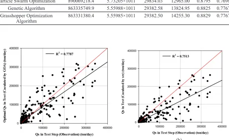
(ton/day) (ton/day)RMSE (ton/day)MAE R NS Sediment Rating Curve 1194957550.4 7.69553×10¹¹ 34568.16 12797.54 0.8668 0.690955
Particle Swarm Optimization 890069218.4 5.73205×10¹¹ 29834.03 12965.00 0.8795 0.769806
Genetic Algorithm 863335749.9 5.55988×10¹¹ 29382.58 13824.95 0.8825 0.776720
Grasshopper Optimization
Algorithm 863331380.4 5.55985×10¹¹ 29382.50 14255.30 0.8829 0.776721
Qs in Test Step (Observation) (ton/day)
0 100000 200000 300000 400000
O
pt
im
al
Q
s
in
Te
st
(C
ac
ul
at
ed
by
G
O
A
) (
to
n/
da
y)
0 100000 200000 300000 400000
R2 = 0.7787
Qs in Test Step (Observation) (ton/day)
0 100000 200000 300000 400000
Q
s
in
Te
st
(C
ac
ul
at
ed
by
s
rc
) (
to
n/
da
y)
0 100000 200000 300000 400000
R2 = 0.7513
Figure 5. Comparison observed and calculated of suspended sediment by GOA (a) and SRC (b) model(a)
(b)
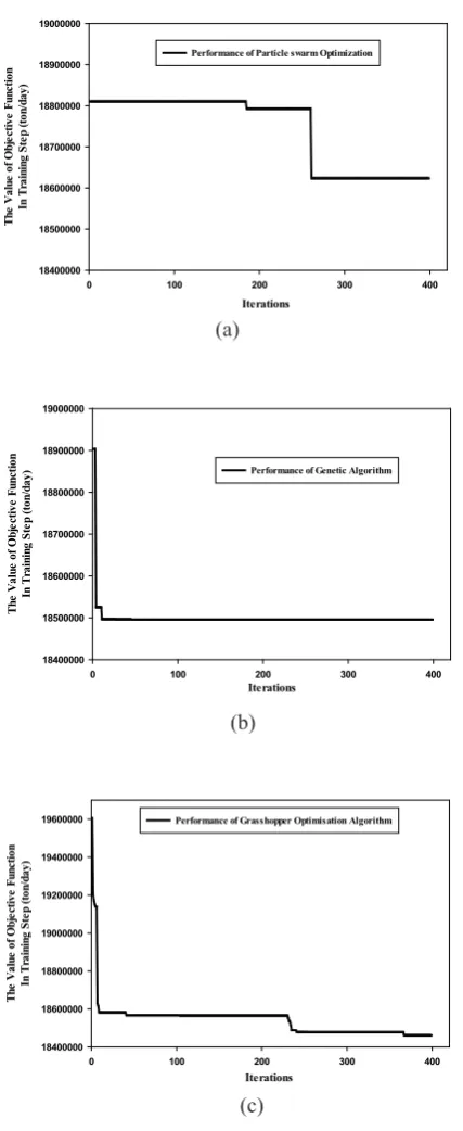
In the following, the graph of changes in the objective function versus iteration for the training section of the algorithms of each of the PSO, GA and GOA algorithms has been presented in Figures 6a to 6c, respectively.
Also, along with the results, the average time elapsed for each algorithm to reach the maximum number of replicates (400 repetitions) is calculated and the results have been presented in Table 8 and as seen in this table, the elapsed
time to reach 400 repetitions for all three algorithms is less
than two minutes and in the meantime, the particle swarm
4- Discussion and Conclusion
The purpose of this research was to evaluate the efficiency
of grasshopper optimization algorithm in optimizing
sediment rating curve coefficients in suspended sediment estimation. In this regard, 40-year-old flow discharge data and sediment discharge measured at the Kohak station on the Sistan River in southeastern Iran were used. After testing models with 70% of the data, they were tested with 30% of the data and the results showed that, considering the objective function of the grasshopper optimization algorithm, it has higher efficiency than the two genetic and particle swarm algorithms. Therefore, the grasshopper optimization algorithm with the value of the objective function 7694507 has the best performance in this problem and then the GA and PSO algorithms with the values of 7702357 and 7703750 had the highest performance. Finally, this value is 9163544 in the sediment rating curve. The high efficiency of the GOA algorithm can be found in the specific features of this algorithm. In general, an appropriate algorithm must also be able to search the entire space for solutions and it can search around an optimal possible solution. In the GA algorithm, the exploration section performs the mutation phase and the exploitation part (local search) performs the crossover phase. But considering the percentage of mutation, only a few members of the population are mutated. But in the GOA algorithm, as shown in Equation 16, the coefficient c is repeated twice where the first c from the left side is the weighted inertia in the PSO algorithm which reduces the mutation of grasshopper around optimal value and the secondly c is a parameter creating equilibrium between exploration and exploitation as when the boundary of the comfort zone is long, the grasshoppers are felled around a specific grasshopper and they go to another place of the possible solution space. This means exploration. Grasshoppers can also be closer together after the area is shrinking and so the operation phase will be strengthened. Therefore, all members of the population will have the phases of exploration and exploitation that, this is an important factor in increasing the efficiency of this algorithm. The investigation of other performance criteria showed that the GOA algorithm also had a good performance according to the MAE (similar to the objective function). When the MSE criterion was used as the objective function in this problem and the results showed that meta-heuristic algorithms have a high efficiency in optimizing the sediment rating curve and among the algorithms examined, the GOA algorithm has the best performance and similarly, the GA algorithm has shown proper efficiency and the PSO algorithm and the SRC model are in the next ranks in terms of MSE criterion.
Reference
[1] A. Altunkaynak, Sediment load prediction by genetic algorithms, Advances in Engineering Software, 40(9)
(2009) 928-934.
[2] O.M.R. Pour, L.T. Shui, A.A. Dehghani, Genetic algorithm model for the relation between flow discharge and suspended sediment load (Gorgan river in Iran), Electronic Journal of Geotechnical Engineering, 16
(2011) 539-553.
[3] H. Ebrahimi, E. Jabbari, M. Ghasemi, Application of Honey-Bees Mating Optimization algorithm on Estimation of Suspended Sediment Concentration, World Appl Sci J, 22(11) (2013) 1630-1638.
Iterations
0 100 200 300 400
The V al ue o f O bj ec tiv e Func tio n In Tr ai ni ng S te p (to n/ da y) 18400000 18500000 18600000 18700000 18800000 18900000 19000000
Performance of Particle swarm Optimization
(a)
(b) Iterations
0 100 200 300 400
The V al ue o f O bj ec tiv e Func tio n In Tr ai ni ng S te p (to n/ da y) 18400000 18500000 18600000 18700000 18800000 18900000 19000000
Performance of Genetic Algorithm
Iterations
0 100 200 300 400
The V al ue o f O bj ec tiv e Func tio n In Tr ai ni ng S te p (to n/ da y) 18400000 18600000 18800000 19000000 19200000 19400000
19600000 Performance of Grasshopper Optimisation Algorithm
(c)
Figure 6. Performance of PSO (a) GA (b) and GOA (c) algorithm
Table 8. Time to reach maximum iteration for each algorithm
Models Average of Time Pasted
(s)
Particle Swarm Optimization 109.9721
Genetic Algorithm 117.8187
Grasshopper Optimization
[4] O. Mohammadrezapour, M. JavadZeynali, Comparison of Ant Colony, Elite Ant system and Maximum–Minimum Ant system Algorithms for Optimizing Coefficients of Sediment Rating Curve (Case Study: Sistan River), Journal of Applied Hydrology, 1(2) (2014) 55-66. [5] A. Talebi, A. Bahrami, M. Mardian, J. Mahjoobi,
Determination of optimized sediment rating equation and its relationship with physical characteristics of watershed in semiarid regions: A case study of Pol-Doab watershed,
Iran, Desert, 20(2) (2015) 135-144.
[6] M. Nazeri Tahroudi, K. Khalili, M. Abbaszadeh Afshar, Z. Nazeri Tahroudi, F. Ahmadi, M. Motallebian, Evaluation of Univariate, Multivariate and Combined Time Series Model to Prediction and Estimation the Mean Annual Sediment (Case Study: Sistan River), Quarterly Journal of Environmental Erosion Research, 6(1) (2016) 52-70.
[7] K.J. Gregory, D.E. Walling, Fluvial processes in instrumented watersheds, Institute of British Geographers, 1974.
[8] D. Walling, Suspended sediment and solute response characteristics of the river Exe, Devon, England, Research in fluvial systems, (1978) 169-197.
[9] C.M. Topaz, A.J. Bernoff, S. Logan, W. Toolson, A model for rolling swarms of locusts, The European Physical Journal Special Topics, 157(1) (2008) 93-109.
[10] S. Saremi, S. Mirjalili, A. Lewis, Grasshopper optimisation algorithm: theory and application, Advances in Engineering Software, 105 (2017) 30-47.
[11] R. Eberhart, J. Kennedy, A new optimizer using particle swarm theory, in: Micro Machine and Human Science, 1995. MHS’95., Proceedings of the Sixth International Symposium on, IEEE, 1995, pp. 39-43.
Please cite this article using:
M.J.Zeynali, A.Shahidi, Performance Assessment of Grasshopper Optimization Algorithm for Optimizing Coefficients of Sediment Rating Curve, AUT J. Civil Eng, 2(1) (2018) 39-48.