Cross Efficiency Evaluation with Negative Data in Selecting the Best of Portfolio Using OWA Operator Weights

Available online at http://ijdea.srbiau.ac.ir

Int. J. Data Envelopment Analysis (ISSN 2345-458X)

Vol.3, No.1, Year 2015 Article ID IJDEA-00316, 18 pages

Research Article

Cross Efficiency Evaluation with Negative Data

in Selecting the Best of Portfolio Using OWA

Operator Weights

Shokoofeh.Banihashemi

a

*,Masoud.Sanei

b

(a) Department of Mathematics, Department of Mathematics and Computer Science, Faculty of Econimics Allameh Tabataba’i University, Dr. Beheshti and Bokharest Ave.

(b) Department of Applied Mathematics, Islamic Azad University, Central Tehran Branch, Tehran,Iran.

Received 06 October 2014, Revised 27 November 2014, Accepted 27 February 2015 Abstract

The present study is an attempt toward evaluating the performance of portfolios and asset selection using cross-efficiency evaluation. Cross-efficiency evaluation is an effective way of ranking decision making units (DMUs) in data envelopment analysis (DEA). Conventional DEA models assume non-negative values for inputs and outputs. However, we know that unlike return and skewness, variance is the only variable in the model that takes non-negative values. This paper focuses on the evaluation process of the efficiencies in the cross-efficiency matrix with negative data and proposes the use of ordered weighted averaging (OWA) operator weights for cross-efficiency evaluation. The problem consists of choosing an optimal set of assets in order to minimize the risk and maximize return. This method is illustrated by application in Iranian stock companies and extremely weights are obtained via OWA operator in cross efficiency for making the best portfolio. The finding could be used for constructing the best portfolio in stock companies, in various finance organization and public and private sector companies.

Keywords:Portfolio; Data Envelopment Analysis (DEA); Cross-efficiency evaluation; Negative data; Ordered Weighted Averaging (OWA) Operator.

634 1. Introduction

In financial literature, a portfolio is an appropriate mix investments held by an institution or private individuals. Evaluation of portfolio performance has created a large interest among employees also academic researchers because of huge amount of money are being invested in financial markets. The theory of mean – variance, Markowitz [12] is considered the basis of many current models and this theory is widely used to select portfolios. This model is due to the nature of the variance in quadratic form. Other problem in Markowitz model is that increasing the number of assets will be developed the covariance matrix of asset returns and will be added to the content calculation. Due to these problems sharp one- factor model is proposed by Sharp [18]. This method reduces the number of calculations required information for the decision. Data envelopment analysis (DEA) has proved the efficiency for assessing the relative efficiency of Decision Making Units (DMUs) that employing multiple inputs to produce multiple outputs (Charnes et al. [2]). Morey and Morey [13] proposed mean – variance framework based on Data Envelopment Analysis, which the variance of the portfolios is used as an input to the DEA and expected return is the output. Joro and Na [8] introduced mean - variance – skewness framework and skewness of returns are also considered as an output. Conventional DEA

performance assessment [10,11], Olympic ranking and benchmarking [23-25], etc. Besides a large number of applications, theoretical research has also been conducted on the cross-efficiency evaluation. For example, Doyle and Green [4,5] presented mathematical formulations for possible implementations of aggressive and benevolent cross efficiencies. Liang et al. [9] suggested the concept of game cross-efficiency and developed a game cross-efficiency model which treats each DMU as a player that seeks to maximize own efficiency under the condition that the cross efficiency of each of the other DMUs dose not deteriorate. Wu et al. [25] extended the game cross-efficiency model to variable returns to scale later. Conventional DEA models assume non-negative values for inputs and outputs. These models cannot be used for the case in which DMUs include both negative and positive inputs and/or outputs. Poltera et al. [15] consider a DEA model which can be applied in the cases where input/ output data take positive and negative values. The other models solve negative data such as Modified slacks-based measure model (MSBM) [16], semi-oriented radial measure (SORM) [6] and etc.

In our work, the use of equal weights for cross-efficiency model in presence negative data has a significant problem. That is self-evaluated efficiencies are much less weighted than peer-evaluated efficiencies. This is because each DMU has only one

self-evaluated efficiency value, but multiple peer- evaluated efficiency values. When they are simply averaged together, the weight assigned

to the self-evaluated efficiency is only

1

n

if

there are n DMUs to be evaluated, whereas the

remaining weights

(

n

1)

n



are all given to

those peer-evaluated efficiencies. To overcome this problem, the use of ordered weighted averaging (OWA) operator weights are stated for assets cross- efficiencies in presence negative data. The use of OWA operator weights for the assets cross-efficiency allows the weights to be reasonably allocated between self-and peer- evaluated efficiencies by investor’s control [20]. The OWA operator weights are generated by the minimax disparity approach and allow the decision maker (DM) or investors to select the best assets that are characterized by an orness degree [21]. The method consists of choosing an optimal set of assets in order to minimize the risk and maximize return in cross efficiency using OWA operator. Since there are a large number of assets to invest in, the best assets are chosen via cross-efficiency evaluation by using OWA weighted by control investors.

636 develops a proposed method for selecting the best of portfolio. Section 4 presents computational results using Iranian stock companies and finally conclusions are given in section 5.

1. Background

2.1 Portfolio performance literature

Portfolio theory to investing is published by Markowitz (1952). This approach starts by assuming that an investor has a given sum of money to invest at the present time. This money will be invested for a time as the investor’s holding period. The end of the holding period, the investor will sell all of the assets that were bought at the beginning of the period and then either consume or reinvest. Since portfolio is a collection of assets, it is better that to select an optimal portfolio from a set of possible portfolios. Hence the investor should recognize the returns (and portfolio returns), expected (mean) return and standard deviation of return. This means that the investor wants to both maximize expected return and minimize uncertainty (risk). Rate of return (or simply the return) of the investor’s wealth from the beginning to the end of the period is calculated as follows:

Return =

( )—( )

(2.1)

Since Portfolio is a collection of assets, its return r_pcan be calculated in a similar manner.

Thus according to Markowitz, the investor should view the rate of return associated to any one of these portfolios as what is called in statistics a random variable. These variables can be described expected return (mean or r_p)

and standard deviation of return. Expected return and deviation standard of return are calculated as follows:

1

1/2

1 1

(2.2)

(2.3)

n

p i i

i n n

p i j ij

i j

r



r



  



 







 











Where:

n=the number of assets in the portfolio

p

r =The expected return of the portfolio

i



=The proportion of the portfolio’s initial

value invested in asset i

i

r =The expected return of asset i

p



= The deviation standard of the portfolio

ij



= The covariance of the returns between

asset i and asset j

section we present some basic definitions, models and concepts that will be used in other sections in DEA. They will not be discussed in details. ConsiderDMU_j, (

j



1,...,

n

) where each

DMU

consumes m inputs to produce s outputs. Suppose that the observed input and

output vectors of DMU_j are

( ₁ , ..., )

X_j  x _j x_mj and Y_j (y_1j,...,y_sj)

respectively, and let X j 0and X j 0,

0

j

Y  andY_j 0. A basic DEA formulation

in input orientation is as follows:

min

(

)

1

1

. .

1,..., ,

1

1,..., ,

1

,

,

0,

(2.4)

0

s

m

s

s

r

i

r

i

n

s t

x

s

x

i

m

j ij i

io

j

n

y

s

y

r

s

j rj

r

ro

j

s s

 





























 









 







 

  



Where



is a n-vector of



variables,

s



as-vector of output slacks,

s

an m-vector of input slacks and set is defined as follows:

, withconstant returns to scale,

with non-increasing returns to scale

with variable returns to scale

{

{ ,1 1} { ,1 1}

(2.5)

n R

n R

n R



 

 

 

 _ 

 _ 











 

Note that subscript ‘o’ refers to the unit under the evaluation. A DMU is efficient if





1

and all slack variables s,sequal zero; otherwise it is inefficient (Charnes et al. [3]). In the DEA formulation above, the left –hand sides in the constraints define an efficient portfolio. is a multiplier defines the distance from the efficient frontier. The slack variables are used to ensure that the efficient point is fully efficient. This model is used for asset selection. The portfolio performance evaluation literature is vast. In recent years these models have been used to evaluate the portfolio efficiency. Also in the Markowitz theory, it is required to characterize the whole efficient frontier but the proposed models by Joro and Na do not need to characterize the whole efficient frontier but only the projection points. The distance between the asset and its projection which means the ratio between the variance of the projection point and the variance of the asset is considered as an efficiency measure

( )



[8].

2.2 The cross-efficiency evaluation

Consider n DMUs that are to be evaluated with m inputs and s output. Denote by x_ij



1,...,m



and y_rj



r1,...,s



the input and output

values of DMUj



j1,...,n



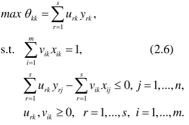
. The

638

1

1

1 1

,

s.t.

1,

(2.6)

0,

1,..., ,

,

0,

1,..., ,

1,..., .

s

kk rk rk

r m

ik ik i

s s

rk rj ik ij

r r

rk ik

max

u y

v x

u y

v x

j

n

u

v

r

s i

m



   

























WhereDMU_k is the DMU under evaluation,



1,...,



ik

v i m and u_rk



r1,...,s



are input

and output weights. Let u_rk



r1,...,s



and



1,...,



ik

v i m be the optimal solution to the

above CCR model. Then,

1 s

kk rk rk

r

u y



 







is

referred to as the CCR-efficiency ofDMU_k,

which is the best relative efficiency of DMUk

by self-evaluation. If



_kk 1, DMU_k is said to be CCR-efficient; otherwise, it is said to be non-CCR-efficient.

1 1

s m

jk _r

u y

rk rj _i

v x

ik ij



 

 







is referred to as

the cross-efficiency of DMU_ktoDMU_j by

peer-evaluation, where

j



1,..., ;

n j



k

.

Model (2.6) is solved n times, each time for one particular DMU. As a result, we can get one CCR-efficiency value and



n1



cross-efficiency values for each DMU. The n efficiency values constitute a cross-efficiency matrix, as shown in table (2.1), where



1,...,



kk k n



 are the CCR-efficiency

values of the n DMUs, i.e.



_kk 



_kk . The n

efficiency values of each DMU are then simply averaged as its overall performance, which is called average cross-efficiency value. Based on these overall performance values, the n DMUs can be compared or fully ranked.

Table 2.1 cross-efficiency matrix for n DMUs D

M U

Target DMU average

crosses efficiency

1 2 … n

1

11



12



… 1n ₍1₎ 1 1 n n k k    2 21

 ₂₂

… 2n ₍1₎ 2 1 n n k k    . . . . . . . . . … . . . n 1 n  _n2

… nn _{( )}1 1 n n nk k   

The above approach about cross-efficiency value in CCR efficiencies or constant returns to scale (CRS) DEA model was extended to the variable returns to scale (VRS) DEA model [25]. The VRS DEA model can generate negative cross-efficiency scores. The VRS DEA model is as follows [1]:

0 1 0 1 1 1 0

max

. .

0,

1,...,

1

(2.7)

u

0,

1,...,

0,

1,...,

0

s rk rk r s m

rk rj ik ij

r i m ik ik i rk ik

u y

u

s t

u y

v x

u

j

n

v x

r

s

v

i

m

weights(u*rk,v*rk). Using this set of weights, the DMUk-based cross efficiency for any



1,...,



j

DMU j n is calculated as

0 1

1

1

(2.8)

k,

1, 2,...,

(

1,..., )

1

(2.9)

s rk rj r kj m ik ij i kj n j kj k

u y

u

E

v x

j

n

The average of all E

k

n

E

E

n

    

















Is used as the cross-efficiency score for



1,...,



j

DMU j n .

Note that the cross-efficiency score obtained in the above manner can be negative. This subject is presented by a simple numerical example involving five DMUs, with two input and single output [25].

The negative VRS cross-efficiency score is

due to the fact that



s_r1

u y

_{rk rj}

 

u

₀

0

for someDMU_j, i.e., some DMU_j will have

negative efficiency ratios when they use a set of optimal weights obtained when DMU_k is under evaluation. Naturally, we want every output-input efficiency ratio be positive regardless of the chosen weights. Therefore,

adding



s_r1

u y

_{rk rj}

 

u

₀

0

into the VRS model is proposed when calculating the cross-efficiency scores [25]. This will also guarantee non-negativity of both VRS cross-efficiency scores and VRS efficiency ratios.

Therefore the following modified VRS DEA model is used for model (2.7) development and application: 0 1 0 1 1 1 0 1 0

max

. .

0,

1,...,

1

0,

1, 2,..,

(2.10)

u

0,

1,...,

0,

1,...,

0

s rk rk r s m

rk rj ik ij

r i m ik ik i s rk rj r rk ik

u y

u

s t

u y

v x

u

j

n

v x

u y

u

j

n

r

s

v

i

m

u

    







































2.3 Cross-efficiency in the presence of

negative data

In the conventional DEA models, each

(

1,..., )

j

DMU

j



n

is specified by a pair of

non-negative input and output vectors

( ,

x y

_{j j}

)



R

m s , in which inputs

(

1,..., )

ij

x i



m

are utilized to produce outputs,

(

1,..., )

rj

y r



s

. These models cannot be used

640

1

1

1

max

. .

1,..., ,

1,..., ,

1,

(2.11)

0

1,..., .

n

j ij io io

j n

j rj ro ro

j n

j j

j

s t

x

x

R

i

m

y

y

R

r

s

j

n















  

























Ideal point (

I

) in the presence of negative

data, is

(max {

_{j rj}

:

1,..., }, min {

_{j ij}

:

1,..., }

I



y

r



s

x

i



m

where

,

min {

:

1,..., },

1,...,

,

max {

:

1,..., }

1,..., .

(2.12)

io io j ij

ro j rj ro

R

x

x

j

n

i

m

R

y

j

n

y

r

s

















The other models solve negative data such as Modified slacks-based measure model (MSBM), semi-oriented radial measure (SORM) and etc.

In this section, we define cross-efficiency in the presence of negative data under variable returns to scale (VRS). In financial literature, mean – variance model and mean-variance-skewness are proposed based on Data Envelopment Analysis, which the variance of the portfolios is used as an input to the DEA and expected return and skewness are the output. Thus, we know that unlike return and skewness, variance is the only variable in the model that takes non-negative values. In this paper, new cross-efficiency is introduced based on RDM model.

Definition 2.1

m s

* *

io ij ro rj 0

i 1 r 1

jo jo m s

* *

io ij ro rj

i 1 r 1

v x

u y

u

1

1

v R

u R

(2.13)





   





 

 











is referred to as the cross-efficiency of DMUo

to

DMU

_jby peer-evaluation, with negative data, where

j 1,..., n; j





o

.

In the above mentioned ratio,DMU_o is the

DMU under evaluation and

u

_ro



r



1,...,

s



and

v

_io



i



1,...,

m



are the optimal solution to

the below model. Thus,

x

_ij



1,...,

m



and



1,...,



rj

y

r



s

are the input and output

values of

DMU

_j



j



1,...,

n



m s

i io r ro 0

i 1 r 1

m s

i ij r rj 0

i 1 r 1

m s

i io r ro

i 1 r 1

i r

min

v x

u y

u

s.t.

v x

u y

u

0

(2.14)

v R

u R

1

v

0 u

0 i 1,..., m r

1,...,s

     



































The above model is RDM model dual. Model (2.14) can be stated as follows:

s m

r ro i io 0

r 1 i 1

m s

i ij r rj 0

i 1 r 1

m s

i io r ro

i 1 r 1

i r

max

u y

v x

u

s.t.

v x

u y

u

0

(2.15)

v R

u R

1

v

0 u

0 i 1,..., m r

1,...,s

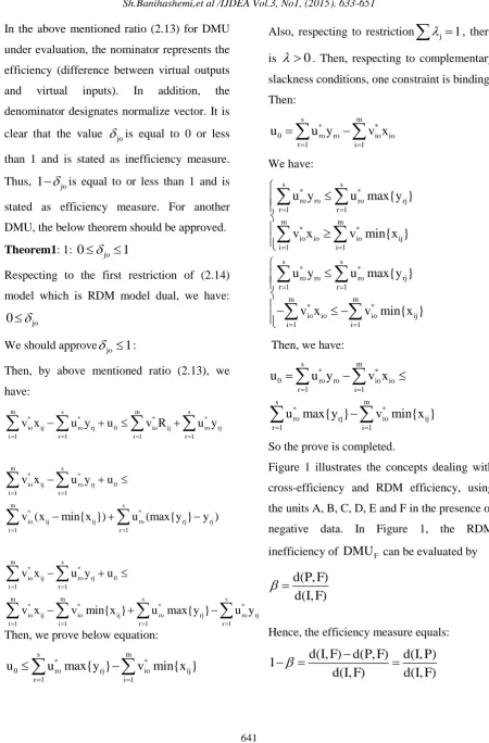
In the above mentioned ratio (2.13) for DMU under evaluation, the nominator represents the efficiency (difference between virtual outputs and virtual inputs). In addition, the denominator designates normalize vector. It is clear that the value



_jois equal to 0 or less

than 1 and is stated as inefficiency measure. Thus,

1





_jois equal to or less than 1 and is stated as efficiency measure. For another DMU, the below theorem should be approved. Theorem1: 1:

0





_jo



1

Respecting to the first restriction of (2.14) model which is RDM model dual, we have:

jo

0





We should approve



_jo



1

:

Then, by above mentioned ratio (2.13), we have:

m s m s

* * * *

io ij ro rj 0 io ij ro rj i 1 r 1 i 1 r 1

m s * *

io ij ro rj 0 i 1 r 1

m s

* *

io ij ij ro rj rj i 1 r 1

m s * *

io ij ro rj 0 i 1 r 1

m m s

* * *

io ij io ij ro i 1 i 1 r 1

v x u y u v R u y

v x u y u

v (x min{x }) u (max{y } y )

v x u y u

v x v min{x } u m

                           



























s

* rj ro rj

r 1

ax{y } u y







Then, we prove below equation:

s m

* *

0 ro rj io ij

r 1 i 1

u

u max{y }

v min{x }

 









Also, respecting to restriction





_j1, there

is





0

. Then, respecting to complementary slackness conditions, one constraint is binding. Then:

s m

* *

0 ro ro io io

r 1 i 1

u

u y

v x

 









We have:

s s

* *

ro ro ro rj

r 1 r 1

m m

* *

io io io ij

i 1 i 1

s s

* *

ro ro ro rj

r 1 r 1

m m

* *

io io io ij

i 1 i 1

u y

u max{y }

v x

v min{x }

u y

u max{y }

v x

v min{x }

       

























 



















Then, we have:

s m

* *

0 ro ro io io

r 1 i 1

s m

* *

ro rj io ij

r 1 i 1

u

u y

v x

u max{y }

v min{x }

   

















So the prove is completed.

Figure 1 illustrates the concepts dealing with cross-efficiency and RDM efficiency, using the units A, B, C, D, E and F in the presence of negative data. In Figure 1, the RDM inefficiency of DMU_F can be evaluated by

d(P, F)

(2.16)

d(I, F)





Hence, the efficiency measure equals:

d(I, F) d(P, F)

d(I, P)

1

(2.17)

d(I, F)

d(I, F)





 



642 Equation (2.17) represents the RDM efficiency of DMU_Fwhich is between 0 and 1.

d(I, F)

and

d(I, P)

denote the distance from the ideal point

I

to

F

and the distance from the ideal point

I

to

P

, respectively, and

d(P, F)

is the distance from

P

to

F

.

Figure1: RDM and BCC frontier in the presence of negative data

I is the ideal point. Using Figure 1, it is easy to see that the efficiency measure yielded by model RDM,1





, is a distance measure between the observed and its target point

P

with reference to the ideal point.

2.4 OWA operators and their weight

determination methods

An OWA operator of dimension n is a mapping

F

:

 

n with an associated weight vector

W





w

₁

,...,

w

_n



T such that

1 ... n 1, i 1, 1,..., .

w  w  ow  i n

And

1

1

( ,..., ) , (2.18)

n

n i i

i

F a a w b







Where b_iis the ith largest ofa₁,...,a_n .

OWA operators, introduced by yager [26], provide a unified framework for decision making under uncertainty, where different decision criteria such as maximax (optimistic), maximin (pessimistic), equally likely (Laplace) and Hurwicz criteria are characterized by different OWA operator weights.

For different weight selections, they are distinguished by the following orness degree [26]:

 





1

1

(2.19) 1

n

i i

orness W n i w

n 

 





The orness degree can be regarded as a measure of the optimism level of the DM. To apply OWA operators for decision making, it is essential to determine the weights of OWA operators. The following models (2.20) and (2.21) are two important approaches for determining OWA operator weights under a given orness degree:

 

 





n

i i

i=1

1

1

max Disp W =

w lnw ,

1

s.t. orness W =

, 0

1,

1

1,

(2.20)

0,

1,..., .

n

i i

n i i

i

n

i w

n

w

w

i

n













 















 





1

1

1

1

min δ

s.t.

1

orness W

, 0

1,

1

1,

0,

1,...,

1,

(2.21)

0,

1,...,

1,

0,

1,..., .

n

i i

n i i

i i

i i

i

n i w

n

w

w

w

i

n

w

w

i

n

w

i

n











  

 



 







 







 













Model (2.20), suggested by O’Hagan [14] maximizes the entropy of weight distribution and is thus referred to as the maximum entropy method, whereas model (2.21) that was proposed by Wang and Parkan [21] minimizes the maximum disparity between two adjacent weights and is thus called the minimax disparity approach.

The OWA operator weights determined by the above models have the following characteristics:

The weights are ordered. That is

1 2 ... n 0

w w  w  if the orness degree

0.5





and 0w₁w₂  ... w_nif

0.5





.

The weights have nothing to do with the magnitudes of the aggregates , but depend upon their ranking orders and the DM’s optimism level (orness degree).

1 1

w  andwj 0 (j1) if





1

.Which means that the DM or investor is purely optimistic and considers only the biggest value

 

1 maxi i

b  a in decision analysis.

1

n

w  andwj 0 (jn) if





0

, which represents that the DM or investor is purely pessimistic and is only concerned with the most conservative value bn mini

 

ai when

making decision.





1 ... n 1/

w  w  n if





0.5

, which stands for that the DM or investor is neutral and makes use of all the aggregates equally in decision making.

1,..., n

w w determined by model (2.20) vary in

the form of geometric progression, i.e.

1

i i

w_ w q for

i



1,...,

n



1

, where

q



0

, while w1,...,wn determined by model (2.21)

vary in the form of arithmetical progression,

namely, wiwi1 d for





1,...,

i K Kn or w_i1w_i d for





,..., 1

iK n K where

d



0

.

3. Methodology

644 investors prefer skewness which means that utility functions of investors are not quadratic. Thus, we know that unlike return and skewness, variance is the only variable in the model that takes non-negative values. The methodology in this paper starts with asset selection via cross-efficiency evaluation in presence of negative data using OWA operator weights. The data used for this methodology is from 20 Iranian stock companies. In many cases similar to this example there are a lot of assets. It is better that starts with asset selection. The choice of the asset can be random or discrete. The random choice of assets is usually biased and do not promise an optimum portfolio; hence it is more rational to have an objective choice while selecting the assets to be included in the portfolio. Among many evaluation methods, Data Envelopment Analysis (DEA) is one of the best ways for assessing the relative efficiency a group of homogenous decision making units (DMUs) that use multiple inputs to produce multiple outputs, originated from the work by charnes et al. [2]. Cross-efficiency evaluation is effective way of ranking decision making units (DMUs). It allows the overall efficiencies of the DMUs to be evaluated through self- and peer-evaluations. The self-evaluation allows the efficiencies of the DMUs to be evaluated with the most favorable weights so that each of them can achieve its best possible relative efficiency, whereas the peer-evaluation requires the efficiency of each DMU to be

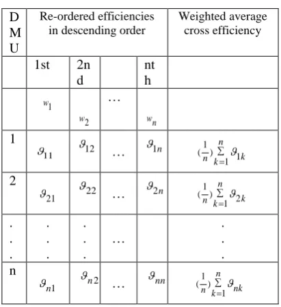
evaluated with the weights determined by the other DMUs. Table (3.1) shows cross-efficiency matrix for n DMUs with negative data. Traditional approaches for the cross-efficiency evaluation do not differentiate between self-evaluated and peer-evaluated efficiencies. A significant problem with these approaches is that the weight assigned to the self-evaluated efficiency of each DMU is fixed and has no way of incorporating the DM’s or investor’s subjective preferences in to the evaluation. For example, the investors may wish self-evaluated efficiencies to account for 20% or play a leading role in the final overall efficiency assessment. Obviously, equal evaluation has no method to obtain this purpose. To show the investor’s subjective preferences on different efficiencies, the use of OWA operator weights is stated for cross-efficiency evaluation. This requires the re-ordering of the efficiencies, both self-evaluated and peer-self-evaluated, of each DMU, as shown in Table (3.2), where w1,...,wnare

OWA operator weights,



ij( ,i j1,..., )n are

re-ordered efficiencies of each DMU from the biggest to the smallest. Obviously, self-evaluated efficiencies are always ranked in the first place, i.e. *

1 1,...,



_i 



_iii n. In order to

the self-evaluated efficiencies to account for 20% in the final overall efficiency assessment, then w1should take 0.2, whereas the other weights can be designated minimax disparity approach. The orness degree can be regarded as a measure of the optimism level of the investor. If the investor wants to self-evaluated to be more influenced, it should be used of orness> 0.5. And if investor wants to peer-evaluated to be more influenced, it should be used of orness< 0.5. Obviously, the best selection of stocks is not fixed. It varies with the investor’s optimism level or subjective performance.

Table 3.1. cross-efficiency matrix for n DMUs with negative data

D M U

Target DMU average crosses efficiency with negative data

1 2 … n

1

11

 ₁₂

…

1n

 1

( ) ₁

1 n

n k k  2

21  ₂₂

… 2n _{( )}1

2 1 n

n k k 

. . . . . . . . . … . . . n 1 n

 _n2

… nn _{( )}1

1 n

n nk k 

Table 3.2. Re-ordered cross-efficiency matrix of the n DMUs

D M U

Re-ordered efficiencies in descending order

Weighted average cross efficiency

1st 2n d nt h w1 2 w … wn 1 11

 12

…

1n

 1

( ) ₁ 1 n n k k    2 21  22 

… 2n ₍1₎ 2 1 n n k k    . . . . . . . . . … . . . n 1 n

 n2 _… nn _{( )}1

1 n n nk k   

4. Application in Stocks Company

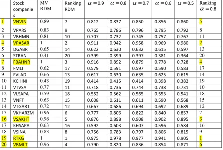
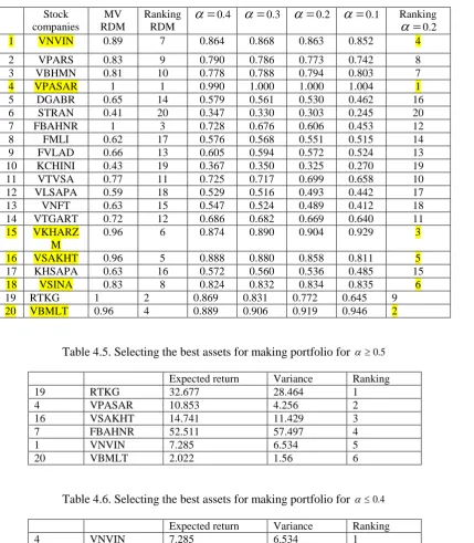
646 Equation (2.13) is used for efficiency evaluation. In the analysis, the variance of the stocks is used as an input to the DEA and expected return is used as an output. Traditional approaches for the cross-efficiency evaluation do not differentiate between self-evaluated and peer-self-evaluated efficiencies. A main problem with these approaches is that the weight assigned to the self-evaluated efficiency of each DMU is fixed and has no way of incorporating the investor’s subjective preferences in to the evaluation. Obviously, equal evaluation has no way to obtain this goal. To show the investor’s subjective preferences on different efficiencies, the use of OWA operator weights is stated for cross-efficiency evaluation in Table (4.2). This requires the re-ordering of the efficiencies. The orness degree can be regarded as a measure of the optimism level of the investor. If the investor wants to self-evaluated to be more influenced, it should be used of orness> 0.5. And if investor wants to peer-evaluated to be more influenced, it should be used of orness< 0.5. In the traditional equal of cross-efficiencies, the weight assigned to the

self-evaluated efficiencies is only 0.05% 1

20















.

For an optimistic investor, he/she may wish the self-evaluated efficiencies to play a more role in the final overall efficiency assessment. For example, the investor may wish the weight for the self-evaluated efficiencies to account for 20% rather than 0.05% in the final overall

efficiency assessment. As it seen in Tables (4.3), (4.4) ranks are not the same. We calculated these ranks for o.8 and0.2. Some of the best ranks are designated according to investor. We consider six of the best ranks. Selecting of stocks to be included in portfolio is followed by six of the best ranks in Tables (4.5), (4.6) for 0.5 ,0.4, respectively.

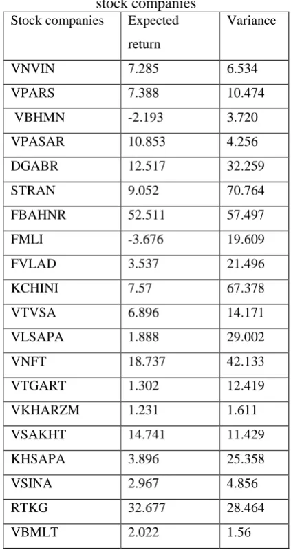
Table 4.1. Descriptive statistics of the Iranian stock companies

Stock companies Expected return

Variance

VNVIN 7.285 6.534

VPARS 7.388 10.474

VBHMN -2.193 3.720

VPASAR 10.853 4.256

DGABR 12.517 32.259

STRAN 9.052 70.764

FBAHNR 52.511 57.497

FMLI -3.676 19.609

FVLAD 3.537 21.496

KCHINI 7.57 67.378

VTVSA 6.896 14.171

VLSAPA 1.888 29.002

VNFT 18.737 42.133

VTGART 1.302 12.419

VKHARZM 1.231 1.611

VSAKHT 14.741 11.429

KHSAPA 3.896 25.358

VSINA 2.967 4.856

RTKG 32.677 28.464

Table 4.2. OWA operator weights for cross efficiency evaluation





0.9





0.8





0.7





0.6





0.5





0.4





0.3





0.2





0.1

0.9 0.8 0.7 0.6 0.5 0.4 0.3 0.2 0.1

0.261 0.149 0.105 0.077 0.05 0.023 0 0 0

0.221 0.137 0.099 0.074 0.05 0.026 0 0 0

0.182 0.125 0.093 0.071 0.05 0.029 0.006 0 0 0.143 0.113 0.087 0.069 0.05 0.031 0.012 0 0 0.104 0.101 0.082 0.066 0.05 0.034 0.018 0 0 0.064 0.089 0.076 0.063 0.05 0.037 0.024 0 0 0.025 0.077 0.07 0.06 0.05 0.04 0.029 0 0 0 0.065 0.064 0.057 0.05 0.043 0.035 0.004 0 0 0.053 0.058 0.054 0.05 0.046 0.041 0.016 0 0 0.041 0.053 0.051 0.05 0.049 0.047 0.029 0 0 0.029 0.047 0.049 0.05 0.051 0.053 0.041 0 0 0.016 0.041 0.046 0.05 0.054 0.058 0.053 0 0 0.004 0.035 0.043 0.05 0.057 0.064 0.065 0

0 0 0.029 0.04 0.05 0.06 0.07 0.077 0.025

0 0 0.024 0.037 0.05 0.063 0.076 0.089 0.064 0 0 0.018 0.034 0.05 0.066 0.082 0.101 0.104 0 0 0.012 0.031 0.05 0.069 0.087 0.113 0.143 0 0 0.006 0.029 0.05 0.071 0.093 0.125 0.182

0 0 0 0.026 0.05 0.074 0.099 0.137 0.221

0 0 0 0.023 0.05 0.077 0.105 0.149 0.261

Table 4.3. Cross efficiency by optimism level of the investor for 0.5

Stock companie s

MV RDM

Ranking RDM





0.9





0.8





0.7





0.6





0.5 Ranking





0.8

648

Table 4.4. Cross efficiency by OWA operator weights for  0.4 Stock

companies

MV RDM

Ranking RDM





0.4





0.3





0.2





0.1 Ranking





0.2

1 VNVIN 0.89 7 0.864 0.868 0.863 0.852 4

2 VPARS 0.83 9 0.790 0.786 0.773 0.742 8

3 VBHMN 0.81 10 0.778 0.788 0.794 0.803 7

4 VPASAR 1 1 0.990 1.000 1.000 1.004 1

5 DGABR 0.65 14 0.579 0.561 0.530 0.462 16

6 STRAN 0.41 20 0.347 0.330 0.303 0.245 20

7 FBAHNR 1 3 0.728 0.676 0.606 0.453 12

8 FMLI 0.62 17 0.576 0.568 0.551 0.515 14

9 FVLAD 0.66 13 0.605 0.594 0.572 0.524 13

10 KCHINI 0.43 19 0.367 0.350 0.325 0.270 19

11 VTVSA 0.77 11 0.725 0.717 0.699 0.658 10

12 VLSAPA 0.59 18 0.529 0.516 0.493 0.442 17

13 VNFT 0.63 15 0.547 0.524 0.489 0.412 18

14 VTGART 0.72 12 0.686 0.682 0.669 0.640 11

15 VKHARZ M

0.96 6 0.874 0.890 0.904 0.929 3

16 VSAKHT 0.96 5 0.888 0.880 0.858 0.811 5

17 KHSAPA 0.63 16 0.572 0.560 0.536 0.485 15

18 VSINA 0.83 8 0.824 0.832 0.834 0.835 6

19 RTKG 1 2 0.869 0.831 0.772 0.645 9

20 VBMLT 0.96 4 0.889 0.906 0.919 0.946 2

Table 4.5. Selecting the best assets for making portfolio for  0.5 Expected return Variance Ranking

19 RTKG 32.677 28.464 1

4 VPASAR 10.853 4.256 2

16 VSAKHT 14.741 11.429 3

7 FBAHNR 52.511 57.497 4

1 VNVIN 7.285 6.534 5

20 VBMLT 2.022 1.56 6

Table 4.6. Selecting the best assets for making portfolio for 0.4 Expected return Variance Ranking

4 VNVIN 7.285 6.534 1

20 VBMLT 2.022 1.56 2

15 VKHARZM 1.231 1.611 3

1 VNVIN 7.285 6.534 4

16 VSAKHT 14.741 11.429 5

5. Conclusion

In this paper, a new method is suggested for selecting the best of portfolio with one input (variance) and one output (expected return) in the DEA context in presence negative data. The cross-efficiency evaluation is an important method for ranking DMUs in DEA. Traditional approaches for the cross-efficiency evaluation do not differentiate between self-evaluated and peer-self-evaluated efficiencies. A main problem with these approaches is that the weight assigned to the self-evaluated efficiency of each DMU is fixed and has no way of incorporating the investor’s subjective preferences in to the evaluation. To show the investor’s subjective preferences on different efficiencies, the use of OWA operator weights is stated for cross-efficiency evaluation. In this case, if the investor wants to self-evaluated to be more influenced, it should be used of orness> 0.5. Thus, if investor wants to peer-evaluated to be more influenced, it should be used of orness< 0.5. In Tables 8,9 rankings have been designated for six of the best stocks via OWA operator weights in cross-efficiency evaluation in presence negative data. Since there are a large number of assets to invest in, this objective leads to two investment problems. First, the assets are selected for making portfolio and second, the proportion or weights are determined to be allocated to the selected assets. Selection of assets to be included in portfolio is followed by using cross-efficiency evaluation. Model (2.10) is

used for this purpose. In this regard, this model is used to analyze the given 20 Iranian stock companies and six of the best stocks are obtained.

Acknowledgement

The authors’ sincere thanks go to the known and unknown friends and reviewers who meticulously covered the article and provided us with valuable insights.

Reference

[1] D. Banker, A. Charnes , W.W. Cooper, Some models for estimating technical and scale inefficiencies in data envelopment analysis, Management Science 30 (1984) 1078 1092.

[2] A. Charnes, W. W. Cooper , E. Rhodes, Measuring Efficiency of Decision Making Units. European Journal of Operational Research 2 (1978) 429–444.

[3] A. Charnes, W.W. Cooper, A. Y. Lewin, L. M. Seiford, Data Envelopment Analysis: Theory, Methodology and Applications, Kluwer Academic Publishers, Boston.(1994). [4] J. Doyle, R. Green. Efficiency and cross-efficiency in DEA, derivations, meanings and uses, Journal of the Operational Research Society 45 (1994) 567-578.

[5] JR. Doyle, RH. Green, Cross-evaluation in DEA: improving discrimination among DMUs, INFOR 33 (1995) 205–22.

650 using DEA, European journal of Operational Research, 200 (2010) 297-304.

[7] RH. Green, JR. Doyle, WD. Cook, Preference voting and project ranking using DEA and cross-evaluation. European Journal of Operational Research 90 (1996) 461–72. [8] T. Joro, P. Na, Portfolio performance evaluation in a mean-variance-skewness framework. European Journal of Operational Research 175 (2005) 446–461.

[9] L. Liang, J. Wu, WD. Cook, J. Zhu, The DEA game cross-efficiency model and its Nash equilibrium. Operations Research 56 (2008) 1278–88.

[10] WM. Lu, SF. Lo. A closer look at the economic-environmental disparities for regional development in China. European Journal of Operational Research 183 (2007) 882–94.

[11] WM. Lu, SF. Lo, A benchmark-learning roadmap for regional sustainable development in China. Journal of the Operational Research Society 58 (2007) 841–9.

[12] H. M. Markowitz, Portfolio selection, Journal of Finance 7 (1957) 77–91.

[13] M. R. Morey, R. C. Morey, Mutual fund performance appraisals: A multi-horizon perspective with endogenous benchmarking. Omega 27 (1999) 241–258.

[14] M. O’Hagan, Aggregating template or rule antecedents in real-time expert systems with fuzzy set logic, In: Proceedings of the 22nd annual IEEE Asilomar conference on

signals, systems and computers, Pacific Grove, California (1988) p. 681–9.

[ 51

] M. C. Portela‎, e.‎‎‎ Thanassoulis‎, ‎G.‎‎‎ Simpson‎, ‎‎ ‎A directional distance approach to deal with negative data in DEA‎ : ‎An application to bank branches‎, ‎Journal of Operational Research Society 55 (2004‎)‎ ‎1111-1121‎.

[16] JA. Sharp, W. Meng, W. Liu, A modified slacks-based measure model for data envelopment analysis with ‘natural’ negative outputs and inputs, Journal of the Operational Research Society (2006) 571-6.

[17] TR. Sexton, RH. Silkm, AJ. Hogan, Data envelopment analysis: critique and extensions, Measuring efficiency: an assessment of data envelopment analysis, San Francisco, CA: Jossey-Bass (1986) p. 1986.

[18] W.F. Sharpe, Capital asset prices: A theory of market equilibrium under conditions of risk, Journal of Finance 19 (1964) 425–442. [19] W.F. Sharpe.“Investment”, Third Edition, Prentice-Hal, envelopment analysis, Management Science, 30 (1985) 1078 1092. [20] Y. Wang, k. Chin, The use of OWA operator weights for cross-efficiency aggregation, Omega, 39 (2011) 493-503. [21] YM, Wang, C. Parkan, A minimax disparity approach for obtaining OWA operator weights, Information Sciences 175 (2005) 20–9.

efficiency model, Journal of the Operations Research Society of Japan 52 (2009) 105–11. [23] J. Wu, L, Liang, D. Wu, F. Yang, Olympics ranking and benchmarking based on cross efficiency evaluation method and cluster analysis: the case of Sydney 2000, International Journal of Enterprise Network Management 2 (2008) 377–92.

[24] J, Wu, L, Liang, F. Yang, Achievement and benchmarking of countries at the Summer Olympics using cross efficiency evaluation method, European Journal of Operational Research 197 (2009) 722–30.

[25] J.Wu, L. Liang, Y. Chen, DEA game cross-efficiency approach to Olympic rankings, Omega 37 (2009)909–18.