ORIGINAL PAPER
Investigation of the performance and accuracy of multivariate time
series models in predicting electrical conductivity and total
dissolved solid values of the rivers of Urmia lake basin
Mohammad Soleimani1 , Keivan Khalili2, , Javad Behmanesh3
1. Ph.D. in Water Science and Engineering, Directorate of Piranshahr health center, Urmia University of Medical Sciences, Jahad Ave., Urmia, Iran
2. Assistant Professor, Department of Water Engineering, University of Urmia, Urmia, Iran 3. Associate Professor, Department of Water Engineering, University of Urmia, Urmia, Iran
Date of submission: 21 Jan 2017, Date of acceptance: 20 May 2017
ABSTRACT
Considering the complexity of hydrological processes, it seems that multivariate methods may enhance the accuracy of time series models and the results obtained from them by taking more influential factors into account. Indeed, the results of multivariate models can improve the results of description, modeling, and prediction of different parameters by involving other influential factors. In this study, univariate models (ARMA) and auto-correlated multivariate models with the simultaneous autoregressive moving average model (CARMA) were evaluated for modeling Electrical Conductivity and Total Dissolved Solid parameters of the western stations of Urmia Lake Basin. To use the CARMA models, annual flow rate time series, EC, TDS, SAR, and pH values measured across seventeen hydrometric stations between 1992 and 2013 were used. In the studied statistical period, the river flow in the west of Urmia Lake Basin decreased and experienced an incremental increase compared to the EC and TDS values in river flow. By applying influential parameters in CARMA models, the mean error value of the model in training and experimental stages reduces by 32% and 44% for EC values and 34% and 36% for TDS values, respectively.
Keywords: Time series model, ARMA, CARMA, water quality, Urmia Lake
Introduction
Predicting hydrological parameters has always been of interest to water engineers, owing to their significance in the analysis of drought and water supply, such as designing
water establishments, river dewatering,
planning for exploiting the reservoirs of dams, and controlling erosion and sedimentation of rivers. Considering how restricted the use of exploitable freshwater resources is, accurate prediction of the flow rate of hydrological parameters is one of the primary bases of planning and managing water resources. Water quality modeling is one of the major interests of water experts because it can directly influence human’s life.1 Electrical Conductivity and Total
Khalili Keivan [email protected]
Citation: Soleimani M, Khalili K, Behmanesh J. Investigation
of the performance and accuracy of multivariate time series models in predicting Electrical Conductivity and Total Dissolved Solid values of the rivers of Urmia Lake Basin. J Adv Environ Health Res 2017; 5(3): 131-138
Dissolved Solid values are both the important parameters in water quality.2 This paper outlines the modeling of these two issues. Several authors have attempted to predict these parameters like3 modeling EC on ground water,1 Karamouz for river water quality,4 Orouji et.al on water quality.5 Accordingly, experts are always developing models to better estimate river flow rates accurately, modified from current methods.2,5–8 So, far, various models
have been proposed to simulate hydrological and meteorological parameters of an area through deterministic modeling. For example, one can mention precipitation-runoff conceptual models, time series linear patterns, genetic
programming, and hybrid combinational
models.The first group of models is based on physical characteristics of the system, presented
in the form of differential equations.
characteristics of the hydrological system of interest; precipitation-runoff models belong to this group. Some experimental models attempt to develop a relationship between input and output data with no consideration of physical parameters. These models are known as black box models. This group of models can include the experimental relationships of estimation of focus time and interception calculation models. The first application of linear models for time series in hydrology was performed by Thomas and Firing.9 These models include the autoregressive moving average model (ARMA) ,10 with constant parameters, and the models
derived from it, including autoregressive models (AR), moving average (MA) and cumulative autoregressive moving average1 (ARIMA), which together use methods for estimating the model parameters and goodness of fit. Furthermore, periodic models in which the model's parameters are not constant were introduced and presented four processes in which a periodic characteristic is observed in the
parameters, including the periodic
autoregressive models (PAR) and periodic
autoregressive moving average model
(PARMA). Zou et al compared two models:
ARIMA and the artificial neural network for predicting water capacity and soil salt.11 They showed that the ARIMA model resulted in greater accuracy. Investigating the review of the literature, it seems that multivariate time series models, such as CARMA, have not been used in modeling of qualitative parameters. The aim of this research is to model qualitative parameters of Urmia Lake Rivers within the period of 1992–2013.
northwest of Iran between 35° and 58' until 39° and 46' of northern latitude and 44° and 3' until 47° and 23' of eastern longitude. The area of this basin, taking Urmia Lake into account, is 43,660 km2. The Basin of Urmia Lake is one of the most important regional basins of Iran, situated in the northwest of Iran. This basin, with an area of 52,700 km2 and accounting for 3.21% of the entire country's area, lies between 35° and 40' until 38° and 29' of northern latitude and the meridian of 44° 13' and 47° 53' of eastern longitude. The position of the stations studied across western Azerbaijan Province is shown in Fig1.
Fig. 1. Location of the study area in the region, Iran and the location of 17 hydrometric stations studied
1
Autoregressive Integrated Moving Average
The studied regions
The statistical specifications of the applied data are presented in Table 1. The 17 hydrometric stations of Iran with their elevation
and also geographic properties are shown in this table.
Table 1. Specifications of hydrometric stations used in this study Station
number Station
Elevation (m)
Geographic properties
X Y
1 Abajalo 1280 -14887.763 4191113.096
2 Alasagel 1700 145621.718 4045364.055
3 Babarood 1283 -7710.074 4155233.042
4 Balegchi 1350 -1938.191 4102023.035
5 Bitas 1408 26194.05 4071683.848
6 Chehriq 1520 -62376.418 4234508.762
7 Ghasemlo 1340 -18412.351 4149635.085
8 Gerdyaghob 1280 30105.376 4107642.735
9 Hashemabad 1447 -37821.81 4145565.016
10 Kotar 1360 19675.413 4076349.532
11 Oshnaviyeh 1471 -25770.773 4116232.916
12 Pey-gale 1487 -31187.653 4111057.45
13 Pol-Anian 1425 88485.401 4016034.688
14 Pol-Miandoab 1290 59386.185 4101951.86
15 Sari Ghamish 1380 96363.496 4046881.692
16 Tapik 1380 -38605.124 4188292.51
17 Urban 1700 -49348.359 4261336.985
Materials and Methods
ARMA multivariate models
There are various methods required in the analysis and modeling of hydrological time series. The characteristic of certain concurrent models is diagonal parameter matrices, whose estimation of its parameters is independent of univariate models. Among multivariate linear models12 are a multivariate auto-regressive model (MAR) (p), concurrent ARMA, known as CARMA, combinational model of concurrent and moving average (CARMA) (p,q), known as
CSM-CARMA (p,q), and a seasonal
multivariate auto-regressive periodic model
(MPAR)(p). Modeling of multivariate
hydrological processes based on the complete multivariate model of ARMA often develops problems in the estimation of its parameters. The CARMA model was suggested as a simpler substitute for the complete multivariate ARMA model. 13 In the CARMA (p,q) model, the matrix of the parameters of both auto-regressive and moving average models are assumed to be diagonal, whereas a multivariate model can be considered to be independent of the univariate ARMA model. Therefore, instead of estimating
the model's parameters jointly, they can be estimated independently for every univariate ARMA site. This results in the identification of the best univariate ARMA model. Therefore, if a complete multivariate ARMA model is used, then the different dependence structures in time can be considered a similar dependent structure in time for all sites, instead of modeling it for every site.
The CARMA (p,q) model for n sites can be shown as follows:
(1)
ε
θ
ε
Y
φ
Y
t jq 1 j j _
t p
1
i j t j
t =
∑
= _ +∑
= _Where, Yt is a n*1 column matrix from the
observational series of Ykt with a normal
distribution and means of zero as a representative of different sites of k = 1,2,…, n. Then, φ1,φ2,…,φn is a n*n diagonal matrix of the
parameters of the autoregressive model and θ1,
θ2,…, θq is the n*n diagonal matrix of the
parameters of the moving average model. εt is
also a n*1 matrix of normal random data with a mean of zero and variance-covariance of g.
[ Yt
(1)
Yt(2) . . . 𝑌𝑡(𝑛)]
=
[
φ11 φ12 . . . φ1n φ21 φ22 . . . φ2n . . . . . . . . . φ𝑛1 φ𝑛2 . . . φnn
]
[ Yt−1
(1)
Yt−1(2) . . . 𝑌𝑡−1(𝑛)]
+
[
θ11 θ12 . . . θ1n θ21 θ22 . . . θ2n . . . . . . . . . θ𝑛1 θ𝑛2 . . . θnn]
[ εt(1) εt(2) . . . ε𝑡(𝑛)]
(2)
interactive correlation zero delays across different sites. In addition, the dependence of time structure for each site has been defined by p and q parameters.13
Estimation of model's parameters
By considering N years of data in every site, i, with observational data of Y(i)t and I = 1,
2,…, n, the matrix of the general model of Yt is
described as follows:
(3)
Z
Y
t= μ+σ tWhere µ and σ are the mean and variance of Yt.
Standardization of variables is calculated by the following relationship: (4) n ,..., 2 , 1 i , / ) _
(
y
μ
σ
Z
(ti) (i) ) i ( t ) i (t = =
The parameters of model CARMA (p(i), q(i)) is determined as with the parameters of the ARMA model. The model's remaining time series is independent of time, but is dependent among itself (is dependent on the space). This interactive dependence can be modeled using the following relationships:
(5)
σ
ε
ε
(i)t ) i ( t ) i ( t =
′
(6)ξ
ε
′
t=B tWhere B is estimated by the following relationship: (7) 0 T M B B =
Where, M0is the matrix of autocorrelation function with zero delays, calculated by the following matrix:
2Root Mean Square Error
(8)
r
r
r
r
r
r
r
r
r
nn k 2 n k 1 n k n 2 k 22 k 21 k n 1 k 12 k 11 k k ... : : : ... ...M =
(9)
∑
∑
∑
= = + + = + + = K N 1 t 2 ) i ( k t ) i ( k t K _ N 1 t 2 ) i ( t ) i ( t K N 1 t ) i ( k t ) i ( k t ) i ( t ) i ( t ij k _ _ ) _ ( . ) _ ( ) _ )( _ (ε
ε
ε
ε
ε
ε
ε
ε
r
Where
ε
(ti)is the mean of N-K data, i, andε
(t+i)k is the N-K mean of data, j. Finally, the matrix of the parameters of model CARMA (p, q) is obtained by the following relationship.14(10) 1 0 1 1 _ Mˆ Mˆ Aˆ =
Evaluation of the model
Two criteria were used to evaluate the performance of the model, the coefficient of determination and root mean square error2 . Greater model accuracy was determined by lower RMSE and higher coefficient of determination values.
𝑅𝑀𝑆𝐸 = √∑𝑇𝑡=1(𝑥̂𝑡− 𝑥𝑡)2
𝑇 (11)
(12)
Where in the above relations xt, 𝑥̂𝑡،, and are the data of observational series, calculated series, and mean, respectively, with T representing the number of data points.
The results of modeling of EC and TDS
Following the primary investigation of the studied data, the results showed that the studied time series data became normalized using logarithm, power, and gamma functions
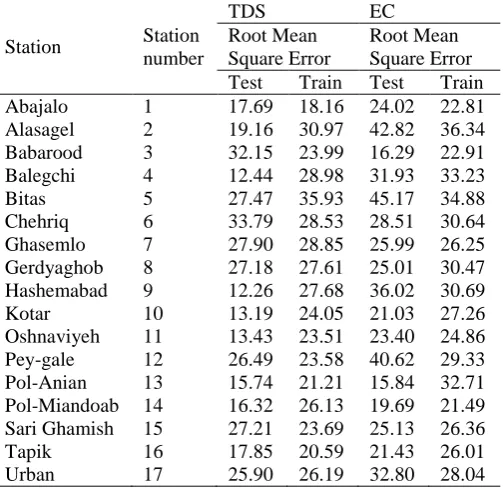
skewness coefficients. First, univariate time series models (ARMA) were investigated. The results indicated that based on Akaike criterion, the ARMA (1, 0) model was chosen for all of the stations. Data are divided for training (calibration of models) and also for testing. Data for this research was obtained from 1992 to 2013. The first 17 years was used to training the model and also considering five years of the data belonging to the end of the study period as the data of the experimental state(testing).To access how the models perform two statistical parameters for accuracy (correlation coefficient) and the model's error (root mean square error) were examined. These results at training and experimental stages are presented in Table 2.
Following an investigation of the univariate models, the normalized data were modeled using multivariate models, considering the mean data of annual flow rate, mean sodium absorption ratio, electrical conductivity, salinity, and pH as input variables. Using the normalized and standardized data under investigation, CARMA (1, 0) model was considered as the best model with the lowest variance among the other models.
As an instance, the parameters and remaining
Table 2. The results of the study and verification of the model ARIMA in modeling EC and TDS values
Station Station
number
TDS EC
Root Mean Square Error
Root Mean Square Error
Test Train Test Train
Abajalo 1 17.69 18.16 24.02 22.81
Alasagel 2 19.16 30.97 42.82 36.34
Babarood 3 32.15 23.99 16.29 22.91
Balegchi 4 12.44 28.98 31.93 33.23
Bitas 5 27.47 35.93 45.17 34.88
Chehriq 6 33.79 28.53 28.51 30.64
Ghasemlo 7 27.90 28.85 25.99 26.25
Gerdyaghob 8 27.18 27.61 25.01 30.47
Hashemabad 9 12.26 27.68 36.02 30.69
Kotar 10 13.19 24.05 21.03 27.26
Oshnaviyeh 11 13.43 23.51 23.40 24.86
Pey-gale 12 26.49 23.58 40.62 29.33
Pol-Anian 13 15.74 21.21 15.84 32.71
Pol-Miandoab 14 16.32 26.13 19.69 21.49
Sari Ghamish 15 27.21 23.69 25.13 26.36
Tapik 16 17.85 20.59 21.43 26.01
Urban 17 25.90 26.19 32.80 28.04
coefficients of CARMA (1, 0) model related to Sari Ghamish Station were presented as Equations (13) and (14), and the Equation of CARMA (1, 0) models were also presented as Equation (15).
) 13 (
1
0.0608617 0.0608617 -0.052516 -0.0064062 0.0360151 0.0608617 0.0608617 -0.052516 -0.0064062 0.0360151 -0.052516 -0.052516 0.118603 -0.0126679 -0.0315455 -0.006406 -0.006406 -0.012667 0.0740856 0.0037688 0.0360151 0.036
A
0151 -0.031545 0.0037688 0.0450799
) 14 (
1
0.246702 0 0 0 0
0.246702 5.26836e-009 0 0 0
-0.212872 -0.00253303 0.270706 0 0
-0.025967 -0.00121162 -0.0672266 0.26247 0
0.145987 0.0017707 -0.00171593 0.0283708 0.151515
B
) 15 (
(1) (1) (2) (3)
1 1 1
(1)
(4) (5)
1 1
0.0608617( ) 0.06017( ) 0.052516( )
0.0064062( ) 0.0360151( ) 0.246702( )
t t t t
t t t
Z
Z
Z
Z
Z
Z
Where(𝑍𝑡−1
(1)
) . (𝑍𝑡−1(2)) . (𝑍𝑡−1(3)) . (𝑍𝑡−1(4)) . (𝑍𝑡−1(5)) 𝑎𝑛𝑑 (𝜀𝑡(1)) are the observation data of the previous period of the values of EC, TDS, flow rate, pH, and SAR, respectively. The results of modeling the EC and TDS values of the hydrometric stations in Urmia Lake basin using CARMA model are
indicated that across all of the studied stations, the accuracy and error of the multivariate time
series model are better than the univariate ARMA model.
Fig. 2. The results of EC and TDS data modeling discussed in Gerd-e Yaghub station
The results of the error and the correlation between historical and modeled data are summarized in Tables 3 and 4.
By setting EC, TDS, SAR, pH, and annual flow rate values of the studied stations as the input of CARMA model and gaining output from EC and TDS parameters, the results indicated that considering the effects of the river's flow rate and qualitative parameters in relation with each other and regarding consideration of a weight for every parameter for CARMA model, the results of modeling by this model (CARMA) will be satisfactory. The
Table 3. The results of the study and verification CARMA model in modeling EC values
Station
Correlation Coefficient
Root Mean Square Error
Test Train Test Train
1 0.97 0.89 7.70 17.19
2 0.95 0.92 13.00 20.30
3 0.71 0.90 17.18 22.57
4 0.98 0.97 9.89 15.16
5 0.09 0.19 42.65 39.89
6 0.53 0.52 21.95 24.15
7 0.95 0.81 21.50 21.02
8 0.95 0.99 21.14 18.25
9 0.88 0.93 8.26 10.80
10 0.98 0.92 8.76 16.39
11 0.83 0.71 14.68 19.82
12 0.94 0.86 9.72 17.78
13 0.94 0.94 10.91 14.06
14 0.997 0.98 13.28 20.51
15 0.85 0.92 10.37 12.37
16 0.80 0.78 8.56 14.76
17 0.31 0.94 24.61 23.30
Table 4. The results of the study and verification CARMA model in modeling the values of TDS
Station
Correlation Coefficient
Root Mean Square Error
Test Train Test Train
1 0.97 0.88 10.65 13.19
2 0.73 0.74 18.58 25.80
3 0.71 0.91 11.16 15.15
4 0.99 0.91 12.40 22.35
5 0.08 0.19 27.44 25.93
6 0.55 0.51 21.95 27.05
7 0.78 0.76 19.89 17.99
8 0.97 0.99 14.95 15.80
9 0.63 0.90 8.26 11.01
10 0.91 0.70 10.79 21.39
11 0.78 0.67 13.00 13.93
12 0.58 0.76 15.24 14.07
13 0.94 0.86 5.88 14.84
14 0.83 0.98 14.39 13.97
15 0.99 0.90 3.77 8.50
16 0.82 0.73 8.88 11.59
17 0.31 0.92 16.78 14.33
The results of an investigation of multivariate models in the modeling of different
parameters suggest increased modeling
accuracy in multivariate models in comparison with univariate models. The results of modeling TDS values at the stations studied across the Urmia lake basin showed that CAMRA models have a good fit on real data, and the TDS data model fit the studied region well. Among the
studied stations, the hydrometric station 15(Sari Ghamish) with a RMSE value of 3.77 for TDS in the training stage and 8.50 in the experimental stage resulted in the lowest error value among other studied stations. Other studied stations also presented a good fit along with a suitable RMSE within the confidence interval. Among the studied stations, station 6 (Chehriq), with a RMSE value of 27.05 for TDS in the training stage, had the highest error value, which lies in
the 95% confidence interval. In the
experimental stage, station 5 with a RMSE value of 27.44 for TDS has the highest error value. Overall, the results showed that the value of the error calculated in the experimental stage lays within the confidence interval of 95% for all of the studied stations. This investigation determined that EC and TDS values present in the Urmia Lake basin were satisfactorily modeled by the CARMA model. Among the stations studied in Urmia lake basin for EC values, station 9, with a RMSE value of 10.80
mho/cm, had the lowest error value in the
experimental stage, where this error value in the experimental stage reaches around 8.26 mho/cm. The largest error value is related to Station 5 with a RMSE value of 39.89 mho/cm in the training stage, where this error value reaches by about 42.65 mho/cm in the experimental stage. In all of the studied stations, RMSE values have lied within the confidence interval range and the model's error value is acceptable. The mean RMSE value in the modeling of EC values is 15.37 mho/cm in the training stage and 19.4 mho/cm in the experimental stage. For TDS values, they are 16.69 and 13.75, respectively.
The results showed that considering the conditions of available datathe CARMA model was a suitable substitute for the ARMA models. As shown by Camachu15 and Mcleud and
Hippel,16 considering the development of simulation techniques, the CARMA model is a suitable substitute for ARMA models. The results of the investigation of the flow rate changes of the studied stations indicated that within the statistical period of 1992–2013, the flow rate of the majority of rivers decreased,
while the variations in the EC and TDS parameters increased. Considering the reduction in the river's flow rate and the volume of the water flowing in the rivers leading to Urmia
and SAR, many environmental risks, including salinization of the soil around the lake, are possible. For the next steps in predicting water level of Urmia Lake and also prediction of quality parameters, it is suggested that considering the significance of the issue and using the multivariate time series models of ARMA family and other data driven methods, for river's water as well as the flow rate.
Conclusion
A model comparison of the ARMA (1, 0) model and multivariate CARMA (0,1) model was performed using the aforementioned data. In all of the studied stations, the results of an investigation of the accuracy and error of the two mentioned models for EC and TDS values indicated that the multivariate time series model achieved better results. This is probably due to the involvement of other parameters that influence EC and TDS values. It seems that multivariate time series models present better
results owing to involving influential
parameters than univariate models that use the memory of a time series. Further, by considering different weights for all of the involved parameters, it is possible to determine the extent of influence of every parameter. By comparing the error values of the two mentioned model in modeling EC and TDS values, the results indicated that by applying influential parameters and CARMA models the mean error value of the model in training and experimental stages diminishes by 32% and 44% for EC values and by 34% and 36% for TDS values, respectively.
References
1. Ji Z-G. Hydrodynamics and Water Quality:
Modeling Rivers, Lakes, and Estuaries.
2. Zhang C, Zhang W, Huang Y, Gao X. Analysing
the correlations of long-term seasonal water quality parameters, suspended solids and total dissolved solids in a shallow reservoir with meteorological factors. Environ Sci Pollut Res. 2017;24(7):6746-6756.
3. Tutmez B, Hatipoglu Z, Kaymak U. Modelling
electrical conductivity of groundwater using an adaptive neuro-fuzzy inference system. Comput Geosci. 2006;32(4):421-433.
4. Karamouz M, Kerachian R, Akhbari M, Hafez B.
Design of River Water Quality Monitoring
Networks: A Case Study. Environ Model Assess. 2009;14(6):705-714.
5. Orouji H, Bozorg Haddad O, Fallah-Mehdipour
E, Mariño MA. Modeling of Water Quality Parameters Using Data-Driven Models. J Environ Eng. 2013;139(7):947-957.
6. Soleimani M, Khalili K, Behmanesh J. Prediction
of EC and TDS quality parameters by using changes in River discharge. Case Study: Rivers of Mahabadchay and Balkhlouchay (Bayazid e) located in urmia lake basin (1992-2013). 2017.
7. Khadr M. Modeling of Water Quality Parameters
in Manzala Lake Using Adaptive Neuro-Fuzzy Inference System and Stochastic Models. In: The handbook of Environmental Chemistry.Springer, Berlin, Heidelberg; 2017:1-23.
8. Barzegar R, Adamowski J, Moghaddam AA.
Application of wavelet-artificial intelligence hybrid models for water quality prediction: a case study in Aji-Chay River, Iran. Stoch Environ Res Risk Assess. 2016;30(7):1797-1819.
9. Thomas H, M.B.Fiering. Mathematical synthesis
of streamflow sequances for the nalysis of river basins by simulation. In: Design of Water Resources Systems. 1962.
10. Salmani MH, Salmani Jajaei E. Forecasting
models for flow and total dissolved solids in Karoun river-Iran. J Hydrol. 2016;535:148-159.
11. Zou P, Yang J, Fu J, Liu G, Li D. Artificial neural
network and time series models for predicting soil salt and water content. Agric Water Manag. 2010;97(12):2009-2019.
12. Shea J. Instrument Relevance in Multivariate
Linear Models: A Simple Measure. Rev Econ Stat. 1997;79(2):348-352.
13. Salas J, Delleur J, Yevjevich V. Applied
modeling of hydrologic time series. Littleton, Colorado: Water Resources Publications; 1988.
14. Matalas NC. Mathematical assessment of
synthetic hydrology. Water Resour Res.
1967;3(4):937-945.
15. Camacho F, McLeod AI, Hipel KW.
Contemporaneous autoregressive‐moving
average (carma) modeling in water resources. jawra j am water Resour Assoc. 1985;21(4):709-720.
16. Hipel KW. Stochastic and statistical methods in