The Convergence and Robustness of Cohort
Extensions of Mortality Models
Tom Kennes
∗Abstract
The prediction of future of future lifespans of society is known to be very diffi-cult to predict. The most efficient and effective method at the moment of writing is known as the Lee Carter model. However, it has been debated that the intrinsic simplicity of the Lee Carter model and its non-usage of societal trends is not too simple for a complex process such as the average lifespan of currently living people. A strong argument and example can be found in (un)healthy habits of society like smoking and exercise. The simplicity of the Lee Carter model extended with a more abstract form of this structural information gives rise to the cohort extended mortality models. And, although the explanatory power and the underlying ratio-nality might theoretically be valid, in practice it appears that this extension of the model makes the fitting procedure more complex and thus affects the robustness of the model negatively. A possible solution was proposed by Hunt and Villegas (2016) and applied in this paper. Although the theoretical aspect of their solution seems valid, the empirical results show that it is a step in the right direction, but not yet a perfect solution.
1
Introduction
The composition of the population has proved to be an influencing factor for the future of society. Technology over the last 100 years has had a positive effect on the length of people’s lives, causing people to beat expectations and grow older. For government policies, as well as insurance and pensions, it is important to accurately predict future mortality rates. As such, forecasting mortality rates in the 21st century has been a field of mathematical computation and speculation. It is however true that opinions vary. Whereas Ray Kurzweil, director of engineering at Google, argued that ”By 2029 human will be extending their lives considerably or even indefinitely” (Kurzweil and Grossman, 2005), a survey conducted by a group of Oxford Scientists suggests that humanity faces a 19 % change of extinction over the next century (Sandberg and Bostrom, 2008). As pointed out by Alho (1990) it is often better to forecast based on mortality data compared to expert opinion. As stated by Lee and Carter (1992) on Alho (1990): ”The
∗Tom Kennes received a bachelor degree in Econometrics & Operations Research at Maastricht
use of experts in Actuary hindered rather than helped the forecasts in the past in the sense that statistical time series would have performed better.” Starting from the mathe-matical perspective, the development and the use of mortality models started to become more robust, accurate and omnipresent due to the Lee Carter model. In several papers Haberman and Renshaw (2005; 2006) investigated the possibility of Cohort Extensions and developed what is been called model M and H1. Among others, Cairns et al. (2009) collected a sample of used mortality models and empirically assessed and compared their performance. Its authors note that model M and, in a less degree, H1 provide problems with regard to the fitting procedure and robustness to changes in the data. Cairns et al. (2009) suggest a possible explanation, which is agreed upon, analyzed and solved partially by Hunt and Villegas (2015). The problem is suggested to be caused by flat regions in the log-likelihood function and by adding a non-linearity constraint to the Cohort Effects as well as assuming linearity of the time effect Hunt and Villegas (2015) finds a solution to overcome some of the difficulties in cohort extensions of mortality models.
The paper is organized as followed: first the used notation is introduced, then it starts out by investigating what form the model empirically should have for the best performance. Section 4 then focuses on the development of the Lee Carter model. whereas the fifth sec-tion explains the most common used techniques to fit the data to those models. Cohort effects and its extension for the known models are discussed in Section 6 followed by the problems studied encountered while working with those extensions in Section 7. Section 8 and 9 describes the proposed solution and its arguments. Finally, the last section sets out to replicate the results.
2
Notations
µxt: central death rate
Dxt: numbers of death for age x in year t
Ext: number of central exposures
note that: µxt =E[Dxt]/Ext
αx: denotes an age-specific constant
βx: denotes the age-specific patterns of change in mortality
κt: denotes a time-varying index
ιy: denotes the cohort-index
3
Objectivity in Mortality Models
forecasts seemed to be way off the actual values later on. The common reaction to the uncertainty has been to call forecasts either ”projections” or ”illustrative projections”. As Alho (1990) stated ”as if changing the term would remedy the situation”.
Alho (1990) also depicts the formulation of a stochastic version of the mortality model as a solution to the error estimation. This method yields uncertainty intervals, as a by-product, that hold the probabilities of future mortality rates. Next to that Alho (1990) shows that simple trend extrapolation and the usage of stochastic tools would have been more accurate. Arguing that officials should put less confidence in expert opinion but rely more on statistical techniques.
Much contribution to this school of thinking has been made by the popular Lee and Carter (1992) paper, discussed in later sections, and de Le´on (1990). In the latter, an exploratory data analysis is conducted and several models are empirically tested and dis-cussed for their performance, underlying rationale and complexity. Following the ideas put forward by a.o. Keyfitz (1982), e.g. forecasting methods for mortality rates should be purely statistical with as little complexity as possible, Leon empirically puts forward arguments for multiplicative-additional relational models. Thereby arguing in favor of a structure for the relational model of the form:
ln µ(x) = r+α(x) +Bβ(x)
In terms of the achieved fit (P-statistic1 of 95%) this model outperformed other
can-didates. The result is thus an elegant and simple way of describing a very complex phenomenon which incorporate all of the factors influencing mortality rates in either the age- or the year-component.
4
The Lee Carter Model
Although Lee and Carter (1992) proposes the use of the same model as de Le´on (1990), it is developed independently from Leon. By entirely different routes, they both argue for the same model. Lee and Carter (1992) states the usage of a model that incorporates no knowledge regarding medical, behavioural or social influences on mortality changes but argues for extrapolation procedures and proposes the model:
ln(µxt) =αx+βxκt+xt
Whereas the error term xt with mean 0 and variance σ2 reflects influences of certain
factors that are not captured by the model. Because the data consists only of number of deaths per age per year and number of survivors, one can use the formula for µxt in
Notations to derive the mortality rates for the corresponding years and ages in the sample. The whole left-hand side is thus unknown and has to be estimated. Note that this setting is different compared to the least squares setting with regressors. Furthermore, note that the data is two-dimensional e.g. there is an age (x) component and an period/year (t) component. Finally, this model is concerned with an identification problem. For 1≤x≤X and 1≤t ≤T there are 2X+T variables to be estimated whereas the model consists of X ×T equations. As such, there is not one unique solution and the model suffers from an identification problem. The particular solution set is said to be closed with respect to rotation. We can write this as:
1P =1− P P|ij|
P P|y −median(y )|
αx+βxκt=αx+ (βcx)(cκt) ∀c6= 0
αx+βxκt = (αx+dβx) +βx(κt−d) ∀d
Whereas cand d are arbitrary constants.
In order to obtain a unique optimal fit, one either has to impose a constraint upon the variables or fix the value of some of the variables. Lee and Carter (1992) chooses to apply:
P
xbx = 1 and
P
tkt= 0
By choosing these constraints the βx are normalized and the κt sum to zero, implying
that:
E[ln(µxt)] =αx
5
Fitting Procedures
In essence, choosing the right model and the right fitting procedure are intertwined. In order to confirm the validity of a model, one has to determine the value of its parameters based on the data. Therefore the fitting procedure is important, nevertheless actuarial literature does not typically favor one consistently over another.
In Lee and Carter (1992) a two-step fitting procedure is proposed. This fitting procedure first sets the main age effects equal to its average over time as:
αx = T1 PTt=1ln(µxt)
Whereas T denotes the total number of years, or periods, in the sample. Then the other parameters are found by subtracting αx for each year t of the observed mortality rates
as:
Zxt=ln(µxt)−αx
As described Good (1969) one can make use of the least square property of the singular value decomposition (hereinafter SVD). From the decomposed matrix one can deduce the values for βx and κt using principal component analysis. The singular value
decompo-sition theorem states that one can rewrite a matrix A with dimension n×m in terms of an m ×m orthogonal matrix U, a m ×n diagonal matrix Σ with on the diagonal (σ1, σ2, ..., σr,0,0, ...), whereasr <Rank(A) and ann×n orthogonal matrixV such that:
A=UΣVT
Which can be rewritten in outer product form:
A =σ1u1v1T +...+σrurvrT
Then the variables in the model are found by:
κt=σ1v1 and βx =u1
Note that the singular value decomposition is a generalization of the eigendecomposition, or spectral decomposition.
This two-stage approach will generally lead to poorer fits to the available data than a one-stage approach where all the parameters are estimated together. Because the αx
the estimation of parameter uncertainty as all the uncertainty regarding αx has been
transferred to the uncertainty regarding βxκt. However, this method is often favored
due to its computational advantage of being easy to implement, simplicity and general robustness.
It is more difficult to find the variance and error statistics when using the SVD. Moreover, as argued by Alho (2000) the OLS estimation via SVD implicitly assumes that the errors are homoskedastic and normally distributed, which is quite unrealistic. The natural log of the mortality rates are much more variable at older ages compared to the younger ones because of the smaller number of absolute deaths at older ages. Thus as argued by Brouhns et al. (2002) as well as Renshaw and Haberman (2003) it might be favourable to make use of a poisson regression based on heteroscedastic poisson error-structures. As such they implement a likelihood-optimization method based on iteratively improving the fit. This method was described as early as Wilmoth (1993). As argued by Brillinger (1986), the number of Deaths is a count variable, one may assume that the number of deaths follows a Poisson distribution. One considers:
Dxt∼ Poisson(Extµxt) with µxt =exp(αx+βxκt)
Whereas the constraints as in Lee and Carter (1992) and the meaning of the parameters are essentially unchanged. These parameters are then iteratively update according to the following updating scheme:
ˆ
α(xv+1) = ˆα(xv)−
P
t(Dxt−Dˆ (v) xt) −P
tDˆ (v) xt
ˆ
κ(tv+1)= ˆκ(tv)−
P
x(Dxt−Dˆ (v) xt) ˆβ
(v) x
−P
xDˆvxt( ˆβ (v) x )2
ˆ
βx(v+1) = ˆβx(v)−
P
t(Dxt−Dˆ (v) xt)ˆκ
(v) t −P
tDˆvxt(ˆκ (v) t )2
Where: ˆDxt(v)=Extexp( ˆα
(v)
x + ˆβx(v)κˆ(tv)
With initial values of ˆαx= 0, ˆβx = 1 and ˆκt= 0.
This updating scheme is called the elementary Newton method, which was first proposed by Goodman (1979), and is based upon:
ˆ
θ(v+1) = ˆθv −∂∂L2L((vv))/∂θ/∂θ2
Whereas Ldenote the likelihood function and θ its parameters. This likelihood-function serves at the backbone of this method as it indicates the likability of a set of parameters to be the actual parameters of the underlying data generating process. It is therefore the function we want to maximize with respect to our parameters e.g. we use to find the optimal fit of the model. In a sense, the fitting process breaks thus, again, down to a maximization procedure. Whereas the SVD minimizes the sum of squared errors, the Poisson regression maximizes the (log)likelihood which can be easily derived from underlying Poisson assumption:
Denote λ=Extexp(αx+βxκt). As Dxt ∼ Poisson(λ), the loglikelihood becomes:
fD(Dxt, λ) = λ
Dxte−λ
Dxt!
Taking the log:
Extending this to the log-likelihood-function for the data, separating the constant part
P
xtln(Dxt!) and substituting λ for the equation above this becomes:
l(Dxt, ...) =Pxt
h
Dxt(αx+βxκt)−Extexp(αx+βxκt)
i
+constant
Using this log-likelihood-function and the updating relationships for the parameters one can compute increasingly better fits until a fit is achieved that is perceived as a ’good enough’-fit in terms of log-likelihood improvements. Similarly to 95% being the common confidence interval width indicator, a tolerance level of 10−6 increase in the log-likelihood
indicates that the fitting procedure has achieved convergence.
It is important to stress that after each update of the parameters the constraints have to be imposed as well. As the parameters merely indicate a space of values with equivalent likelihood and the transformation is an exact one, this does not alter their values in terms of probability but solely helps the method to overcome the identification issues. Also, note that in this procedure the parameters are estimated together termed the ”one-stage” estimation. With increasingly larger datasets the algorithm might take considerably longer to compute compared to the SVD, but should provide better fitted values for the parameters in the end. Because αx is not fixed beforehand, but chosen to be its
statistically most likely value.
6
Cohort Extensions
Although the Lee Carter set the stage as an elegant and effective method of forecasting it can be seen as an over-simplistic model as it takes only age and period as parameters. Many studies present evidence for a clear correlation between certain cohorts and mor-tality rates. Cohorts are based on the notion that certain generations go through specific events that may influence their overall mortality on later ages significantly. Examples are smoking-campaigns or disrupting events such as wars or extreme air- and water-pollution. Those events are not captured in neither age nor period but are collectively explained as the cohort effect. Once again, the model contains a parameter that sort of sums up the influences of a variety of different, maybe even unmeasurable, factors. Hypothetically, it would be a powerful tool to be able to predict the expected lifetime for each cohort. Fig-ure 1 indicates a more graphical representation of cohorts. Depicting the ages vertically and the years horizontally, one can graph the cohorts as diagonal lines in the data grid.
Willets (2004) suggests a number of factors underlying the cohort effect and a number of reasons to believe that cohort effects will have an enduring impact on rates of mortal-ity improvement in future decades. It proposes that certain health benefits including a more healthy diet, health conditions in early life and most notably the overall decline of cigarette consumption and their change over time should be considered as evidence for the existence of cohort effects. Most interestingly, it does so by concerning viewpoints from various scientific fields like epidemiology, sociology and demography data. In a sense, Willets (2004) provides qualitative arguments for cohort extensions of the models. For models which do not incorporate expert knowledge. However, the paper also proposes some quantitative arguments, presented in table 1.
Figure 1: Data: Government Actuary’s Department (UK). Average annual mortality improvement rate by age and decade for females in the population of England and Wales. Extracted from Willets (2004)
Table 1: Average annual mortality improvement rate (%) by age and decade for females in the population of England and Wales
Calender year
Age group 1975 1980 1985 1990 1995 2000
40-44 2.7 3.7 1.0 2.7 1.6 2.3
45-49 2.4 3.0 1.6 2.6 1.3 0.3
50-54 1.0 3.6 2.5 2.0 1.7 1.6
55-59 0.4 1.1 2.4 3.2 1.7 2.5
60-64 0.4 0.5 0.6 2.8 3.2 2.5
65-69 1.2 1.3 0.7 1.4 2.8 3.7
70-74 1.7 1.3 1.0 1.2 1.4 4.0
75-79 1.7 1.9 1.3 1.4 1.3 2.0
Extracted from Willets (2004)
(1990) and Lee and Carter (1992) it concludes that the period factor is more influencing than the cohort effect and that the potential inclusion of the cohort effect does not neces-sarily lead to better models. As such, the academic community is unsure whether cohort effects should be included. Nevertheless, the cohort extensions do lead to more difficulty in estimating the model and it is interesting to investigate how to incorporated cohort extensions and overcome these problems. Reviewing the quantitative evidence given by Willets (2004) I tend to conclude that those cohort effects could also be explained by the period and age factor as the data presented does not include ages below 40. Furthermore, the data has not been subjected to a formal statistical test and should thus be carefully analyzed.
extension. It proposes both model M and model H1, formulated as:
M: ln(µxt) = αx+βx(1)κt+βx(0)ιy
H1: ln(µxt) = αx+βx(1)κt+1kιy
Whereasy=t−x. This identity reflects an important relationship between the parame-ters of the model. Thus cohort is not linear independent from both period and age. It is destined to be problematic. It is important to note that a simpler model has been used for a longer time outside actuarial literature called the APC - model (Age-Period-Cohort):
APC:ln(µxt) = αx+1kκt+ 1kιy
Because the addition of the new parameters again leads to an identification problem, Renshaw and Haberman (2006) extends the usual constraints by adding:
P
xβx
(0) = 1 andι
t1−xk = 0
It is important to note that Renshaw and Haberman (2006) uses a two-stage fitting procedure similar to the one used by Lee and Carter (1992) as described in fitting proce-dures. The αx is fixed as the mean ofln(µxt) and subtracted from it, whereas the other
parameters are updated as described by James and Segal (1982). The method is com-parable to the one described in Brouhns et al. (2002). It also makes use of the Newton Elementary method. Then the deviance compatible with poisson random variables as described in Kaas et al. (2008) is used to assess convergence.
One can simply extend the poisson regression method described in the fitting proce-dures. It is true that the log-likelihood of other distributions can be used, for example normal, to derive the updating scheme and fit the model. However, for the same reason regarding the error structure given in the fitting procedures, I will stick to the method as stated by Brouhns et al. (2002). Then, a different constraint than the one used in Renshaw and Haberman (2006) is needed:
P
yιy = 0
This will give:
l(Dxt, ...) =Pxt
h
Dxt(αx+βx(1)κt+βx(0)ιy)−Extexp(αx+βx(1)κt) +βx(0)ιy
i
+constant
Using the elementary Newton method one obtains the same parameter scheme plus two new ones for the added constraints as:
ˆ
ι(yv+1) = ˆι(yv)−
P
x,t;t−x=y(Dxt−Dˆxt) ˆβ (0),(v) x
−P
x,t;t−x=yDˆxt( ˆβ(0)x ,(v))2
ˆ
βx(0),(v+1) = ˆβx(0),(v)−
P
t(Dxt−Dˆxt)ˆι(tv−)x −P
tDˆxt(ˆι (v) x−t)2
Figure 2: Females, England and Wales data, residual plots: Lee Carter model (top) and model M (bottom). Extracted from Renshaw and Haberman (2006)
7
Problems in Cohort Extended models
Next to Renshaw and Haberman (2006), other studies observed difficulties arising due to the Cohort Extended Models as well. Cairns et al. (2009) describes a quantitative comparison between various stochastic mortality models based on England and Wales mortality data. Amongst others, these include the Lee Carter model, model M as pro-posed by Renshaw and Haberman (2006) and the APC-model. The M model is estimated using the one-stage approach, whereas the fitting procedure for APC is slightly altered. Using the model:
ln(µxt) =αx+κt+ιy
The following constraints are imposed:
P
tκt= 0 and
P
yιy = 0
Since the final solution needs one other constraint to be identifiable as we can add:
ln(µxt) =
αx+δ(x−x¯)
+
κt−δ(t−t¯)
+
ιy +δ (t−t¯)−(x−x¯)
]
This has thus no impact on the final solution. Note thatδ in this case is a tilt parameter indicating the value of the slope. Cairns et al. (2009) proposes to chose δ within the iterative scheme to minimize:
S(δ) =P
x αx+ ˆδ
2
x(x−x¯)−αˆx
2
δ =−Px(x−x¯)(αx−αˆx)
P
x(x−¯x)2
Note that we are actually using the linearity in the mean of the ln(µxt) as δ can be
seen as the ordinary least squares solution of the regressor coefficient. Then the revised parameter estimates become:
˜
κt=κt−δ(t−¯t)
˜
ιy =ιy +δ (t−t¯)−(x−x¯)
˜
βx =βx+δ(x−x¯)
The conclusions, regarding model M, drawn by Cairns et al. (2009) are similar to the side-note made by Renshaw and Haberman (2006) in the previous section. Namely, it firmly claims that model M, although standing out as having the best BIC-number and the lowest variance, produces results that lack robustness, as the parameter estimates change very significantly when less data is used. Cairns et al. (2009) states that parame-ter estimates jump to a qualitatively different solution when less data is used. This leads to, as the authors of Dowd et al. (2010) state, ”the forecasts are clearly unstable,... these projections reflect estimates of the cohort state variable that are sometimes very unstable and highly implausible if we move from one sample to the next”. As such, the reliability of its forecasts should be questioned. Furthermore, it is suggested that the parameter val-ues in the iterative scheme converge very slowly to their maximum likelihood estimates. Even more so, in some instances, the model seems to breakdown altogether. In such a case, the model does not achieve convergence at all. These results have been confirmed by Lov´asz (2011) and Currie (2016). It is thought that the convergence problem is due to some sort of identifiability issue in the likelihood function. This is further elaborated in the next section.
Model APC scores better. Next to its relative ease of implementation compared to model M, it does not lack robustness and is does not encounter convergence problems in the fitting procedure, according to Cairns et al. (2009).
8
Hunt and Villegas (2015): a Possible Solution
Figure 3: Parameters for Model M for different start years using the one-stage approach.
They noted that the changes were of the following form:
• a tilting in the cohort parametersιy around the midpoint of the range.
• a tilting in the period parametersκt around the midpoint of the range.
• some tilting of the static age functionαx with it becoming considerably less smooth
as the tilt inιy increases in model M
• a lack of robustness in the age functionβx(1) with it picking up some of the features
of βx(0) in some cases.
• the age function βx(0) remaining largely unchanged.
Thus, any solution should take this in mind. Next, I will first derive the solution and its impact on the log-likelihood, then I will argue why this is a solution. Keeping the above observations and the already applied constraints in mind, Hunt and Villegas (2015) comes up with an additional constraint based on both the assumption of linearity of κt
and the assumption that the cohort effect is random. Rewrite:
κt =K(t−¯t) +δt
With ¯t = 0.5(t1+tn). Because in most datasetsκt tends to be linear, we expect δt to
be small. However, we may always rewrite model M as:
log(µxt) =αx+βx(1) K(t−¯t) +δt
Note that, because of the identification issue, we can rewrite the parameters as:
˜
αx,β˜
(0)
x ,˜κt,β˜
(0)
x ,˜ιy =
h
αx+eβ
(0)
x (x−x¯),KK−eβx(1)− Ke−eβx(0),KK−eκt, β
(0)
x , ιy +e(y−y¯)
i
Whereas ¯y and ¯x are similar to ¯t and:
K =
P
t(t−t¯)ˆκt
P
t(t−t¯)2
e =−
P
y(y−y¯)ˆιy
P
y(y−y¯)2
Thus,K is found by regressing κt ont−¯t uch that κt=K(t−¯t) +δt,δt ∼N(0, σK2), and
e, s is found by regressing ιy ony−y¯such that ιy =e(y−y¯) +ξy, ξy ∼ N(0, σi2)
By simply substituting the formula for κt in the equation, it can be shown that:
µxt=αx+eβ
(0)
x (x−x¯) +
K K−eβ
(1)
x − e−eKβx(0)
K−e K κt+β
(0)
x (ιy +e(y−y¯))
=αx+βx(1)κt+βx(0)ιy +βx(0)
e(x−x¯)− e kβ
(0)
x κt+e(y−y¯
=αx+β
(1)
x κt+β
(0)
x ιy +β
(0)
x e
(x−x¯)−(t−¯t)− δt
K + (y−y¯)
=αx+βx(1)κt+βx(0)ιy − Keβx(0)δt
Thus the transformation is not an exact one but an approximate as the transformed fitted mortality rates relate the to original fitted ones by:
log( ˜µxt) =log(µxt)−xt Whereasxt = Keβx(0)δt
Taylor expanding the the poisson loglikelihood, given by:
L(Dxt,Dˆxt) =
P
x
P
twxt
h
Dxtlog( ˆDxt)−Dˆxt−log(Dxt!)
i
for the death counts using the transformed mortality rates ˜Dxt around the original fitted
death counts ˆDxt gives:
L(Dxt,D˜xt) =L(Dxt,Dˆxt)−
P
x
P
twxt Dxt−Dˆxt
ηxt−12
P
x
P
twxtDˆxtηxt2 +O(η∗2
where η∗ = max|ηxt| Note that we for small values of δt or small values of e we get
approximately unchanged fitted values. This means that for this method to be useful either κt should be very linear or e should be very small. Otherwise, the transformation
may change the parameters significantly and thus will decrease the fit significantly as well. Because most data sets will have approximately linearκt, the set of constraints can
be extended by adding the constraint thateshould be zero, or, becuaseecan be obtained from the regression as discussed earlier:
P
y(y−y¯)ιy = 0
Although Hunt and Villegas (2015) foremost describede as the tilt of the parameters, it has another attribute, namely for e= 0 we get that ιy =ξy and thus that ιy is random,
which is in line with Renshaw and Haberman (2006). Thus, over time the changes in mortality rates should be controlled by the period functions.
Table 2: Poisson log-likelihood and computing time in seconds for Models M and H1 for different tolerance levels in the one-stage approach
Tolerance Model M Model H1
Log Computing Log Computing
likelihood time(s) likelihood time(s)
10−3 -22,006 22 -22,410 13
10−4 -21,991 115 -22,400 67
10−5 -21,986 437 -22,396 234
10−6 -21,984 1393 -22,395 643
10−7 -21,984 2377 -22,395 1228
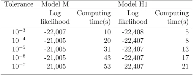
Table 3: Poisson log-likelihood and computing time in seconds for Models M and H1 for different tolerance levels in the one-stage approach with the approximate identifiability constrain
Tolerance Model M Model H1
Log Computing Log Computing
likelihood time(s) likelihood time(s)
10−3 -22,007 10 -22,408 5
10−4 -21,005 20 -22,407 8
10−5 -21,005 31 -22,407 13
10−6 -21,005 43 -22,407 17
10−7 -21,005 53 -22,407 21
Thus, the computing time has been speeded up, whereas the fit is just slightly worse. However, although the convergence problem seems to be solved for both Models M and H1, this cannot be said about the robustness issue. Model M is still quite unstable with regard to changes of in the data in both the age and period dimension. Model H1, being more simplistic, was already quite robust, and this has not changed by the added con-straint as well.
An important note I like to add is that one cannot blindly included the constraint. In essence, one is trying to fix certain characteristics of the global structure of the data, which differs between datasets. For the Hunt and Villegas constraint, it is shown by the authors of the paper themselves, the results are not universal for all datasets.
9
Hunt and Villegas (2015): Tests on Other Datasets
In other studies, similar problems with robustness and convergence in the one-stage fitting approach have been noted. These include:
• Data for the USA (Cairns et al. (2009) and Currie (2016))
• Data for Netherlands (van Berkum et al., forthcoming)
• Data for Spain (Deb´on et al. (2010))
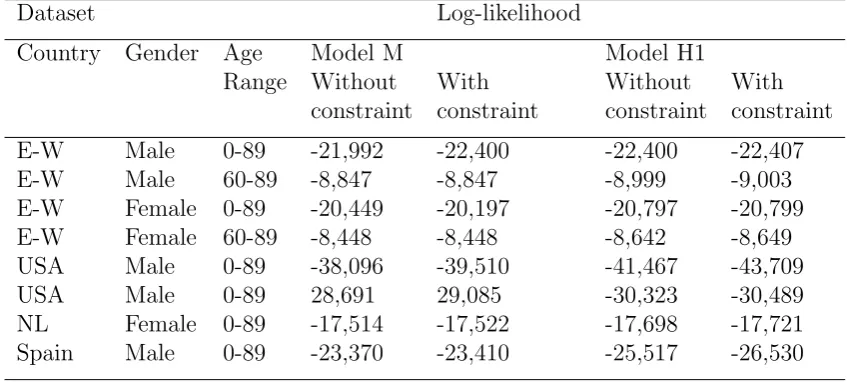
Table 4: Poisson log-likelihood for Models M and H1 in the one-stage approach with and without the approximate identifiability constraint
Dataset Log-likelihood
Country Gender Age Model M Model H1
Range Without With Without With
constraint constraint constraint constraint
E-W Male 0-89 -21,992 -22,400 -22,400 -22,407
E-W Male 60-89 -8,847 -8,847 -8,999 -9,003
E-W Female 0-89 -20,449 -20,197 -20,797 -20,799
E-W Female 60-89 -8,448 -8,448 -8,642 -8,649
USA Male 0-89 -38,096 -39,510 -41,467 -43,709
USA Male 0-89 28,691 29,085 -30,323 -30,489
NL Female 0-89 -17,514 -17,522 -17,698 -17,721
Spain Male 0-89 -23,370 -23,410 -25,517 -26,530
In Hunt and Villegas (2015) the authors note the other data-sets show many of the same issues with robustness and stability as those in the data for England and Wales Males in models M and H1. The use of the additional constraint partially resolves these issues, especially when using the H1 model. Thus these results are, therefore, strongly indicative that the issues and solutions are general features of models M and H1 and are not just specific to a single data set. However, it should also be noted that the difference in fit due to the additional constraint in the USA data is more significant, indicating that the values of the fitted κt are less linear compared to the other models. As such, one
should handle this with care.
10
Replicating the Tests
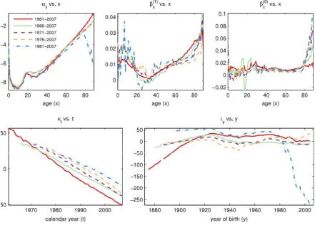
As described in Currie (2016), one can use the GNM (Generalized Nonlinear Models) R-package to fit the data. The GNM package is more detailed described in Turner and Firth (2007). This is utilized in the R-package StMoMo (stochastic mortality models) as described in Villegas et al. (2015). In order to effectively use StMoMo with the ap-proximate additional constraint as described earlier, one has to make certain adjustments in a few functions of both the StMoMo and the GNM package, as StMoMo uses GNM implicitly. Using this I made an attempt to replicate the results. As such, I tried to stay as close to the original code as possible, only adding the constraint and altering the code on places that disallowed the use of approximate transformations to the original fit-ted values. Yet, I obtained slightly different results compared to Hunt and Villegas (2015).
I tried to fit models M, H1 and APC to the data for three slightly different data-sets2:
• England and Wales Male data, age 0-89, years 1961-2007
• England and Wales Male data, age 0-89, years 1971-2007
• England and Wales Male data, age 0-89, years 1981-2007
10.1
Model M
Without the additional constraint, the dataset for years 1971-2007 fails completely3. By adding the constraint, the set behaves better, but is still way of the other parameter values. Even more interesting, the values of the κt, which are used for times series
forecasting in Lee and Carter (1992) show different slopes both with and without a constraint, as such, it seems to be meaningless to use them. In general, model M seems to be lacking robustness to be of any use, whatsoever.
10.2
Model H1
Model H1 seems to show more robustness, with regard to the fitting procedure, but it also obtains different values for the parameters. As such, it is not robust with respect to the parameters, however, it seems to be more robust compared to model M.
10.3
Convergence
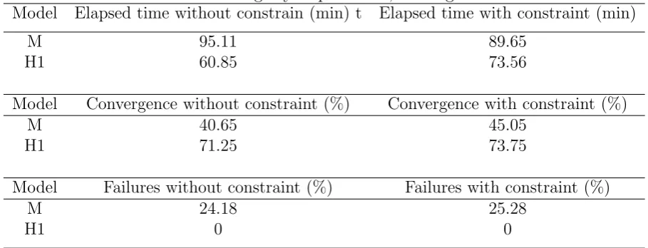
By subsetting the data based on the age in subsets for age 0-i, ∀i ∈ [10,89], one can assess roughly the time that would be saved by using the additional constraint. Whereas Hunt and Villegas (2015) finds performance increase, my findings are more modest, table 5.
Table 5: Overview findings by elapsed time, convergence and failures
Model Elapsed time without constrain (min) t Elapsed time with constraint (min)
M 95.11 89.65
H1 60.85 73.56
Model Convergence without constraint (%) Convergence with constraint (%)
M 40.65 45.05
H1 71.25 73.75
Model Failures without constraint (%) Failures with constraint (%)
M 24.18 25.28
H1 0 0
So, although the constraint seems to speed up model M slightly and solves the conver-gence problem partially, it does so for a price: e.g. the chance of a failure is higher, which makes sense as one uses an approximate transformation. Unwanted conditions during the iterative optimization could potentially be very harmful and lead to unexpected outcomes in terms of parameters. For model H1, it should be clear that the extra costs in time do not weigh against the slight benefit in terms of convergence.
All in all, I have to conclude from my results that the usage of the additional constraint is not beneficial to fitting the model. Even more so, it seems that the usage of model M and model H1, in terms of this data-set, should be avoided.
11
Conclusions
Compared to the conclusions drawn in the previous section, the authors of Hunt and Vil-legas (2015) draw different conclusions. They agree that the one-stage fitting procedure has considerable covergence and robustness problems, making the model sensitive to both the details of the fitting algorithm, the convergence criteria and the data the model is fitted to. They also find that model H1 is both more robust and achieves convergence more quickly. Also it is concluded that the addition of the extra constrain solves some of the robustness issues, but does not still not stabilize the model. A reason might be the fact that it is difficult to allocate structure in the data and assess the interactions between the variables. In conclusion, they argue for the use of model H1 in combi-nation with the additional constraint, based on theoretical justification and improved fit to data of the one stage-procedure, as has been argued in Cairns et al. (2009). This also improves the robustness of the model with respect to changes in the underlying data.
As such, I arrive at different conclusions, while using the same data and R-package, assuming Hunt and Villegas (2015) use StMoMo and GNM as well. The results I have obtained compel me to conclude that both model M and model H1 have serious disadvan-tages with respect to robustness and convergence. To obtain credible forecasts, neither model M nor H1 are supposedly to be used.
However, as stated in Beutner et al. (2016) the problem might be in the number of con-straints and the number of parameters. For example, in the appendix4, one can find
a section with graphs for the APC-model. These graphs show more robustness, while the model only contains three parameters and no multiplicative elements. Therefore, for modeling cohort effects this would be more suitable. For modeling with H1 or M, one should perhaps consider thus more constraints and even different constraints because the two constraints consideringι:
P
ιy = 0
P
(y−y¯)ιy = 0
in combination with the result that κt tends to be linear, might be problematic. As the
other elements in the model αx, β
(0)
x and βx(1) are fixed over time, changes of mortality
rates over time are explained by ιy and κt. Then imposing the above restriction on ιy
causes ιy to be either random around the ι = 0-line or causes all ιy to be zero. If you
apply the algorithm described in Hunt and Villegas (2015), you find that this particular combination of constraints may cause the loglikelihood value to become negative infinity and thus failing in general. Empirically, this is thus problematic.
The exact underlying mechanism is complex and more research should be focused on the underlying dynamics due to the constraints. Also, more attention should be paid to the nature of the data. Quite frankly, it is unwanted to assume certain model- and constraint-structures without a thorough analysis of the analytical goals and the underlying data.
References
Alho, J. M. (1990). Stochastic methods in population forecasting. International Journal of forecasting, 6(4):521–530.
Alho, J. M. (2000). the lee-carter method for forecasting mortality, with various exten-sions and applications , ronald lee, january 2000. North American Actuarial Journal, 4(1):91–93.
Beutner, E., Reese, S., and Urbain, J. (2016). Non-identifiability of popular extensions of the lee-carter model and plug-in lee-carter models.
Brillinger, D. R. (1986). A biometrics invited paper with discussion: the natural vari-ability of vital rates and associated statistics. Biometrics, pages 693–734.
Brouhns, N., Denuit, M., and Vermunt, J. K. (2002). A poisson log-bilinear regression approach to the construction of projected lifetables. Insurance: Mathematics and Eco-nomics, 31(3):373–393.
Cairns, A. J., Blake, D., Dowd, K., Coughlan, G. D., Epstein, D., Ong, A., and Balevich, I. (2009). A quantitative comparison of stochastic mortality models using data from england and wales and the united states. North American Actuarial Journal, 13(1):1– 35.
Currie, I. D. (2016). On fitting generalized linear and non-linear models of mortality. Scandinavian Actuarial Journal, 2016(4):356–383.
de Le´on, C. J. G. (1990). Empirical EDA Models to Fit and Project Time Series of Age-specific Mortality Rates: Y Jos´e G´omez de Le´on C. Central Bureau of Statistics.
Deb´on, A., Mart´ınez-Ruiz, F., and Montes, F. (2010). A geostatistical approach for dy-namic life tables: The effect of mortality on remaining lifetime and annuities.Insurance: Mathematics and Economics, 47(3):327–336.
Dowd, K., Cairns, A. J., Blake, D., Coughlan, G. D., Epstein, D., and Khalaf-Allah, M. (2010). Backtesting stochastic mortality models: an ex post evaluation of multiperiod-ahead density forecasts. North American Actuarial Journal, 14(3):281–298.
Good, I. J. (1969). Some applications of the singular decomposition of a matrix. Tech-nometrics, 11(4):823–831.
Goodman, L. A. (1979). Simple models for the analysis of association in cross-classifications having ordered categories. Journal of the American Statistical Asso-ciation, 74(367):537–552.
Hunt, A. and Villegas, A. M. (2015). Robustness and convergence in the lee–carter model with cohort effects. Insurance: Mathematics and Economics, 64:186–202.
James, I. R. and Segal, M. R. (1982). On a method of mortality analysis incorporating age-year interaction, with application to prostate cancer mortality. Biometrics, pages 433–443.
Keyfitz, N. (1982). Can knowledge improve forecasts? Population and Development Review, pages 729–751.
Kurzweil, R. and Grossman, T. (2005). Fantastic voyage: live long enough to live forever. Rodale.
Lee, R. D. and Carter, L. R. (1992). Modeling and forecasting us mortality. Journal of the American statistical association, 87(419):659–671.
Lov´asz, E. (2011). Analysis of finnish and swedish mortality data with stochastic mor-tality models. European Actuarial Journal, 1(2):259–289.
Renshaw, A. and Haberman, S. (2005). Mortality reduction factors incorporating cohort effects. Actuarial Research Paper (Cass Business School), (160).
Renshaw, A. E. and Haberman, S. (2003). Lee–carter mortality forecasting with age-specific enhancement. Insurance: Mathematics and Economics, 33(2):255–272.
Renshaw, A. E. and Haberman, S. (2006). A cohort-based extension to the lee– carter model for mortality reduction factors. Insurance: Mathematics and Economics, 38(3):556–570.
Sandberg, A. and Bostrom, N. (2008). Global catastrophic risks survey. civil wars, 98(30):4.
Thompson, W. S., Whelpton, P. K., et al. (1933). Population trends in the united states.
Tuljapurkar, S. and Boe, C. (1998). Mortality change and forecasting: how much and how little do we know? North American Actuarial Journal, 2(4):13–47.
Turner, H. and Firth, D. (2007). Generalized nonlinear models in r: An overview of the gnm package.
Villegas, A. M., Kaishev, V. K., and Millossovich, P. (2015). Stmomo: An r package for stochastic mortality modelling. In7th Australasian Actuarial Education and Research Symposium.
Whelpton, P. (1936). An empirical method of calculating future population. Journal of the American Statistical Association, 31(195):457–473.
Whelpton, P. K. (1928). Population of the united states, 1925 to 1975. American Journal of Sociology, pages 253–270.
Whelpton, P. K., Eldridge, H. T., Seigel, J. S., Siegel, J. S., et al. (1947). Forecasts of the Population of the United States, 1945-1975. US Govt. Print. Off.
Willets, R. (2004). The cohort effect: insights and explanations. Cambridge Univ Press.