Microstructure, renormalization, and more efficient vortex methods

Microstructure, Renormalization,

and More Ecient Vortex Methods

Alexandre J. Chorin

Department of Mathematics

University of California

Berkeley, California 94720-3840, USA

Abstract

The small-scale structure of the ow produced by vortex methods is discussed, and contrasted with the small-scale structure produced by grid methods. Particular attention is paid to the proliferation of vortex hairpins in three dimensions its origin is analyzed, a statistical description is given, and methods for harmlessly deleting unneeded hairpins are suggested. These methods involve renormalization-group ideas and an expansion in powers of a vortex fugacity. In both theory and applications, magnet variables play a major role.

1 Introduction

It is well known that the small-scale structure of the ows produced by vortex methods can dier substantially from the small-scale structure produced by other methods, even when large-scale features of the ow are very similar. Here are some examples: Boundary layers produced by vortex methods tend to be more oscillatory than their grid counterparts 15] in some circumstances, a vortex patch described by contour dynamics laments in a complex way 26], while a nite-dierence solution of the same problem is hard put to see any of the details of the lamentation even with heroic mesh renement 47]. Most troublesome, three-dimensional vortex lament or segment methods produce a proliferation of small-scale folds or \hairpins", which can make calculations expensive and inaccurate 12].

It is a small consolation that the microstructure produced by vortex methods is qualitatively correct, and indeed does lead one to reconsider the mathematical properties of the zero-viscosity limit of the Navier-Stokes equations and the basic assumptions of turbulence theory. Real ows do tend to \curdle" and produce intense vortex patches in two dimensions 45] and intense con-centrations in three 13]{ this is indeed the origin of intermittency a simple description in terms of vortices is attractive and also possibly misleading. One should make a sharp distinction be-tween modeling with vortices, in which one tries to get qualitative understanding with the help of a moderate number of vortices, and vortex methods as numerical methods, which stand or fall on their error bounds. Modeling and approximation should not be confused. They have separate roles if they are combined this must be done knowingly and carefully. For example, in two-space dimensions, vortex cores derived from physical analogies 10] deliver less accuracy than vortex cores obtained by approximation theory 5, 29]. Recent high-accuracy nite-dierence solutions of cav-ity problems 27] exhibit structures that are a vortex fan's delight, and can be readily modeled

Work supported in part by the Applied Mathematical Sciences subprogram of the Oce of Energy Research, U.S.

qualitatively by a small number of vortices and vortex dipoles these results are also expensive to reproduce accurately with a vortex method. The elaborate microstructure of vortex methods can be a boon to modelling and a heavy burden for approximation.

The advantages of vortex methods are low numerical viscosity, natural adaptivity, ease in inter-pretation and ease in imposing certain boundary conditions. The disadvantages are often related to the complex microstructure whether the price is worth paying depends on the problem, in par-ticular on the Reynolds number and on the accuracy desired. The solution of many problems is made easier if a good way to remove unwanted microstructure can be found.

2 An example of microstructure control

The complexity of small-scale vortex structure in three-dimensional vortex methods has been ob-served by many 49]. Numerical vortex laments can fold and stretch so that the task of following them becomes intractable. Smoothing of various kinds can delay this phenomenon, but then the eect of smoothing on accuracy must be weighed. Similar phenomena can occur at the boundaries of constant- vorticity patches in two dimensions, for which a control strategy has already been oered 25].

Folding in three dimensions starts for an obvious reason: one replaces a continuum distribution of vorticity by a bunch of laments (for the sake of brevity, the possibility of using segments, arrows, loops will not be mentioned explicitly). Vortex laments are unstable to perturbations whose wavelength is comparable to the vortex core 13, 53]. The evolution of the unstable modes generates spatial chaos, familiar from physical vortex systems such as fractal superuid vortices 2, 23], vortex glass phases in superconductors 32], and vortex lines in turbulence 13]. Indeed, the eort to understand numerical vortex folding has been useful in the analysis of these physical problems. However, numerical vortex folding is merely analogous, not identical, to physical vortex folding. The proliferation of numerical vortex elements is due in large part to numerical eects: Numerical instability, loss of accuracy and loss of resolution. Physical analogies are helpful heuristically, but must be used with great caution. In particular, as the numerical laments lengthen and their curvature grows (as it must, if only because the laments are typically conned to a nite volume), more integration points and shorter time steps should be used. If this is not done (and usually it cannot be done), the process of stretching and folding accelerates. Overproduction of vorticity marks underresolution (under other circumstances as well, see 6]). Soon the complexity of the ow and the attendant errors become overwhelming.

We shall try to gure out analytically the asymptotic behavior that the numerical vortex la-ments would have exhibited if only they had been calculated with no numerical error, and impose that behavior on the computed vortex system through renormalization. The original sin of replacing a continuum by a bunch of discrete objects is not erased discretization error, stability and moment errors 5] remain but are, one hopes, dramatically reduced. One would have liked to impose on the laments the asymptotic behavior of solutions of the Navier-Stokes or Euler equations, but it is not yet known how to do that. The assumption here is that the approximating vortex system would produce a good approximation if only its behavior in time were followed accurately.

that resembles in some ways the \surgery" introduced by Dritschel 25] in contour dynamics to reduce the complexity of stretching contours in the plane. There is a dierence in the details of the implementation between the two-dimensional and the three-dimensional cases, partly due to the fact that two-dimensional contours are smooth while vortex lines in three dimensions are not. More important, the theory that follows here is applicable so far only to three-dimensional ows. The key to the analysis is the observation that the stable equilibria of classical vortex systems lie on a phase transition line.

The paper is structured as follows: In Sections 3 and 4 we describe the stable equilibria of vortex laments in three dimensions, with some comments on irreversibility. In Section 4 we describe the uses of this theory, and in particular a renormalization procedure that simplies calculations without sacricing the asymptotic properties of vortex equilibria. In Section 5 we explain new techniques for satisfying boundary conditions in three-dimensional ows, needed for the application of our procedures they are discussed in detail elsewhere in this conference 52]. Some speculations and open questions are presented in the concluding section.

3 Statistics of a single vortex lament

We begin by considering the equilibrium statistical mechanics of a single vortex lament. This is already a non-trivial system because a single lament has a large number of degrees of freedom. The construction in this section is amply described elsewhere, see e.g. 13, 15]. Consider a single long vortex lament, with some small, nite, constant cross-section. Note that already here we depart from real uid mechanics and are considering the equilibrium statistics of a computational element a real vortex in a classical uid has a non-constant cross-section (indeed, probably a log-normal distribution of cross-sections 13]). It is immaterial for the analysis here whether the lament is open (a topological cylinder) or closed (a topological doughnut). The energy of a compactly-supported vorticity eld

=

(

x

) is given by the integral

E

_{= 18}

Z

d

x

Z

d

x

0

(

x

)

(

x

0) j

x

;

x

0 j

(1)

wherej

x

jis the length of the vector

x

. To specialize this integral to the case of a lament, suppose

the lament center-line can be approximately mapped on a connected set of

N

bonds of a cubic lattice then

E

is approximated by

E

N = X

i X

j6=i

t

i

t

j j

i

;

j

j

+

N

(2)

where

t

i is a vector centered at the center of the lattice bond occupied by the

i

-th piece of the

lament, parallel to that bond, pointing in the same direction as

in the bond, with j

t

i

j=

circu-lation of the vortex multiplied by the bond length and divided by p

8

,j

i

;

j

j is the straight-line

distance between segments

i

and

j

, and

is that portion of the integral in (2) which corresponds to

x,x

0 in the same bond. The parameter

will play an important role in the next section it

can be thought of as the energy per unit length of the vortex, if long range vortex interactions are neglected, and it is the analog of the \chemical potential" of statistical physics. We shall see that

controls the density of vortex laments. The device of attaching the vortex to a lattice is convenient, and produces very little loss in generality. The lament has many congurations. Assign to each conguration the \Gibbs" probability

Z

;1exp(

;

E

N), where

Z

is the appropriate

normalization factor,

E

N is the energy of the conguration,

= 1

=T

, and

T

is the \temperature".

temperature is discussed at length elsewhere 13]. The assumed probability distribution expresses thermal equilibrium. As in two space dimensions,

T

can be positive or negative

T <

0 is \beyond innity" rather than below 0 negative temperatures occur whenever the maxima of the entropy and of the energy fail to coincide. If the notion of negative temperatures is not comfortable, view it as a temporary aberration by the time we come to a many-lament system the range

T <

0 will become less important. If this \Gibbsian" probability distribution is assumed, then in the limit

N

!1, the vortex lament is in one of three states: For

>

0 it is balled up into a crumpled ball,

for

<

0 it is a straight line. The heuristics of this situation are simple:

>

0 favors (=assigns high probability to) low energy states, and low energy for a vortex is obtained by folding it and allowing the velocity elds induced by its several pieces to cancel the converse holds for

<

0. It is the boundary between these cases that is most important: When

= 0 all the exponents in the Gibbs distribution are zero, and all congurations are equally likely. In addition, congurations with two pieces of the vortex occupying the same lattice bonds are forbidden, by conservation of volume. A collection of congurations of a lattice vortex, all equally likely, with no overlaps, is known as a \polymer", because it is often used as a model for a polymer in a solution. A lot is known about this kind of polymers, in particular from long experience with numerical computation 28]. A typical polymer is non-smooth, and has fractal dimension

D

= 1

:

70

:::

. The quantity 1

=D

is known as the \Flory exponent". If the vorticity has support on a \polymer", its energy spectrum has a power law 13, 57].

This picture does not change if we replace a single lament by an innite collection of laments, as long as they are far enough from each other so as not to feel each other's presence. The limit

N

! 1 for each of these laments can be reached by reducing the length of the bonds in the

lattice.

We now claim that it is the \polymeric"

= 0 state that is important in uid mechanics because it attracts other equilibrium states i.e., even if one starts with

6= 0, one ends up with

= 0, as the result of vortex stretching. Indeed, consider a smooth physical vortex with some nite cross-section. It can be modeled as a nite collection of segments, at a negative

(or else the lament is too crumpled to model something smooth). If the vortex is imbedded in a random ow it will presumably stretch 13, 21] if its energy is conserved one can see that j

jwill decrease until

= 0 is reached, assuming the evolution can be modelled as a succession of equilibrium states. The heuristics here too are straightforward: Vortex stretching creates new bonds without adding energy the energy per bond decreases, reducing the temperature. Energy conservation forbids the crossing of the boundary

= 0 (see more below), which is therefore attracting. We thus have a simple near-equilibrium cartoon of the eect of vortex stretching and of the reason for the appearance of a Kolmogorov spectrum. In two space dimensions, by contrast, there is no stretching, the temperature of a vortex system is invariant (assuming adiabatic walls), and there is no universal spectrum. The conclusion is that a very sparse collection of thin vortex laments will end up having an innite temperature, with each vortex lament having a fractal centerline. The constant

plays a secondary role further analysis shows that it plays a role in creating intermittency, which does not concern us here.

4 A collection of vortex laments

of this line (which includes the half plane

<

0, since negative temperatures are \hotter" than positive temperatures), and vortex stretching draws them to the transition line. Note that the numerical vortex lines have a constant cross-section, like some models of superuid vortex lines but unlike physical vortices. This emphasizes again that a physical vortex line must be approximated by a cloud of numerical vortex lines.

To understand the situation analytically, we proceed via a Kosterlitz-Thouless (KT) \dielectric" analysis 36, 37], which is a two-term expansion in powers of the fugacity

y

=

e

;, and applies

to sparse (but no longer one-lament) systems. The analysis of the previous section will turn out to be the

y

! 0 limit of this theory. The \dielectric" formalism is not uniquely dened 19], and

will will pick its easiest version 18]. The formalism has the great advantage of leading naturally to irreversible extensions of the equilibrium theory.

First, following 43, 54] we simplify the vorticity eld and represent it as a sparse collection of planar, circular vortex loops. Recent work, in particular by Buttke 7, 8], shows that any vorticity eld can be approximated by a union of circular loops (also known as \magnets", or \elements of impulse" or \velicity") indeed, every closed vortex lament can be decomposed into small planar loops: Simply span the lament by a surface, and break the surface into small pieces assign to each piece a vortex loop with the same circulation as the original closed vortex lament, and spanning an area equal to the area of the small piece. This representation is not unique, as is obvious from the non-uniqueness of the spanning surface, and this creates problems when entropy is calculated furthermore, the surface elements on the surface must coalesce into a coherent surface, and are not free to rotate as will be assumed in the argument that follows now. The loop representation thus constitutes a substantative simplication 14], and we shall not dwell on the errors that it produces. One can attach to each small planar loop (or \magnet", so called by analogy with magnetostatics) an arrow perpendicular to its plane and oriented by the direction of the vorticity in the loop such an oriented magnet will be denoted in this section by

m

.

Suppose for a moment that the temperature

T

of the system of vortex loops is small, and accept the idea that the temperature dened above as a parameter in a Gibbs distribution does indeed correspond to what is usually thought of as temperature. If

T

is positive and very small, there will be very few loops in the system and the impulse they carry will be small. The impulse of a vortex loop is the integral 1

2

R

l oop

x

d

s

, where

is the circulation in the loop and

d

s

is an

element of arc length if the loop is planar, the impulse reduces to

A

, where

A

is the area spanned by the loop 13, 33]. As the temperature increases, there will be more loops and larger loops. As long as the loops are small and disconnected, the loop representation presents no problems the loops are independent and their spanning surfaces can be easily chosen by a common convention (for example, as the minimal surfaces attached to each loop for a detailed analysis, see 23]). The growth in the number of loops and in the size of the loops are related: If one takes a large loop and places inside it a smaller loop with opposite orientation, the energy of the combined conguration is reduced and its appearance is more likely (this is "polarization") thus a cloud of small loops allows large loops to form. Eventually, it becomes possible for an innite loop to form. The result is a percolation threshold and a phase transition in the vortex system 1, 13]. In the theory of superuids, this phase transition corresponds to the transition from a superuid to a normal uid we shall argue below that this is also the attracting equilibrium for a classical uid (i.e., for the set of "excitations", or modes of motion, that make up turbulence is the usual type of uid).

Suppose a velocity

u

is imposed on the cloud of vortex loops. The loops will orient themselves so as to oppose that velocity. The reduction in energy due to the presence of a magnet

m

is

1 2

m

u

. The average polarizability of the loop, i.e., the average value of

m

u

divided by

u

=j

u

j

is 1 12

m

2, where

m

=

j

m

j. This calculation can be found e.g in 18]: One averages over all solid

angles, weighing each by the appropriate Gibbs factor which favors lower energies. We already know that

m

=

r

2, where

r

is the radius of the loop thus polarizability is a function of

r

.

Next one has to nd the density of loops of radius r. We view the number of loops as variable, and thus it is the grand-canonical ensemble that is relevant. In order to use this ensemble in a classical uid mechanical context, where loops cannot be created by thermal uctuations because of the conservation of circulation and can only be created by vortex stretching and reconnection, one has to invoke a generalized ergodic principle 40] to the eect that thermal equilibrium will not be denied regardless of the precise mechanics involved.

The grand-canonical partition function is an expansion in powers of the fugacity

y

= exp(;

loop), where

loop is the energy needed to create a single loop of radius

r

. For an isolated circular

loop this energy equals

r

log

r

, where

, the energy per unit length of the vortex loop, is closely related to the

of Eq. 2 above. The coecient of

y

is the partition function for a one-loop system, the sum of possible states of that system per unit volume times their Gibbsian weights 31]. If the fugacity is small enough one can be content with this single term which is then the density of the the loops of radius

r

. (Note that the zero-order term in

y

does not contribute to the polarization). To enumerate all states one needs an estimate of the smallest length scale in the problem. For a collection of thin circular laments it is natural to take the small diameter

of the laments as this smallest length scale. In a unit cube there are

;3 possible loop centers. All orientations of the

loops are possible, albeit with dierent probabilities There are 4

r

2

dr

;3 distinct orientations of

a loop with radius between

r

and

r

+

dr

. Each of these has to be multiplied by the corresponding Gibbs factor exp(;

E=e

), where

E

is the energy of interaction between the loop under discussion

and all the others, and

e

=

e

(

r

) is the dielectric \constant", which, in the absence of a scale separation between large and small loops, may well be a function of

r

. In fact, one must gure out how a loop of radius

r

is formed and write a history-dependent expression for the potential in the Gibbs factor, see 19], but we shall not need this degree of renement: In a low-fugacity system,

E

is negligible. The dielectric constant is the sum of all these contributions as

r

ranges from

to innity. It is customary to introduce the function

K

=

K

(

r

) by

e

(

r

) =

=K

(

r

). Note that the unknown

e

or

K

appears in the exponential. We shall assume for simplicity that

K

is in fact a constant the equation for

K

is nonlinear:

K

;1 =

;1+

c

1

Z 1

r

6exp( ;

Kc

2

r

log

r

))

dr

(3)

where the constant

c

1 can be evaluated from the preceding discussion, and is proportional to

;6.

(More precisely,

c

1= (4

=

3)

4

2

;6 the powers of

come about as follows: Two from the formula

for polarizability, one from the enumeration of states due the rotations of the loops, and one from the 4

in the relation between loops and the induced velocity 33].) The estimation of the parameter

c

2 involves some elaborate manipulations. The easiest way to nd it is as follows: Assume the

energy of a loop can be found as the product of an energy per unit length of the lament (dened in Eq. 2 with bond length 1) times the length this requires dropping log

r

from the denition of the energy of a loop|a small error (in 18] it is shown that this simplication is entirely legitimate for fractal loops, but we are not invoking a fractal loop model). Now we need only the energy per unit length of the numerical vortex. Suppose the vortex is approximated as a sum of blobs. Let

integration, one must carefully account for the assumed direction of the vorticity eld in the blob

Q

is an attribute of the numerical method, and remains xed as long as the same blob function is used. For the 4th-order Beale-Majda blob 5]

Q

= 5

:

17. A simple scaling analysis shows that if the blob radius is

rather than 1, the corresponding energy is

Q=

. The circulation

multiplies this energy by

2. If there are

M

= 1

=h

blobs per unit length of the vortex, where

h

is the inter-blob

distance, then

=

Q

2

=h

.

Equation 3 can now be rewritten in the form

T

=

;1 =

K

;1 ;

c

1 Z

1

d

r

6exp(

;

Kr

)

dr :

(4)

As was noted by Hald 30], the right-hand side of (5) is a convex function of

K

with a single maximum

T

0 at some

K

0. For

T > T

0 Eq. 5 cannot be satised with

K

real, and we are outside

the region of validity of the \dielectric" approximation, i.e., we have crossed the phase transition line. As

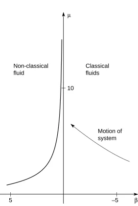
varies one obtains dierent values of

0= 1

=T

0 which trace out the phase transition line,

sketched for a particular choice of parameters in Fig. 1. Note that this graph is consistent with the single-lament model: As

!1the system becomes more sparse and the phase transition line is

asymptotic to the

= 0 axis, which was the result of the preceding section. Note that

K

changes across the phase transition line: We have

K >

1 to the left the integral equation yields a complex

K

on the right, but by then the model does not apply as it stands.

The discussion just given has heuristic elements and mathematical diculties 19]. Its great advantage is that one can imbed into the \dielectric function" formalism a non-instantaneous response of the loops to a variable imposed velocity, and as a result obtain a description of non-equilibrium phenomena \near" the non-equilibrium congurations we have just calculated 3, 16, 39]. This is an important point, in particular because it reconciles the \equilibrium" model with the irreversible aspects of turbulence, but it does not otherwise concern us here, see 16]. It is comforting that the results we have obtained agree reasonably well with numerical data 2, 35]. These results can also be derived by more sophisticated procedures, in particular by a perturbation expansion on the cold side of the transition and by hydrodynamic methods on the \hot" side these more elaborate constructions will be presented elsewhere.

Our assumption is that if an ensemble of numerical vortex laments is followed accurately, it will come to reside on the phase transition line. One expects the vortex centerlines to become fractal, as in the very sparse system of the previous section, and thus it is not expected that a straightforward numerical calculation will do a good job of following the collection to its resting place. However, the information available about the phase transition line can be put to good use and improve the numerical calculations, as shown in the next section.

5 Renormalization and hairpin removal

The dielectric formalism lends itself to a renormalization group analysis (see 19, 35]), of which we are now going to produce a simplied version. Dierent applications of renormalization groups in uid mechanics can be found can be found in 4, 41, 44, 56].

will be disregarded (and in particular, we shall pursue calculations over times so short that energy dissipation can be neglected), and we shall adhere to the constant

K

model used above, where

K

is a constant that satises a certain nonlinear equation. In a more general treatment, one has to allow

K

to vary with scale.

The typical vortex calculation is made in terms of vortex laments rather than vortex loops (the diculties in using loops are analyzed in detail in 23] one context in which loops are useful is near walls, see 22, 52] and below). We shall rst consider a hypothetical calculation that does use loops, and then translate the results to the language of laments.

Suppose you have a collection of vortex loops with inverse temperature

and chemical potential

, with values that correspond to the transition line. On the \cold" side of the line one has a dielectric constant

K

=

K

(

), which has been calculated at the same time as

, given

and the other constants: (

;1 is the maximum of the right-hand side of Eq. 4 reached at the appropriate

value of

K

=

K

0). On the \hot" (high

T

=

;1 side) the theory above is not dened complex

values of

T

are meaningless. To the extent that this theory can be taken seriously, one can think that it breaks down slowly (for example, as a result of a gradual build-up of large scale vortices, and that on the transition line

K

=

K

0, i.e., one can assume that the

K

from the left extends to

the boundary. This is not an obvious conclusion, and we expect to examine it carefully in later work. Notice in particular that in the previous section, as in other folding transitions 13], there are three distinct states, one on each side of the transition line and one on the line itself.

Assuming that

K

is known on the transition line, and that one has an equilibrium critical state, suppose that all loops of radius

r

d

are simply deleted from the calculation. The total

contribution to the dielectric constant of the loops deleted is

e

(

d

) =

=K

= 1 +

c

1 Z

d

r

6exp(

;

K

)

dr

= 1 +

C

(

d

)

(5)

and the remaining loops have interactions lowered by 1 +

C

(

d

). In an homogeneous medium all one has to do is reduce the strengths of all the vortices by this factor, 1 +

C

(

d

). Hopefully,

d

is large enough so that the motion of the remaining loops can be followed accurately, but not so large that the nite rate of relaxation of equilibrium of the loops of scale

d

cannot be neglected in what is only approximately an equilibrium theory. One can easily see that the larger the loop, the longer is the time it takes to relax to equilibrium indeed, if it is large enough it will never relax to equilibrium in the presence of external stirring. We have thus succeeded in imposing the correct asymptotic properties of the collection of vortex laments on the numerical calculation, leaving for direct computation a task that has become more aordable.

A special case that is particularly easy to deal with is the one of a very sparse collection of vortices. One can go through the formalism above and see that the renormalization parameter 1+

C

(

d

) is very close to 1 for a sparse collection. Indeed, for a sparse collection one should be able to use the one-vortex theory of the preceding section in which the critical line is

= 0. On that line, all the Gibbs factors are unity, there is no polarization, and small loops can be removed without penalty, as was indeed done in 12]. The enormous gain in computer eort and the negligible cost in accuracy are exhibited in that reference.

laments as an indicator of the scale of the appropriate smaller loops. There is no unique way of doing that. Experience seems to indicate that it is very dicult to recognize the scale of loops in calculations based on vortex elements which do not individually have zero divergence (for example, with vortex \arrows"). The issue is discussed in 12] and, with much more detail, in 20].

Another issue that will be addressed in 20] is the modication of the renormalization for inhomogeneous systems. To a rst approximation, when

C

(

d

) is small, the inhomogeneity can be ignored as was done in 12]. However, this is not a satisfactory general method. If one considers two patches of vorticity at some distance from each other, with no vorticity in between, the velocity eld due to one patch moves the second patch as a whole the polarization of loops inside a patch aects the velocity distribution within the patch but not the velocity of the patch. The issue that arises here is the issue of galilean invariance in hydrodynamics for an early seminal discussion see 38].

6 More on the magnet representation

As was already mentioned above, several authors 8, 42, 48, 50] have noted the possibility of writing the Euler and Navier-Stokes equations in three space dimensions in terms of \magnetization" (or \impulse", \velicity") Buttke 8],9] has constructed a numerical method based on this represen-tation coupled with a blob mollication this numerical method gives rise to a Hamiltonian system at each level of approximation. Cortez 22] has shown how to adapt the high-accuracy blobs of vortex theory to produce high-order accurate magnet approximations. It is shown in 22, 23] that the magnet representation in free space is not trouble-free: the amplitude of the computational elements is proportional to the area of certain \normal" surfaces, and can grow without bound even when the vorticity remains uniformly bounded. To run successfully, one has to introduce sophisticated remappings. However, near walls, magnets can be very useful, in particular because they allow the creation of vorticity at walls in three space dimensions in the form of closed loops, and thus make hairpin removal/renormalization much easier. The diculties one can encounter in creating loops by other means are described in 51].

To develop the magnet representation, start with the observation that the velocity

u

is the vector potential for the vorticity:

= curl

u

. In a simply connected domain the addition of grad

q

to

u

leaves

invariant (we consider only the three-dimensional case). Given an arbitrary

q

at

t

= 0, one can nd equations of motion for

m

=

u

+ grad

q

. In the Euler case (

R

= 1), if

m

= (

m

1

m

2

m

3),

u

= (

u

1

u

2

u

3), these equations are

Dm

i

Dt

@

t

m

i+

u

j

@

j

m

i= ;

m

j

@

i

u

j (6)

u

=P

m

(7)

where P is the Hodge projection that extracts from

m

its divergence-free part that is tangent to

the boundaries. (The addition of viscosity adds a term

R

;1

m

to (6), and requires a careful

consideration of boundary conditions, becausePand do not necessarily commute in the presence

of walls.) If the vorticity

has support in a nite ball

B

, it is possible to pick

q

so that at

t

= 0,

m

= 0 outside

B

, and then

m

retains a compact support for all

t >

0. This condition is however not sucient to x

m

uniquely. We shall henceforth assume that

m

has compact support if

does.

To construct a Lagrangian numerical method, write

m

=

m

(

x

t

) =P i

M

i(

t

)

(

x

;

x

from (6) one nds

d

(

M

i)k

dt

=;(

M

i)j

@

k

u

j(

x

i)

(8)

where (

M

i)k is the

k

-th component of

M

i in addition,

d

x

i

dt

=

u

(

x

i)

u

=

P

m

(9)

where the projection is to be performed on the function

m

dened by the magnetization blobs (= \magnets"). This is easily done: One can check that for all

t >

0, the

m

produced by Eq. (6) diers from

u

by a gradient

q

=

q

(

x

t

). Write

q

= !

q

i,

u

i

;

M

i

(

x

;

x

i) = grad

q

i hence

q

i= ;div(

M

) ( = Laplace operator) let

= ;1

, then

q

i = div(

M

i

(

x

;

x

i)) = (

M

i)k

@

k

,

(grad

q

i)k = (

M

i)`

@

`

@

k

, and (

u

i)k = (

M

i)k

;(

M

i)`

@

`

@

k

. Finally,

u

(

x

i) = P

j

u

j(

x

i) (the

velocity at a point is the sum of the velocities generated by all the loops).

One can readily verify that the system (8), (9) is Hamiltonian, with HamiltonianH= 1 2 P i

M

i

u

i. The variables (

M

i)

k

(

u

i)

k are conjugate. The vector

m

has velocity units, and the units of

M

are velocity volume. One can also check that the velocity eld

u

i due to the

i

-th magnet is

identical at large distances to the velocity eld due to a small, circular vortex loop (see e.g. 33]). Thus the \magnet" representation is a loop representation like the one we used for KT theory.

In vortex methods, the no-slip boundary condition is usually satised by creating vorticity. At each boundary point, the velocity defect can be readily found, and a vortex \arrow" created. Arrow representations require care under the best of circumstances 55], but are particularly awkward when one sets out to recognize and remove small loops (= hairpins). It is dicult to string the arrows into closed loops. The magnet representation neatly side-steps the problem.

The key observation is that force acting on a uid imparts impulse to the uid. Impulse is identical with magnetization. There are many ways of using this observation, corresponding to the multiple choices of gauge in the denition of

m

. One possibility is to start by creating vortex sheets at walls, calculate the impulse associated with them, and replace them at some point by loops of equal impulse. A complete construction is given in 52]. These loops are then fodder for hairpin removal.

7 Conclusions and warnings

We have produced a theory that leads to implementable algorithms for simplifying vortex calcula-tions and taming their microstructure. The idea that much of the microstructure is either unneeded or misleading is natural the theory has the added advantage of providing a systematic approxi-mation procedure which in principle can be used to gauge the reliability of the simplication. The theory, as presented here, rests in particular on the idea that if one could follow the approximate vortex representation accurately, one would obtain a good approximation to the Euler equations even for long times the truth of this idea is not self-evident, and it must be viewed as only a plausible guess.

At several places in the analysis various simplications were made, which must be examined in greater detail. The KT (Kosterlitz-Thouless) dielectric model is open to various challenges, and its continuation across a transition line requires a clearer analytical justication.

turbulence, and allow one also to decide whether vortex descriptions provide an adequate tool for describing turbulent ow. Adequate eld descriptions already exist for superuid vortices 34] the dierences between superuid vortices and classical vortices 7] are beginning to be well understood, and a eld-theoretical analysis of vortex interactions and their renormalization is within sight 13].

References

1] Akao, J., \Percolation in a Three-Dimensional Vortex Gas Model of the

Transition," submitted for publication, 1995.

2] Akao, J., \Phase Transitions and Connectivity in Three-Dimensional Vortex Equilibria," Ph.D. Thesis, Mathematics, Univ. of California at Berkeley, 1994.

3] Ambageokar, V., Halperin, B., Nelson, D. and Siggia, E., \Dissipation in Two-Dimensional Superuids," Phys. Rev. Lett.,

40

, pp. 783{786, 1978.

4] Avellaneda, M. and Majda, A., \Simple Examples with Features of Renormalization for Tur-bulent Transport," Phil. Trans. R. Soc. London A,

346

, pp. 205{233, 1994.

5] Beale, J.T. and Majda, A., \High Order Accurate Vortex Methods with Explicit Velocity Ker-nels," J. Comp. Phys.,

58

, pp. 188{208, 1985.

6] Brown, D. and Minion, M., \Performance of Underresolved Two-Dimensional Incompressible Flow Simulations," J. Comp. Phys., in press, 1995.

7] Buttke, T., \Numerical Study of Superuid Turbulence in the Self-Induction Approximation," J. Comp. Phys.,

76

, pp. 301{326, 1988.

8] Buttke, T., \Lagrangian Numerical Methods which Preserve the Hamiltonian Structure of In-compressible Fluid Flow," Vortex Flows and related Numerical Methods, edited by J.T. Beale, G.H. Cottet and S. Huberson, NATO ASI Series, vol.

395

, Kluwer, Norwell, 1993.

9] Buttke, T. and Chorin, A., \Turbulence Calculations in Magnetization Variables," Appl. Num. Math., bf 12, pp. 47{54, 1993.

10] Chorin, A.J., \Numerical Study of Slightly Viscous Flow," J. Fluid Mech.,

57

, pp. 785{796, 1973.

11] Chorin, A.J., \Hairpin Removal in Vortex Interactions," J. Comp. Phys.,

91

, pp. 1{21, 1990. 12] Chorin, A.J., \Hairpin Removal in Vortex Interactions II," J. Comp. Phys.,

107

, pp. 1{9, 1993. 13] Chorin, A.J., Vorticity and Turbulence, Springer, 1994.

14] Chorin, A.J., \Vortex Phase Transitions in 2.5 Dimensions," J. Stat. Phys.,

76

, pp. 835{856, 1994.

15] Chorin, A.J., \Vortex methods, Lectures at Les Houches Summer School of Theoretical Physics," 1993 (In press).

17] Chorin, A.J. and Gu, M., Turbulent Cascades Through Equilibrium Spectra, Manuscript, Univ. of California at Berkeley, Math. Dept, 1995.

18] Chorin, A.J. and Hald, O., \Vortex Renormalization in Three Space Dimensions," Phys. Rev. B,

51

, pp. 11969{11972, 1995.

19] Chorin, A.J. and Hald, O., Analysis of Kosterlitz|Thouless Transition Models, Manuscript, Univ. of California at Berkeley, Math Dept, 1995.

20] Chorin, A.J. and Knio, O., Renormalization of Vortex Calculations, in preparation.

21] Cocke, W.J., \Turbulent Hydrodynamic Line Stretching: Consequences of Isotropy," Phys. Flu-ids,

12

, pp. 2488{2492, 1969.

22] Cortez, R., \An Approximation of Fluid Motion due to Boundary Forces Using Impulse Vari-ables," in press, J. Comp. Phys., 1995.

23] Cortez, R., Impulse Based Methods for Fluid Flow, Ph.D. thesis, Mathematics, Univ. of Cali-fornia at Berkeley, 1995.

24] Donnelly, R.J., Quantized Vortices in Helium II, Cambridge Univ. Press, 1991. 25] Dritschel, D., \Contour Surgery," J. Comp. Phys.,

77

, pp. 240{266, 1988.

26] Dritschel, D., \The Repeated Filamentation of Two-Dimensional Vorticity Interfaces," J. Fluid Mech.,

194

, pp. 511{547, 1988.

27] E, W. and Liu, J.G., Essentially Compact Schemes for Unsteady Viscous Incompressible Flow, Manuscript, Institute for Advanced Study, Princeton, 1995.

28] Gennes, P.G. de, Scaling Concepts in Polymer Physics, Cornell Univ. Press, 1971.

29] Hald, O.H., \Convergence of Vortex Methods for Euler's Equations III," SIAM J. Num. Anal.,

24

, pp. 538{582, 1987.

30] Hald, O., Personal Communication.

31] Huang, K., Statistical Mechanics, Wiley, New York, 1963.

32] Huse, D., Fisher, M. and Fisher, D., \Are Superconductors Really Superconducting?", Nature,

358

, pp. 553{559, 1992.

33] Jackson, J.D., Classical Electrodynamics, Wiley, New York, 1974.

34] Kleinert, H., Gauge Fields in Condensed Matter, World Scientic, Singapore, 1989.

35] Kohring, G. and Shrock, R., \Properties of Generalized 3D

O

(2) Model with Suppression/ Enhancement of Vortex Strings," Nuclear Physics B,

288

, pp. 397{418, 1987.

36] Kosterlitz, J., \The Critical Properties of the Two-Dimensional

xy

Model," J. Phys. C: Solid State Phys.,

7

, pp. 1046{1060, 1974.

38] Kraichnan, R., \Lagrangian-History Closure Approximation for Turbulence," Phys. Fluids,

8

, pp. 575{598, 1965.

39] Landau, L. and Lifshitz, E., Statistical Physics, 3rd edition, part 1, Pergamon, New York, 1980. 40] Langer, J. and Reppy, J., \Intrinsic critical velocities in superuid helium," Progress in Low

Temperature Physics, vol. VI, edited by C. Gorter, North-Holland, Amsterdam, 1970. 41] Lesieur, M., Turbulence in Fluids, Kluwer, Dordrecht, 1990.

42] Luchini, P., \Magnetization Vector Analogy as a Reformulation of the Equations of Fluid Me-chanics," AIAA J.,

29

, pp. 474{477, 1991.

43] Lund, F., Reisenegger, A. and Utreras, C., \Critical Properties of a Dilute Gas of Vortex Rings in Three Dimensions and the

Transition in Liquid Helium," Phys. Rev. B,

41

, pp. 155{161, 1990.

44] McComb, W.D., Physical Theories of Turbulence, Cambridge Univ. Press, 1989.

45] McWilliams, J., \The Emergence of Isolated Coherent Vortices in Turbulent Flow," J. Fluid Mech.,

146

, pp. 21{46, 1984.

46] Meneveau, C., \Dual Spectra and Mixed Energy Cascade of Turbulence in the Wavelet Repre-sentation," Phys. Rev. Lett.,

66

, pp. 1450{1453, 1991.

47] Minion, M., Two Methods for the Study of Vortex Patch Evolution on Locally Rened Grids, PhD Thesis, Univ. of California at Berkeley, Math. Dept., 1994

48] Oseledets, V.I., \On a New Way of Writing the Navier-Stokes Equations: The Hamiltonian Formalism," Comm. Moscow Math. Soc. 1988, translated in Russ. Math. Surveys,

44

, pp. 210{ 211, 1989.

49] Puckett, E.G., \A Review of Vortex Methods," Incompressible Computational Fluid Mechanics, edited by R. Nicolaides and M. Ginzburger, Cambridge Univ. Press, 1992.

50] Rouhi, A., Poisson Brackets for Point Dipole Dynamics in Three Dimensions, Manuscript, Univ. of California at San Diego, 1990.

51] Summers, D., An Algorithm for Vortex Loop Generation, LBL report LBL-31367, Berkeley, Calif., 1991.

52] Summers, D. and Chorin, A.J., \Hybrid Vortex/Magnet Methods for Flow over a Solid Bound-ary," Vortex Flows and Related Numerical Methods II, edited by Y. Gagnon et al., ESAIM: Proc.,

1

, http://www.emath.fr/proc/Vol.1/, pp. 65{76, 1996.

53] Widnall, S., \The Structure and Dynamics of Vortex Filaments," Ann. Rev. Fluid Mech.,

8

, pp. 141{165, 1976.

54] Williams, G., \Vortex Ring Model of the Superuid

Transition," Phys. Rev. Lett.,

59

, pp. 1926{1929, 1987.

56] Yakhot, V. and Orszag, S., \Renormalization Group Analysis of Turbulence I: Basic Theory," J. Sci. Comp.,

1

, pp. 3{51, 1986.

57] Zeitak, R., Vectorial Correlations on Fractals: Applications to Random Walks and Turbulence, Manuscript, Weizmann Institute of Science, 1992.

Motion of system Non-classical

fluid

Classical fluids 10

5 –5 β

µ

XBD 9506-03028.ILR