© Shiraz University
A GENERALIZED KERNEL-BASED RANDOM K-SAMPLESETS
METHOD FOR TRANSFER LEARNING
*J. TAHMORESNEZHAD AND S. HASHEMI
**Electrical and Computer Engineering School, Shiraz University, Shiraz, I. R. of Iran Email: [email protected]
Abstract– Transfer learning allows the knowledge transference from the source (training dataset) to target (test dataset) domain. Feature selection for transfer learning (f-MMD) is a simple and effective transfer learning method, which tackles the domain shift problem. f-MMD has good performance on small-sized datasets, but it suffers from two major issues: i) computational efficiency and predictive performance of f-MMD is challenged by the application domains with large number of examples and features, and ii) f-MMD considers the domain shift problem in fully unsupervised manner. In this paper, we propose a new approach to break down the large initial set of samples into a number of small-sized random subsets, called samplesets. Moreover, we present a feature weighting and instance clustering approach, which categorizes the original feature samplesets into the variant and invariant features. In domain shift problem, invariant features have a vital role in transferring knowledge across domains. The proposed method is called RAkET (RAndom k samplesETs), where k is a parameter that determines the size of the samplesets. Empirical evidence indicates that RAkET manages to improve substantially over f-MMD, especially in domains with large number of features and examples. We evaluate RAkET against other well-known transfer learning methods on synthetic and real world datasets.
Keywords– Transfer learning, unsupervised domain adaptation, random samplesets, feature weighting, instance clustering
1. INTRODUCTION
The main assumption of learning algorithms is that the data used for training and testing are drawn from the same distribution. However, this assumption is challenged in many real world applications [1]. In some special cases like spam detection, where data is easily outdated, the training and testing data obey different distributions. As another case, in machine translation [2] and sentiment classification problems [3], we might want to adapt a learning algorithm trained on some products for a new product that helps to reduce the effort of annotating reviews for new products. However, the reviews may be different for various products and training and testing data have different distributions.
In general, domain adaptation approaches are divided into two settings: unsupervised domain adaptation where the target domain is fully unlabeled, and semi-supervised domain adaptation where the target domain contains a small amount of labeled data. This paper focuses on the feature selection for transfer learning (f-MMD) [4], which is an unsupervised domain adaptation method. f-MMD is an interesting approach to study, as it has the advantage of transfer learning in the original feature space. f-MMD tries to learn some domain invariant features across domains in a Reproducing Kernel Hilbert Space (RKHS) using maximum mean discrepancy (MMD) [5].
However, f-MMD is challenged in domains with large number of features and training examples due to the typically proportionally large number of variables appearing in the optimization problem. The
Received by the editors December 31, 2014; Accepted May 25, 2015.
number of variables raises the computational cost of f-MMD on one hand, and makes it quite unsolvable in some datasets with a few more features or instances on the other hand. Moreover, f-MMD learns invariant features fully unsupervised and dismisses the relation of features to class labels. Nevertheless, some of the removed variant features have strong relations to the class labels and influence the classifier performance.
In order to deal with the aforementioned problems, this work proposes randomly breaking the initial set of samples into a number of small-sized samplesets, and employing kernel based feature weighting approach to learn invariant features of domains. Our main contributions are as follows: i) a new perspective to divide large datasets to small-sized random samplesets, ii) a kernel based feature weighting and instance clustering approach, and iii) a new representation for dataset in its original feature space. The proposed method is called RAkET (RAndom k samplesETs), where k is a parameter that specifies the size of the samplesets.
The rest of this paper is organized as follows. We briefly review the related work in the next section. Then the theoretical background behind of the proposed approach is described in Section 3. Section 4 introduces the proposed method and presents the main algorithm. We evaluate our method on a variety of datasets with different number of features, instances and distributions in Section 5. This will be followed by the conclusion and future work in the last section.
2. RELATED WORK
In unsupervised domain adaptation, there are generally three types of approaches: i) common feature representation, ii) weighting individual instances, and iii) weighting individual features. The first group learns a domain invariant representation on which the distribution of source and target domains are closer than under the ambient feature space [6-11]. The main drawback of these methods is that the joint optimization of predictor and representation is difficult and prevents them from focusing on predictive features.
The second group endeavors to minimize the difference between domains, typically by weighting the individual instances [12, 13]. In some proposed methods [14, 15], MMD of the source and target domains is used for reweighting of the examples. Gong et al., 2013, proposed a novel approach for selecting the landmarks among the source examples based on MMD [16]. This sample selection approach is shown to be very effective, especially for the task of visual object recognition.
The third group attempts to minimize the divergence between domains, especially by weighting individual features [4, 16-18]. One of the effective feature-based approaches is Maximum Mean Discrepancy Embedding (MMDE) [17]. MMDE measures the divergence between distributions by MMD and learns the invariant features across domains while the variance of data can be conserved. However, two major limitations in MMDE are observed: (1) MMDE is transductive and cannot cover out-of-sample patterns, and (2) MMDE needs to solve a semi definite program for learning the latent space, which is computationally expensive.
3. MAXIMUM MEAN DISCREPANCY
In this work, we aim to quantify the distance between two probability distributions of the source (s), and target (t) domains. MMD is a non-parametric model that analyzes the circulations of two sets of information by mapping the information to a rich reproducing kernel Hilbert space. Given two distributions s and t, the MMD is characterized as:
(1)
where xs and xt are the source and target datasets respectively, and E[.] is the expectation under different
distributions. F is the class of functions, e.g. unit ball in a universal RKHS, which is rich enough. If the distribution of s and t under RKHS is close to each other then MMD(Xs, Xt, F) will be zero, else it moves
away from zero. Let Xs={xs 1
, xs 2, …, x
s n
} and Xt={xt 1
, xt 2, …, x
t m
} be two sets of observations drawn i.i.d
from s and t, the empirical estimate of the MMD [19] can be figured as:
‖ ∑ ( ) ∑ ( )‖ (2)
where n and m are the number of source and target samples respectively and is the feature map defined as , where H is a universal RKHS. If the universal kernel associated with this mapping is defined as ( ) , the distance can be rewritten [20] as:
(∑ ∑ ( ) ∑ ∑
( )
∑ ∑
( )
) (3)
4. PROPOSED APPROACH
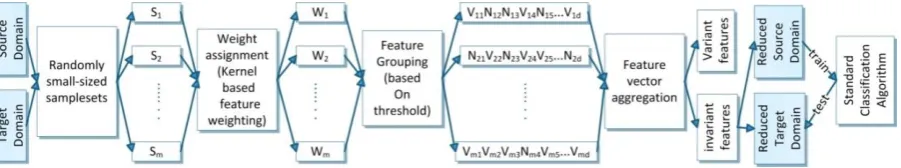
In this paper, we aim to find a solution to the problem of domain shift in datasets with large number of features and examples. The proposed approach is composed of five major steps: i) dividing the samples into random, small-sized, samplesets, ii) assigning weight to each feature of samplesets according to the kernel based feature weighting and instance clustering approach, iii) grouping features of each sampleset into different local categories (variant/invariant) regarding their weights obtained from the former phase, iv) aggregating the local variant and invariant feature vectors from different samplesets to compose ultimate vectors, and v) reducing datasets to the new representation and classifying target data using the standard machine learning algorithms. We omit the last step for brevity, as it is the same as learning any other classifier. Figure 1 shows the phases of RAkET in a graphical view.
Fig. 1. A graphical view of RAkET. Si is the ith sampleset and Wi is the diagonal weight matrix.
RAkET assigns a weight to each feature in local samplesets and categorizes features into the invariant (N) or variant (V) based on a threshold parameter
a) Kernel based feature weighting
Our objective is to discover the features whose distributions are invariant across domains. This implies that, we look for the features that minimize the distance between the source and target domains. Assume and are source and target matrices containing n and m
number of instances respectively and d number of features. The point is to discover diagonal weight matrix W, in such a way that the distance between the source and the target samples after reduction by the weight matrix stays as similar as possible. Distance measurement of two domains can be done by MMD. Utilizing MMD, learning W can be expressed as an optimization problem. Henceforth, the issue changes to discover W in such a way that the distance between domains is minimized:
(4)
where diag(W) is the diagonal of the weight matrix. The constraints control the range of W; the first constraint restricts the size of weights, and the second one allows W to only has positive values. Following Pan et al., 2011, the above equation can be rewritten in the form below using the kernel trick, i.e. ( ) where k is a positive definite kernel:
(5)
where
[
] (6)
and is a composite kernel matrix. , and are kernel matrices that have been defined by k on the source, target and cross domains respectively. is the coefficient matrix with , and . Each element in K is computed using the kernel function, thus they depend on W, e.g. using the polynomial kernel, with the degree p is calculated as .
b) Composing compact clusters in the reduced domains
The Eq. (5) finds W fully unsupervised while the source domain contains class labels that can be used for weighting the features to increase the classification performance. Since the source domain has the labeled instances, we could exploit this knowledge to improve the weight matrix. In finding W, the weights are adjusted in a way that the examples from same class have lower distance compared to their class means. This can be done through minimizing the distance between the examples of each class and their means. In this way, every instance falls in one compact cluster, hence, the classification performance increases. This yields the optimization problem:
(7)
where Q is an n×d matrix that contains the distance of each instance from its class mean in the source domain. Q can be computed as the following relation:
(8)
where denotes the source domain data sorted by class number in ascending order, and
distance between the reduced samples of each class and their means. It is worth noting that β is the regularizer that is adjusted through experiments.
Equation (7) is the reformulated optimization problem, which clusters instances in finding W. For simplicity, we use indicator matrix F, which contains zero and ones as elements for variant and invariant features, respectively. Algorithm 1 shows the achievement process of F. Actually, after solving the optimization problem, optimal weight matrix W* is used for generating the indicator matrix F.
Algorithm 1. The construction process of indicator matrix F using weight matrix W*
Input: Optimal weight matrix W*, number of samplesets m, number of features d, threshold parameter λ
Output: Indicator matrix F (m×d) for i = 1 to m do
w = diag(Wi*);
for j = 1 to d do if wj > λ then
Fi,j = 1; //invariant feature
else Fi,j = 0; //variant feature
-RAndom k-samplesETs (RAkET)
Feature selection for transfer learning (f-MMD) is a relatively simple method with the advantage of good accuracy on small-sized datasets. However, as briefly mentioned in the introduction of this article, f-MMD is challenged in domains with large number of features and examples. It is noteworthy that in some experiments, MMD cannot solve the problem and dismisses the results. In fact, the main challenge of f-MMD is its computation time, typically in datasets with large number of examples and features.
The computational complexity of f-MMD depends on the optimizer that solves the problem. In practice, interior-point optimizers like SeDuMi (Self-Dual Minimization) and SDPT3 (SemiDefinite Programming - Tutuncu, Toh, Todd) solve problems in 10 to 100 iterations. In uncommon cases in which the problem needs more than 200 cycles, numerical issues ordinarily keep them from solving the problem. Every cycle obliges polynomial complexity like O(n4.5) where n is the quantity of variables. In datasets with large number of features and examples, the number of variables in the optimization problem increases dramatically and raises the computation time of the algorithm.
In order to deal with the aforementioned problem, RAkET offers to break down the source and target domains into the random, small-sized, samplesets. In fact, RAkET divides the dataset into a number of samplesets, which are distinct from each other. In this situation, local feature categorization is done in each sampleset. Actually, RAkET seeks variant and invariant features in small-sized samplesets instead of the original dataset. Hence, we expect to solve the problem in a reasonable time with decreasing the complexity of the algorithm. Ultimately, all results from different samplesets are aggregated together to form the final solution.
RAkET offers advantages over f-MMD for several reasons. First of all, the resulting k-samplesets classification tasks are computationally simpler. Actually, RAkET by dividing the dataset to the random, small-sized samplesets, decreases domain adaptation time complexity. Also, it provides the ability to solve the problems with large number of features and instances. In addition, the resulting dataset has two major properties: i) lowest discrepancy in featuresets, and ii) maximum relation between invariant features and class labels. On the other hand, the performance of classifier increases by keeping the dependency between features and labels. In what follows, we introduce RAkET in further detail.
Given k being defined as the size of samplesets, RAkET initially partitions n samples randomly into
m=[n/k] disjoint samplesets, Sj, where j=1, …, m, ⋂ . Samplesets Sj, where j = 1, …, m-1 are
k-samplesets. If n/k is an integer, then sampleset Sm is also a k-sampleset, otherwise Sm contains the
Each vector contains the local variant and invariant features of samplesets and their aggregation compose the final vector of features.
Si is the i th
sampleset of the source and target domains. We assume that the number of samples in both domains are equal and define the k as the percentage of data from domains. The source and target domains indicated by S should be divided into m samplesets. This process proceeds in random and each sample is assigned to the individual Si. Ultimately for each sampleset, indicator matrix Fi is calculated using Eq. (7).
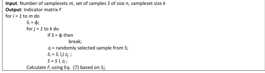
Algorithm 2 offers an algorithmic presentation of the learning process of RAkET.
Algorithm 2. The learning process of RAkET
Input: Number of samplesets m, set of samples S of size n, sampleset size k
Output: Indicator matrix F
for i = 1 to m do
Si = φ;
for j = 1 to k do if S = φ then
break;
zj = randomly selected sample from S;
Si = Si⋃ ;
S = S \ zj ;
Calculate Fi using Eq. (7) based on Si;
There are m vectors of local variant and invariant features, which are distinct from each other. In the next phase, each Fi should be aggregated to compose the final variant and invariant vectors. The final
vectors contain ultimate invariant and variant features of the dataset, which will be used for dataset reduction and classifier training. Algorithm 3 shows the aggregation process of RAkET, while Table 1 exemplifies it for a run with k = 20% and 7 features.
Algorithm 3.The aggregation process of RAkET
Input: Number of samplesets m, indicator matrix F, number of features d
Output: Variant and invariant features of dataset (V and N respectively)
N = φ;
V = φ;
for j = 1 to d do
sumj = 0;
for i = 1 to m do for j = 1 to d do
sumj = sumj + Fi,j;
for j = 1 to d do
avgj = sumj / m;
if avgj < 0.5 then
V = V⋃ ; else N = N ⋃ ;
Table 1. An example of the aggregation process of RAkET while k = 20% and d=7. For each sampleset Si, each
feature obtains variant (specified by 0) or invariant (specified by 1) tag, and ultimately the final tag is assigned with respect to results aggregated from different samplesets
Sampleset f1 f2 f3 f4 f5 f6 f7
S1 0 1 1 0 1 1 1
S2 0 0 1 0 1 1 0
S3 0 1 1 1 0 1 1
S4 0 1 0 1 1 1 0
S5 0 1 0 0 1 1 0
average votes 0/5 4/5 3/5 2/5 4/5 5/5 2/5
5. EXPERIMENTS
This section provides details on the experiments and results of the proposed approach. Section 5a introduces the artificial and real world datasets used by RAkET and Section 5b shows the evaluation measures and the basis of the comparison. Empirical results and analysis are presented in Section 5c and ultimately the comparison of RAkET with other transfer learning approaches is illustrated in the last section.
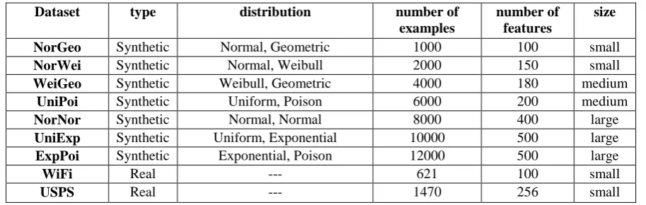
Experiments are conducted on 9 domain shift datasets where Table 2 presents the basic statistics such as type, distribution, size and number of examples and features of the datasets. We assume that the number of source and target examples is the same. Generally, the datasets are divided into the synthetic and real world. Synthetic datasets have been generated to test our approach in different conditions. We designed datasets with a variety of distributions and samples to show the performance of RAkET against f-MMD and other transfer learning methods. Real world datasets naturally have differences in distribution, and they are sufficient for the evaluation of domain shift problem. However, we categorize datasets regarding their size into three groups: small, medium and large. Most of the algorithms can handle small- and medium-sized datasets, but we will show that RAkET presents good performance on all types of datasets. Short descriptions of these datasets are given in the following paragraphs.
Table 2. Details of synthetic and real world benchmark transfer learning datasets
Dataset type distribution number of
examples
number of features
size
NorGeo Synthetic Normal, Geometric 1000 100 small
NorWei Synthetic Normal, Weibull 2000 150 small
WeiGeo Synthetic Weibull, Geometric 4000 180 medium
UniPoi Synthetic Uniform, Poison 6000 200 medium
NorNor Synthetic Normal, Normal 8000 400 large
UniExp Synthetic Uniform, Exponential 10000 500 large
ExpPoi Synthetic Exponential, Poison 12000 500 large
WiFi Real --- 621 100 small
USPS Real --- 1470 256 small
In order to generate the synthetic datasets, invariant and variant features should be sampled from different distributions to model the domain shift problem. The number of invariant and variant features is indicated by N and V, respectively. Dataset NorNor is a shifted dataset, which has been composed of the source and target domains where total number of features is 400. For both domains, N invariant features are sampled from N randomly picked distributions with zero mean and unit variance. For the source domain, V variant features are sampled from V randomly picked distributions with zero mean and unit variance. For the target domain, V variant features are sampled from V randomly picked distributions with shifted mean and unit variance.
Dataset WeiGeo is generated similar to NorNor with the difference being that for both domains N
invariant features and for source domain V variant features are sampled from randomly picked Weibull
distribution, and for the target domain V variant features are sampled from randomly picked Geometric
We then assess RAkET on real world datasets. Our first evaluation is on the task of indoor WiFi localization utilizing the general population WiFi information set distributed in the 2007 IEEE ICDM Contest for transfer learning. The objective of indoor WiFi localization is to anticipate the location of WiFi gadgets focused around Received Signal Strength (RSS) qualities gathered amid diverse time periods. Dataset contains a number of labeled WiFi information gathered in time period A (the source domain) and numerous unlabeled WiFi information gathered in time period B (the target domain).
Another real world dataset is USPS digit handwritten data. This dataset contains pictures of size 16 x 16, totaling up to 256 features, with pixel qualities going from 0 to 2. Numerous past works on the USPS dataset show that separating 4 from 7 [21] and 4 from 9 is especially difficult [22, 23]. In our experiments, digits 4 and 7 are considered as the source domain, and digits 4 and 9 are supposed to be the target domain. The classification task is binary and our goal is to discriminate information somewhere around 4 and 7 in the source to 4 and 9 in the target domain.
a) Evaluation metrics
There are two common criteria for evaluation of the classification methods, which are called execution time and accuracy. However, in this work for improving the legibility of the figures and simplifying the interpretation of the results, we use the percentage of improvement over f-MMD across several different datasets. Also, for real world dataset of WiFi localization, the average performance is calculated using the Average Error Distance (AED):
∑
where xi, f(xi) and yi are vectors of RSS values, predicted location and correspond to true location
respectively.
The linear SVM and logistic regression algorithms are used as the base-level classification methods where they are chosen in order to capture the contribution of each feature independently. The Weka [24] is used as the platform of classification algorithms and implementation of domain shift methods are done within Matlab [25].
b) Empirical results and analysis
In this section, the evaluation is based on the execution time and accuracy measures, estimated in 7 synthetic and 2 real world datasets. The first part of this section examines the performance of RAkET in synthetic datasets according to the size of the samplesets, k. The last part compares the performance of RAkET in real world datasets against f-MMD.
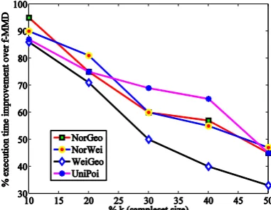
In this section, the improvement of RAkET against f-MMD is evaluated according to the different parameters. Figure 2 presents the percentage of improvement of RAkET over f-MMD in terms of execution time and accuracy with respect to the size of the samplesets (k) in small- and medium-sized synthetic datasets. Since f-MMD fails to run on large-sized datasets, Figure 2 does not include the results of large-sized dataset. The horizontal axis indicates the size of the samplesets (k) and points to the percent of data, which parts from the original dataset.
plausible explanation for the fact that RAkET's predictive performance is always increasing with respect to k (except in certain special circumstances). Nevertheless, values of k that are close to 10% of data perform well in terms of execution time. Ultimately, we could claim that setting k to small values is expected to lead to substantial better results in execution time against f-MMD, especially in datasets with large number of examples.
(a) Percentage of execution time improvement of RAkET over f-MMD. With increasing the size of samplesets, the performance of RAkET in terms of execution time degrades.
(b) Percentage of accuracy improvement of RAkET over f-MMD (linear SVM classifier). The classification accuracy increases with the increasing value of k.
(c) Percentage of accuracy improvement of RAkET over f-MMD (logistic regression classifier). The classifier shows better results for values more than k=30%.
Figures 2b and 2c present the percentage of accuracy improvement of RAkET over f-MMD using different classifiers with respect to various amounts of k in small- and medium-sized synthetic datasets. What we observe is that as the number of instances increase in the samplesets, so does the performance of the method. As before, this is due to the fact that a bigger value of k leads to more accuracy for each sampleset. An important finding that holds for all datasets is that the improvement of performance only exhibit for certain values of k. In most cases a good approximation for k is 40%.
In some cases, RAkET shows abnormal behavior with increasing the value of k. For example, consider the value of k is set to 50%. In this situation, the number of samplesets is 2, and there is the probability of uncertainty. On the other hand, if the assigned tags to a feature in distinct samplesets are different (e.g. one of them is variant and the next is invariant), decision making for determining the type of feature is done randomly. In general, because RAkET uses voting for feature grouping, odd number of samplesets show better performance.
Figure 3 shows the performance of RAkET in dealing with the large-sized datasets, on which f-MMD fails to run. The algorithm of f-MMD is computationally expensive, because it is a Quadratically Constrained Quadratic Program (QCQP), which can be cast as a Semi Definite Program (SDP). Figure 3a shows the execution time of RAkET in dealing with large-sized datasets. With incrementing the size of samplesets, RAkET spends more time to solve the problem. In fact, large-sized samplesets impose more variables to solve in the optimization problem.
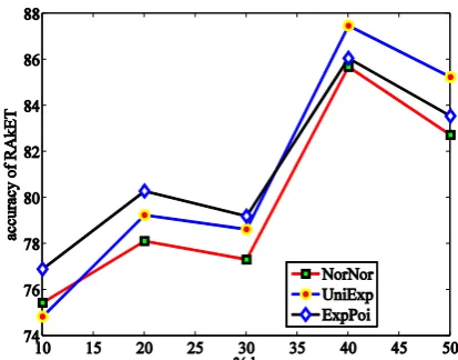
Figures 3b and 3c present the accuracy of RAkET using linear SVM and logistic regression classifiers with respect to different amounts of k in large-sized synthetic datasets. What is clear is that as the value of k increases, the accuracy of RAkET augments dramatically. In fact, samplesets with the large number of instances inherit more properties of the original dataset and categorize variant and invariant features more accurately. An important finding that holds for all datasets is that with a greater quantity of examples in samplesets, the performance of RAkET exhibits substantial improvement. But it must be noted that an even number of samplesets decreases the performance because it poses hindrance in the process of decision making.
We then evaluate our approach on the real world datasets. Figure 4a illustrates the performance of RAkET in case of real datasets against f-MMD. Small values of k decrease the running time of algorithm, but according to Figs. 4b and 4c the accuracy of classifier degrades likewise. One thing to note, however, is that the procedure of selecting the group for each feature via voting, as indicated, could lead to a case where none of the groups can be selected. In this situation, selecting an odd number of samplesets lessens the likelihood of getting no votes from the model. Also, as guideline, we suggest using a suitable value for
k (e.g. k = 40%).
c) Comparison with other methods
In this section, the evaluation is based on the accuracy measure, estimated via 10 repeated holdout experiments, each using the source domain of each dataset for training and the target domain for the evaluation. So, in this case RAkET is run a total of 10 times, as 10 different random datasets are used for each different holdout experiment. To calculate the performance of RAkET for a specific holdout experiment, we average the values obtained from these 10 executions.
attention. Ultimately, we compare RAkET against a generalized Fisher based method for Domain Shift problem, called FIDOS [26] that is a state-of-the-art approach.
(a) Execution time of RAkET in large-sized datasets. RAkET reduces runtime by breaking down the large-sized dataset into the small-sized samplesets.
(b) Accuracy of RAkET in large-sized datasets (linear SVM classifier). The classifier accuracy is reduced by decreasing the value of k.
(c) Accuracy of RAkET in large-sized datasets (logistic regression classifier). In most cases, RAkET shows better performance in large-sized samplesets.
a) Percentage of execution time improvement of RAkET over f-MMD. In real datasets the execution time of RAkET is raised with increasing the size of samplesets
(b) Absolute ridge regression error improvement of RAkET in WiFi dataset.
(c) Accuracy improvement of RAkET over f-MMD in USPS dataset (linear SVM classifier).
Fig. 4. Percentage of improvement of RAkET over f-MMD with respect to k in real world datasets
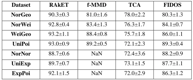
Tables 3 and 4 show the average and standard deviation of accuracy measure for all method-dataset pairs for synthetic datasets. As evident from the results, RAkET shows better performance against other transfer learning approaches. Likewise f-MMD and FIDOS show a more preferable accuracy over TCA, however with expanding the quantity of examples, f-MMD fails to run (NaN). Table 5 demonstrates the results of experiments on WIFI and USPS datasets. On both datasets, experiments show that RAkET significantly overcomes other transfer learning methods.
Table 3. Comparative results in terms of accuracy using linear SVM classifier. In all synthetic datasets, RAkET shows better performance against other transfer learning approaches. In datasets
with large number of instances, f-MMD fails to run (NaN)
Dataset RAkET f-MMD TCA FIDOS
NorGeo 90.3±0.3 81.0±1.6 78.0±2.2 80.3±1.3
NorWei 92.8±0.4 83.4±1.3 76.3±1.7 84.1±0.7
WeiGeo 93.2±1.1 88.4±0.8 75.7±1.8 86.0±1.1
UniPoi 93.0±0.9 89.2±0.5 72.1±2.3 89.3±0.4
NorNor 88.7±0.6 NaN 72.4±3.6 88.2±0.9
UniExp 89.7±0.7 NaN 73.1±1.5 87.7±1.1
ExpPoi 92.1±1.5 NaN 72.0±2.9 86.3±1.2
Table 4.Comparative results in terms of accuracy using logistic regression classifier. In all synthetic datasets, RAkET shows better performance against TCA,f-MMD and FIDOS. In datasets
with large number of instances, f-MMD fails to run (NaN).
Dataset RAkET f-MMD TCA FIDOS
NorGeo 88.1±0.3 77.4±0.9 76.5±1.4 76.6±1.0
NorWei 90.7±0.6 78.4±1.1 76.0±1.9 77.2±1.1 WeiGeo 90.0±0.9 82.1±0.6 74.7±2.1 77.1±0.9 UniPoi 93.1±0.5 85.2±0.8 70.9±0.8 78.0±0.7
NorNor 85.5±1.1 NaN 71.1±2.5 75.0±1.4 UniExp 89.2±0.9 NaN 72.8±1.7 77.9±0.7
ExpPoi 90.5±0.4 NaN 73.0±2.6 78.1±0.8
Table 5. Comparative results in terms of absolute error distance and accuracy in real world datasets. First row indicates average absolute ridge regression error on indoor WiFi localization dataset. Second
row shows the classification accuracy on the USPS dataset using linear SVM classifier.
Dataset RAkET f-MMD TCA FIDOS
WiFi (AED) 80.3±2.4 85.5±4.1 101.2±5.6 91.2±2.6
USPS 86.6±0.3 83.2±2.4 46.8±3.2 72.9±2.2
d) Conclusion and future work
samplesets, and employs kernel based feature weighting approach to learn invariant features. Moreover, the proposed method benefits from the instance clustering to enhance the classification performance in the reduced domains. RAkET improves the execution time of f-MMD about 50% while the accuracy has growth at an acceptable level. On benchmark tasks in both synthetic and real world problems, our method consistently outperforms other transfer learning methods. For future work, we plan to advance in this direction further, e.g. proposing RAkET for multi domain setting.
REFERENCES
1. Lu, J., Behbood, V. Hao, P., Zuo, H., Xue, S. & Zhang, G. (2015). Transfer learning using computational
intelligence: A survey. Knowledge-Based Systems, Vol. 80, pp. 14-23.
2. Fakhrahmad, S. M., Rezapour, A. R., Sadreddini, M. H. & Zolghadri Jahromi, M. (2014). A novel approach to
machine translation: A proposed language-independent system based on deductive schemes. Iranian Journal of
Science and Technology-Transactions of Electrical Engineering, Vol. 38, No. E1, pp. 59-72.
3. Blitzer, J., McDonald, R. & Pereira, F. (2006). Domain adaptation with structural correspondence learning.
Proceedings of the conference on empirical methods in natural language processing, pp. 120-128. Association
for Computational Linguistics.
4. Uguroglu, S. & Carbonell, J. (2011). Feature selection for transfer learning. In Machine Learning and
Knowledge Discovery in Databases, pp. 430-442. Springer.
5. Gretton, A., Borgwardt, K. M., Rasch, M., Schölkopf, B. & Smola, A. J. (2006). A kernel method for the two
-sample problem. In Advances in neural information processing systems, pp. 513-520.
6. Gopalan, R., Li, R. & Chellappa, R. (2014). Unsupervised adaptation across domain shifts by generating
intermediate data representations. Pattern Analysis and Machine Intelligence, IEEE Transactions on, Vol. 36,
No. 11, 2288-2302.
7. Hoffman, J., Kulis, B., Darrell, T. & Saenko, K. (2012). Discovering latent domains for multisource domain
adaptation. In Computer Vision-ECCV, pp. 702-715. Springer.
8. Gong, B., Shi, Y., Sha, F. & Grauman, K. (2012). Geodesic flow kernel for unsupervised domain adaptation. In
Computer Vision and Pattern Recognition (CVPR), 2012 IEEE Conference on, pp. 2066-2073. IEEE.
9. Ben-David, S., Blitzer, J., Crammer, K., Pereira, F. & et al. Analysis of representations for domain adaptation.
Advances in neural information processing systems, Vol. 19, No. 137.
10. Duan, L., Tsang, I. W., Xu, D. & Maybank, S. J. (2009). Domain transfer svm for video concept detection. In
Computer Vision and Pattern Recognition. CVPR 2009. IEEE Conference on, pp. 1375-1381. IEEE.
11. Long, M., Wang, J., Sun, J. & Yu, P. S. (2015). Domain invariant transfer kernel learning. Knowledge and Data
Engineering. IEEE Transactions on, Vol. 27, No. 6, pp. 1519-1532.
12. Jiang, J. & Zhai, C. X. (2007). Instance weighting for domain adaptation in nlp. In ACL, Vol. 7, pp. 264-271.
Citeseer.
13. Mansour, Y., Mohri, M. & Rostamizadeh, A. (2009). Domain adaptation with multiple sources. In Advances in
neural information processing systems, pp. 1041-1048.
14. Huang, J., Gretton, A., Borgwardt, K. M., Schölkopf, B. & Smola, A. J. (2006). Correcting sample selection bias
by unlabeled data. In Advances in neural information processing systems, pp. 601-608.
15. Gretton, A., Smola, A., Huang, J., Schmittfull, M., Borgwardt, K. & Schölkopf, B. (2009). Covariate shift by
kernel mean matching. Dataset shift in machine learning, Vol. 3, No. 4, p. 5.
16. Gong, B., Grauman, K. & Sha, F. (2013). Connecting the dots with landmarks: Discriminatively learning
domain-invariant features for unsupervised domain adaptation. Proceedings of the 30th International Conference
17. Pan, S. J., Kwok, J. T. & Yang, Q. (2008). Transfer learning via dimensionality reduction. In AAAI, Vol. 8, pp.
677-682.
18. Gheisari, M. & Soleymani Baghshah, M. (2015). Unsupervised domain adaptation via representation learning
and adaptive classifier learning. Neurocomputing.
19. Pan, S. J., Tsang, I. W., Kwok, J. T. & Yang, Q. (2011). Domain adaptation via transfer component analysis.
Neural Networks, IEEE Transactions on, Vol. 22, No. 2, pp. 199-210.
20. Baktashmotlagh, M., Harandi, M. T., Lovell, B. C. & Salzmann, M. (2013). Unsupervised domain adaptation by
domain invariant projection. In Computer Vision (ICCV), IEEE International Conference on, pp. 769-776.
21. Xu, Z., King, I., Lyu, MR-T. & Jin, R. (2010). Discriminative semi-supervised feature selection via manifold
regularization. Neural Networks, IEEE Transactions on, Vol. 21, No. 7, pp. 1033-1047.
22. Sugiyama, M., Idé, T., Nakajima, S. & Sese, J. (2010). Semi-supervised local fisher discriminant analysis for
dimensionality reduction. Machine learning, Vol. 78, Nos. 1-2, pp. 35-61.
23. Zeng, H. & Cheung, Y. M. (2009). Feature selection for local learning based clustering. In Advances in
Knowledge Discovery and Data Mining, pp. 414-425, Springer.
24. Hall, M., Frank, E., Holmes, G., Pfahringer, B., Reutemann, P. & Witten, I. H. (2009). The weka data mining
software: an update. ACM SIGKDD explorations newsletter, Vol. 11, No. 1, pp. 10-18.
25. The Math Works Inc. (2012b). Matlab and statistics toolbox release. Natick, Massachusetts, United States.
26. Dinh, C. V., Duin, R. P. W., Piqueras-Salazar, I. & Loog, M. (2013). Fidos: A generalized fisher based feature
extraction method for domain shift. Pattern Recognition, Vol. 46, No. 9, pp. 2510-2518, 2013.