1.
Introduction
The flow of natural gas through transmission pipelines is transient due to the changes in demand conditions during a 24-h cycle, pressure fluctuations at the stations, changes in operating conditions, and other factors. Natural gas pipelines are often buried underground; therefore, their internal flow can be supposed to be isothermal. In addition, the flow has relatively low speed and therefore the gas has enough time to reach a thermal equilibrium with its surroundings; this is another reason for assuming the problem as an isothermal flow.
Natural gas transmission lines are often long, and the important parameters in their design are typically the longitudinal pressure gradient (pressure drop) and the flow rate. Because the main changes in this kind of flow are longitudinal variations, the problem is mostly studied using a
one-dimensional approach, and changes in radial direction are neglected. Therefore, the friction effects between the fluid (gas) and pipe walls are modelled as an algebraic term and added to the right-hand side of the governing equations, making them nonhomogeneous.
Considering the above-mentioned assumptions, the governing equations for the transient flow of natural gas through pipelines are hyperbolic in nature. The exact solutions of these equations are very important in the design and control of lines in gas transport networks. To achieve more accurate results, either a first-order method on a fine grid or a scheme with a high order of accuracy on a coarse mesh can be used. Some of the research using the former approach is discussed below.
Zhou and Adewumi [1] presented a new Total Variation Diminishing (TVD) method for solving differential equations of unsteady one-dimensional
Numerical Simulation of Transient Natural Gas Flow in Pipelines Using
High Order DG-ADER Scheme
Ali Falavand Jozaei
*,a, Ali Tayebi
b, Younes Shekari
b, Ashkan Ghafouri
aa Department of Mechanical Engineering, Ahvaz Branch, Islamic Azad, University, Ahvaz, Iran
b Department of Mechanical Engineering, Yasouj University, Yasouj, Iran
A B S T R A C T
To increase numerical accuracy in solving engineering problems, either conventional methods on a fine grid or methods with a high order of accuracy on a coarse grid can be used. In the present research, the second approach is used and the arbitrary high-order DG-ADER method is applied to analyze the transient isothermal flow of natural gas through pipelines. The problem is investigated one dimensionally. and the effect of friction force between the pipe wall and fluid flow is considered as a source term on the right-hand side of the momentum equation. Therefore, the governing equations have a hyperbolic nature. Two real problems with associated field data are simulated using this method. The results show that highly accurate results can be obtained using the DG-ADER method, even on a coarse grid. Furthermore, the conventional small-amplitude oscillations of DG-ADER method do not appear in the transient natural gas flow due to the smoothness of the flow field properties.
© 2017 Published by Semnan University Press. All rights reserved. DOI: 10.22075/jhmtr.2016.497
PAPER INFO History:
Submitted: 2016-04-22 Revised: 2016-11-07 Accepted: 2016-11-25
Keywords:
Numerical Simulation; DG-ADER method; Natural gas; Pipe flow; Transient flow.
Journal of Heat and Mass Transfer Research
Journal homepage: http://jhmtr.journals.semnan.ac.ir
Corresponding Author: Ali Falavand, Department of mechanical engineering, Ahvaz branch, Islamic Azad University, Ahvaz, Iran
flow of natural gas through a horizontal pipe without neglecting the inertia term of the momentum equation. Other researchers have neglected the inertia term in the momentum equation to simulate the unsteady flow of natural gas in pipelines. That neglect changed the governing differential equations from nonlinear to linear. The earlier numerical methods, the explicit and implicit finite difference methods, and the method of characteristics lead to results that are far from precise because the inertia term in the momentum equations is disregarded.
Osiadacz [2] evaluated different models of unsteady flow simulation. He pointed out that the numerical simulation of partial differential equations, which represents a dynamic model of a network, requires a numerical method with high accuracy and low computational time to obtain trustworthy results. Ibraheem and Adewumi [3] proposed a numerical procedure to simulate the unsteady two-dimensional flow of gas; they used a particular Runge–Kutta method to determine accurate flow properties.
Mohitpour et al. [4] reported the importance of studying unsteady flow in designing and optimizing gas transmission lines; they showed that the simulation of steady flow was suitable when changes in demand were stable. In general, the simulation of steady flow is accurate enough when there are no dramatic changes in the mass flow rate. However, the mass flow rate changes over time, making the unsteady flow model more appropriate in simulating fluid flow.
Tao and Ti [5] studied unsteady flow through gas transmission lines using an analogy between electrical circuit parameters and gas networks. Based on their study and due to daily consumption peaks, it is possible to have a situation in which the available equipment is unable to maintain adequate system pressure. Therefore, it is necessary to decrease the pressure at certain points of the network to equalize the pressures at other points. Using a transfer function model and MATLAB Simulink, Behbahani-Nejad and Bagheri [6] examined the transient flow of natural gas through pipelines and gas networks. Behbahani-Nejad and Shekari [7] carried out a reduced order modelling of the transient flow of natural gas through pipelines using the flux vector splitting method and the eigenvector approach.
As mentioned, to achieve a precise solution for fluid flow simulation problems, either a first-order method on a fine grid or a high-order method on a
coarse grid can be used. Obviously, using a fine grid causes a round-off error problem and increased computational cost. Therefore, the second technique seems to be more appropriate. As a consequence, researchers are often looking for methods with a high order of accuracy to carry out their simulations. Unfortunately, simulations using high-order methods have some constraints, such as high fluctuations in properties at flow field discontinuities. According to the Godunov theorem [8], there is no linear method that has an order higher than one and that is monotone. In this theorem, the point is the linearity of the method. Therefore, if a nonlinear method is used, the Godunov theorem is not valid and a monotone method may be employed.
Following the Godunov theorem, many nonlinear methods have been proposed by other researchers. The TVD method and the Monotonic Upwind Scheme for Conservation Laws (MUSCL)– Hancock technique are two of those methods [9]. Despite the many advantages of these methods, the ultimate accuracy that can be achieved is second-order accuracy, and achieving a higher accuracy is impossible. To overcome this problem, Titarev and Toro [10, 11] invented the Arbitrary DERivative (ADER) method, which can provide any arbitrary order of accuracy. This method is actually an extension of the MUSCL–Hancock technique in order to achieve a higher order of accuracy for numerical solutions.
knowledge, however, this method has not been applied in solving issues relating to the flow of isothermal transient natural gas. In this research, the DG-ADER method is used to investigate the transient one-dimensional flow of isothermal natural gas through pipelines.
2. Governing equations and constitutive
relations
The flow of isothermal natural gas through a pipeline can be described using the following set of partial differential equations (PDEs) [1]:
𝜕𝐐 𝜕𝑡 +
𝜕𝐄(𝑸)
𝜕𝑥 − 𝐇(𝐐) = 0 (1)
where
𝐐 = (𝜌𝑢) , 𝑬 = (𝜌 𝜌𝑢2𝜌+ 𝑝) , 𝑯 = (
0 −𝜌𝑓𝑔
𝑢|𝑢| 2𝐷
) (2)
in which 𝜌, 𝑢, 𝑓𝑔, 𝑝, and 𝐷 are the density, velocity, friction factor, pressure, and diameter of the pipe, respectively. The isothermal and isentropic gas equation of state is used to relate the density of the gas to its pressure, as follows:
𝑝 = 𝜌𝐶2 (3)
where C is the speed of sound.
3.
Numerical method
In the present research, the DG-ADER method is used for the numerical simulation of the flow field. Using this method, any arbitrary order of accuracy with controlled spurious oscillations can be achieved. This method involves three main steps. In the first step, reconstruction is performed using the weighted essentially non-oscillatory (WENO) scheme. In the second step, the time evolution is performed to calculate a high-order space–time polynomial. In the third step, the data obtained in the second step is used to compute the conservative variables of the flow (i.e., 𝐐 in Eq. (1)), using the finite volume scheme; the reader is referred to references [2-4] for more details. Some general and key points of the method are briefly presented below.
The one-step finite volume discretization of Eq. (1) over the space–time control volume
[xj−1/2, xj+1/2] × [tn, tn+1] reads as:
q̅jn+1= q̅ j
n−∆t
∆x(Fj+1
2
− Fj−1 2
) + ∆tSjn, (4)
where ∆x = [xj−1/2, xj+1/2] and ∆t = [tn, tn+1]. The average value of a finite volume cell, q̅jn, is defined
as follows:
q̅jn=
1
∆x∫ q(x, t
n)dx
xj+1/2
xj−1/2
(5)
and the integrals of numerical flux at the cell boundaries and source terms are defined as appear in the following equations:
𝐹𝑗+1 2
=
1
∆𝑡∫ 𝑔 (𝑞ℎ(𝑥𝑗+12
− , 𝑡) , 𝑞 ℎ(𝑥𝑗−1
2 + , 𝑡)) 𝑑𝑡
𝑡𝑛+1
𝑡𝑛 and
(6)
Sj= 1
∆t∆x∫ ∫ S(qh(x, t))dxdt
xj+1/2
xj−1/2
tn+1
tn . (7)
In Eq. (6), g(Q−, Q+) is a classical Riemann solver (e.g., Rusanov scheme; see (5) for more schemes). Furthermore, qh is a local space–time predictor from the space of piecewise space–time polynomials of degree N. This function is computed using a local weak form of the governing equations (1) on an element. More details about the related procedure can be found in [3-4-6].
Some important points of the DG-ADER method are described briefly, as follows. First, the governing system of PDEs (1) is transformed to a local space–time reference element, TE= [0; 1] ×
[0; 1] with coordinates ξ and τ, where x = xi−1/2+
ξΔx and t = tn+ τΔt. Second, the obtained system of PDEs is multiplied by the space–time test function θk(ξ, τ). Third, an integration operator of the resultant system of equations over TE is performed. Employing integration by parts for the time derivative term, one can obtain the following relationship:
[θk, qh]T1i− 〈 ∂
∂τθk, qh 〉Ti+
〈θk, ∂
∂ξf ∗(q
h) 〉Ti− 〈θk, S∗ (qh)〉Ti=
[θk, whn]Ti
0,
(8)
where
[a, b]Tτi = ∫ a(ξ, τ)b(ξ, τ)dξ 1
0
,
〈a, b〉Ti= ∫ ∫ a(ξ, τ)b(ξ, τ)dξdτ 1
0 1
0
(9)
and
f∗
h(ξ, τ) = Δt
ΔxF(qh),S
∗
h(ξ, τ) = ΔtS(qh). (10)
polynomial. A similar notation as that used in [3] is employed for the WENO scheme. It is assumed that the WENO reconstruction polynomials are given by the following series:
𝑤ℎ𝑛= 𝑤ℎ(𝑥, 𝑡𝑛) = ∑𝑁+1𝑙=0 𝜓𝑙(𝑥)𝑤̂𝑙𝑛,
(11)
where N is the polynomial degree of reconstruction and ψl represents the reconstruction basis functions. Here, the Legendre polynomials are used as the space basis functions. In Eq. (11), ŵln are expansion coefficients.
For the element local predictor solution qh, the cell boundaries fluxes, f∗
h, and the source term,
S∗
h, the following relationships are used. In these relationships, the Einstein summation rule over two repeated indices is used.
qh(ξ, τ) = ∑ θl(ξ, τ)
(N+1)2
l=1
q̂l= θlq̂l,
f∗
h(ξ, τ) =
Δt
ΔxF(qh) = ∑ θl(ξ, τ)
(N+1)2
l=1
fl
= θlf̂l,
S∗h(ξ, τ) = ΔtS(qh) = ∑ θl(ξ, τ)
(N+1)2
l=1
Ŝl
= θlŜl.
(12)
Substituting the above relationships into Eq. (8) and performing some mathematical manipulations, one can obtain the following equation:
[θk, θl]1Tiq̂l− 〈 ∂
∂τθk, θl 〉Tiq̂l+
〈θk, ∂
∂ξθl 〉Tif̂l− 〈θk, θl 〉Ŝl= [θk, ϕ]Ti
0 ŵ
l.
(13)
In the compact matrix form, Eq. (13) can be rewritten as follows:
K1q̂lm+1− MS∗(q̂m+1l ) = f0ŵl− Kξf∗(q̂lm), (14)
in which
𝐾1= [𝜃𝑘, 𝜃𝑙]𝑇𝑖
1 − 〈𝜕
𝜕𝜏𝜃𝑘, 𝜃𝑙 〉𝑇𝑖,
𝐾𝜉= 〈𝜃𝑘, 𝜕
𝜕𝜉𝜃𝑙 〉𝑇𝑖,
𝑀 = 〈𝜃𝑘, 𝜃𝑙 〉𝑇𝑖, 𝑓0= [𝜃𝑘, 𝜙]𝑇0𝑖.
(15)
In the recent relationships, M is the mass matrix, K_1, K_ξ represents the temporal and spatial stiffness matrices, and f_0 is the flux matrix. By solving Eq. (14) and obtaining q ̂_l, the conservative variable q_h can be computed using Eq. (12).
Equation (14) is also solved using an iterative procedure. It can be shown that the solution is converged after N+1 iterations.
The main steps in the implementation of the DG-ADER method are as follows:
1) Nonlinear (non-oscillatory) reconstruction of spatial polynomials from the given cell averages at time t^n.
2) Local solution for the initial value problem (14) inside each element, where the initial data is given by the spatial reconstruction polynomial at time t^n.
3) Numerical integration of the integrals in equations (6) and (7) and updating of the cell averages according to Eq. (4).
4.
Results
To evaluate the DG-ADER method in analyzing the natural gas transient flow through pipelines, two real examplesof available field data are simulated. These problems are also investigated in reference [19] and analyzed by Zhou and Adewumi [1] and Behbahani-Nejad and Shekari [7].
Fig. 1: Schematic of the first studied problem
First point
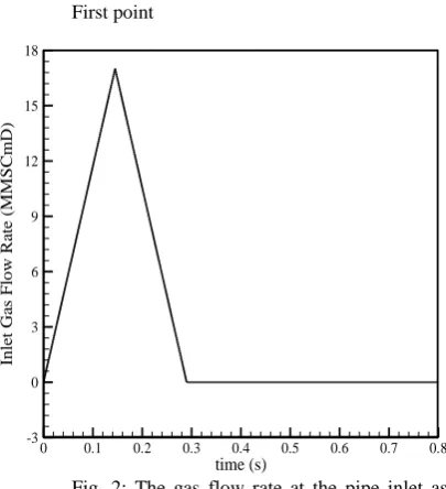
Fig. 2: The gas flow rate at the pipe inlet as a function of time for the first case
time (s)
In
le
t
G
a
s
F
lo
w
R
a
te
(M
M
S
C
m
D
)
0 0.1 0.2 0.3 0.4 0.5 0.6 0.7 0.8 -3
Test case 1: Injection of natural gas into a
closed-end pipe
A pipe with a length of 91.44 m and a diameter of 0.61 m is plugged at its end and an internal pressure of 4.136 MPa is maintained. A a triangular pulse is imposed on the inlet to change the inlet mass flow rate (Fig. 1). The total simulation time of the test is 0.8 s. The pulse is such that the inflow rate is linearly increased from zero at the initial time to 17 MMSCmD in 0.145 seconds and then decreased to zero in 0.145 seconds. The sound speed and friction factor are 348.1 m/s and 0.03, respectively.
The resulting pressure at the pipe inlet is shown in Fig. 3 and is compared with the result of the flux vector splitting (FVS) method of Steger and Warmming used by Behbahani-Nejad and Shekari [7]. The results of both methods are also compared with the field data. It is observed that very good results are obtained using a fourth-order DG-ADER method on a grid of 100 cells. The obtained pressure distribution is almost closed to the field data and is slightly better compared to using the FVS method on the same computational grid.
The pressure changes versus time for the pipe endpoint are compared with the results of the FVS method [7] and field data in Fig. 4. Good agreement between the present results and field data and slightly better results compared to the results of the FVS method at the endpoint are observed. It is shown that the pressure does not change with time first; an increase in pressure is observed when the wave of the injected gas meets the pipe endpoint, and then a pressure drop is obtained after gas wave reflection (Fig. 4).
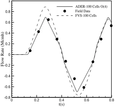
The standard volumetric flow rate changes during the time in the middle section of the pipe are also measured (Fig. 5). The ability of the DG-ADER method to predict the volumetric flow rate changes can be clearly seen in Fig. 5. An increasing trend in the volumetric flow rate is observed as the gas wave approaches the middle section. As the wave passes from this section, the flow rate decreases. The reflected wave causes a negative flow rate at this section.
Fig. 3: Pressure changes at the pipe inlet
Fig. 4: Pressure changes at the pipe endpoint
Fig. 5: Changes in the mass flow rate at the middle section of the pipeline
t(s)
p
(M
P
a
)
0 0.2 0.4 0.6 0.8
4.1 4.2 4.3 4.4 4.5
ADER-100 Cells-O(4) Field Data FVS-100 Cells
t(s)
p
(M
P
a
)
0.2 0.4 0.6 0.8
4.1 4.2 4.3 4.4 4.5
ADER-100 Cells-O(4) Field Data FVS-100 Cells
t(s)
F
lo
w
R
a
te
(M
c
m
h
)
0 0.2 0.4 0.6 0.8
-0.8 -0.6 -0.4 -0.2 0 0.2 0.4 0.6 0.8 1
Fig. 6: The effect of increasing the numerical method accuracy on the pressure distribution of the endpoint
Fig. 7: The effect of increasing the numerical method accuracy on flow rate changes in the middle point of the
pipe
Fig. 8: Mass flux at the outlet section of the second test case
Fig. 9: Pressure versus time at the pipe outlet on a 1000-cell grid using the DG-ADER method with different
accuracy and the FVS method compared with the field data
One of the major challenges of the DG-ADER method is numerical fluctuations with limited amplitude in the flow field discontinuity locations. In the studied problem, inherent fluctuations of the DG-ADER method do not appear due to the lack of discontinuities in the flow filed.
To evaluate the effect of increasing numerical accuracy on the results, pressure changes at the pipe endpoint and flow rate changes in the middle point of the pipe are investigated using a 100-cell grid and are shown in Fig.s 6 and 7, respectively. It is observed that the higher the numerical accuracy, the greater the accuracy of the results and the better the agreement between the numerical results and the field data.
Test case 2: The gas pipeline with known
outlet mass flow rate
A pipe system of 72259.5 m in length and 0.207 m in diameter with natural gas flow with 0.675 specific gravity and 10 ºC in temperature is simulated as the second case [20]. The gas viscosity and pipe roughness height are 11.84×10⁻⁶ kg.m-1s-1 and 0.6kg.m-1s-17 mm, respectively. Because there are no initial conditions, the steady state conditions are considered as the initial conditions for the problem. The friction factor is supposed to be constant for the duration and equal to the corresponding steady state value. Relating to the boundary conditions, the inlet pressure is set to be constant, whereas at the pipe outlet a change of flow rate (Fig. 8) is imposed due to the demand changes during a day. This problem is also studied by Zhou and Adewumi [21] using a TVD method, by Tentis et al. [22] using the method t(s)
p
(M
P
a)
0.2 0.4 0.6 0.8
4.1 4.2 4.3 4.4 4.5
100 Cells-O(2) 100 Cells-O(3) 100 Cells-O(4) Field Data
t(s)
F
lo
w
R
a
te
(M
c
m
h
)
0 0.2 0.4 0.6 0.8
-0.8 -0.6 -0.4 -0.2 0 0.2 0.4 0.6 0.8
ADER-100 Cells O(2) ADER-100 Cells O(3) ADER-100 Cells O(4) Field Data
time (hours)
G
a
s
M
a
ss
F
lu
x
(k
g
/(
m
2 s)
)
0 2 4 6 8 10 12 14 16 18 20 22 24 90
95 100 105 110 115 120 125 130 135 140
t(hr)
p
(M
P
a)
0 4 8 12 16 20 24
0.5 1 1.5 2 2.5
3 DG-ADER-1000 Cells-O(2)
of lines and an adaptive mesh, and by Behbahani-Nejad and Shekari [7] using the FVS method.
Pressure changes versus time at the end section of the pipe are shown in Fig. 9 and compared with the field data and the results of the FVS method on a 1000-cell grid. It is observed that the results of the third and fourth order of the DG-ADER method are in good agreement with field data. An increase and a drop in pressure at the outlet are observed due to the demand flow rate increase and decrease, respectively. It is also shown that the third and fourth order of the DG-ADER method can predict the maximum outlet pressure very well.
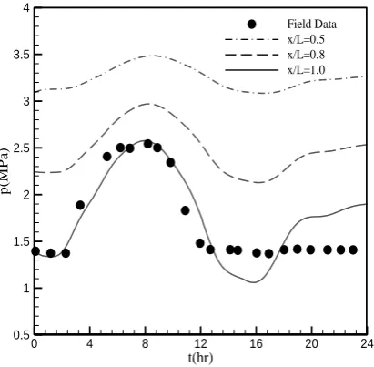
Pressure distribution at different sections of the pipe is shown in Fig. 10. It is observed that the pressure at different sections changes by the same trend; however, the effect of change in the mass flow rate at the outlet section is sensed at any point at a time proportional to the distance from the outlet.
The outstanding point in these two cases is that there are no low-amplitude fluctuations in the obtained results. One feature of the DG-ADER method is limiting (but not completely eliminating) the amplitude of the fluctuations. However, there is no fluctuation in these two cases because the physics are such that no discontinuity happens in their flows. Therefore, there is no place for oscillations to appear in the flow fields. Therefore, the DG-ADER method seems to be a very good method for analyzing real transient problems.
Fig. 10: Pressure versus time in different sections of the pipe using a third-order DG-ADER method on a 100-
cell computational grid
Fig. 11: Pressure distribution along the pipe at different times
Pressure distribution along the pipe at different times is shown in Fig. 11. Comparing the results with those of Zhou and Adewumi [22], the ability of the DG-ADER method in this research to simulate transient flow problems of natural gas through pipelines is observed.
5.
Conclusion
The DG-ADER method is a novel method to reach any arbitrary order of accuracy in space and time. In the present research, this scheme was used for the numerical simulation of transient natural gas flow through pipelines. After describing the governing equations and required constitutive relationships, the DG-ADER method was described briefly. Two real problems were simulated using the DG-ADER scheme up to a fourth order of accuracy. The results showed that the DG-ADER method can be used to simulate transient natural gas flows with good accuracy, even on coarse meshes.
One of the main shortcomings of the DG-ADER method is the appearance of very small amplitude oscillations near the flow discontinuities. The results showed that there were no spurious oscillations in the transient natural gas flow in pipes because the physics are such that no discontinuity happens in this type of flow. Therefore, there is no place for oscillations to appear in flow fields. Consequently, this method is recommended for use in the numerical simulation of natural gas flow in pipelines.
t(hr)
p
(M
P
a
)
0 4 8 12 16 20 24
0.5 1 1.5 2 2.5 3 3.5 4
Field Data x/L=0.5 x/L=0.8 x/L=1.0
Distance (km)
P
re
ss
u
re
(M
P
a
)
0 10 20 30 40 50 60 70
0.5 1 1.5 2 2.5 3 3.5 4 4.5
Nomenclature
C speed of sound D diameter of the pipe F0 flux matrix
fg friction factor
𝑓∗ℎ cell boundary fluxes
K1 temporal stiffness matrix
Kξ spatial stiffness matrix
M mass matrix p pressure
𝑆∗
ℎ source term t time
u velocity
𝑤̂𝑙𝑛 expansion coefficients ρ density
ψl reconstruction basis functions
References
[1].Zhou, J., Adewumi, M., 1995, “Simulation of
transient flow in natural gas pipelines”. 27th Annual Meeting Pipeline Simulation Interest Group (PSIG).
[2].Osiadacz, A.J., 1996 “Different Transient Flow
Models-Limitations, Advantages, And Disadvantages”, PSIG Annual Meeting, Pipeline Simulation Interest Group.
[3].Ibraheem, S., Adewumi, M., 1996, “Higher
resolution numerical solution for 2-D transient natural gas pipeline flows”, SPE Gas Technology Symposium, Society of Petroleum Engineers.
[4].Mohitpour, M., Thompson, W., Asante, B., 1996, “The importance of dynamic simulation on the design and optimization of pipeline transmission systems.” American Society of Mechanical Engineers, New York, NY (United States).
[5].Tao, W., Ti, H., 1998, “Transient analysis of gas
pipeline network.” Chemical Engineering Journal, 69(1): pp. 47-52.
[6].Behbahani-Nejad, M., Bagheri, A., 2010, “The accuracy and efficiency of a MATLAB-Simulink library for transient flow simulation of gas pipelines and networks” Journal of Petroleum Science and Engineering, 70(3): pp. 256-265.
[7].Behbahani-Nejad, M, Shekari, Y., 2010, The accuracy and efficiency of a reduced-order model
for transient flow analysis in gas pipelines. Journal of Petroleum Science and Engineering, 73(1–2): pp. 13-19.
[8].Godunov, S.K., 1959, “Finite difference methods
for the computation of discontinuous solutions of the equations of fluid dynamics”. Mathematics of the USSR, 47: pp. 271–306.
[9].Toro, E.F., 2005, Riemann Solvers and Numerical Methods for Fluid Dynamics, 3rd ed.,: Springer, Manchester.
[10].Titarev, V., Toro, E.F., 2002, “ADER:
Arbitrary high order Godunov approach” Journal of Scientific Computing, 17(1-4): pp. 609-618.
[11].Titarev, V., Toro, E.F., 2005, “ADER schemes
for three-dimensional non-linear hyperbolic systems”, Journal of Computational Physics, 204(2): pp. 715-736.
[12].Dumbser, M., Balsara, D. S., Toro, E.F., Munz, C.D., 2008, “A unified framework for the construction of one-step finite volume and discontinuous Galerkin schemes on unstructured meshes”. Journal of Computational Physics, 227: pp. 8209-8253.
[13].Dumbser, M., Enaux, C. and Toro, E.F., 2008, “Finite volume schemes of very high order of accuracy for stiff hyperbolic balance laws”, Journal of Computational Physics, 227: pp. 3971-4001.
[14].Dumbser, M., Hidalgo, A., Castro, M., Pares, C., Toro, E.F., 2010, “FORCE schemes on unstructured meshes part II: Non-conservative hyperbolic systems”, Computer Methods in Applied Mechanics and Engineering, 199(9): pp. 625-647.
[15].Dumbser, M., Kaser, M., Titarev, V., Toro, E.F., 2007, “Quadrature-free non-oscillatory finite volume schemes on unstructured meshes for nonlinear hyperbolic systems”, Journal of Computational Physics, 226: pp. 204-243.
[16].Taube, Dumbser, M., Balsara, D. S., Munz, C.D., “Arbitrary high-order discontinuous Galerkin schemes for the magnetohydrodynamic equations”, Journal of Scientific Computing, 30(3): pp. 441-464.
[17].Shekari, Y. Tayebi, A., 2015, “Numerical simulation of two-phase flows, using drift flux model and DG-ADER scheme” Modares Mechanical Engineering, 15(9): p. 51-58.
[18].Dumbser, M., 2011, “Advanced Numerical
Methods for Hyperbolic Equations and Applications” 2011: Trento.
[19].Dempsey, R.J., Rachford, H.H., Nolen, J.S., 1972, “Gas Supply Analysis-States of the Arts”, AGA Conf. San Francisco.
[20].Taylor, T. D., Wood, N. E. and Power, J. E., 1962, "A Computer Simulation of Gas Flow in Long Pipelines," Soc. Pet. Eng, Trans, AIME, vol. 225, pp. 297-302
(PSIG), pp. 18-20
[22].Tentis, E., Margaris, D., and Papanikas, D., 2003, "Transient gas flow simulation using an