An Optimal Tax Relief Policy with Aligning Markov Chain and Dynamic Programming Approach
Ali Mohammadi Shiraz University, Shiraz [email protected]
Ahmad Rajabi Shiraz University, Shiraz [email protected]
Abstract
In this paper, Markov chain and dynamic programming were used to represent a suitable pattern for tax relief and tax evasion decrease based on tax earnings in Iran from 2005 to 2009. Results, by applying this model, showed that tax evasion were 6714 billion Rials**. With 4% relief to tax payers and by calculating present value of the received tax, it was reduced to 3108 billion Rials. With regard to transition periods of tax-receipt and its discount index, the present value of future tax cash flows, during the future period, were 16034 billion Rials. Also, by means of dynamic programming, the break–even-point of tax relief index was determined. Consequently, if the discount rate were less than 22%, the optimal policy to increase tax revenue would be not to give discount and if it were more than 22%, the favorable policy would be to offer discount to tax payers.
Keywords: Markov Chain, Transition Period, Tax Relief, Dynamic
Programming
JEL Classification: G14- C21 - C22 - C53 - D84
1. Introduction
Many complexities and changes created in phenomena in the last decade led to an uncertainty and unpredictable behavior. These changes in economic and social systems are more than other systems. Markov Chain is a special case of random possible processes in which the condition of the system is just dependent on the last previous state. This model is able to calculate transitionprobabilities from one stage to other stages.
Reviews of received taxes show that parts of taxes are not gathered constantly in the due time and some are received with delay. First, it shows that the process of tax receipt is with a degree of probability. Second, part of receiving tax lasts to the next year during the transition period. So, the result would be an increase in tax evasion. Obviously, with these conditions, choosing an appropriate tax- policy can increase the reception rate in the due time and reduce the tax evasion.
For this purpose, with respect to the Markovian transition tax process and Dynamic Programming approach, a good model for decision-making in tax relief is introduced in four stages. In the first step, with regard to processes of receivable tax in 2005-2009, the algorithm transition was determined based on Markov chains. In the second step, steady state received tax and fundamental matrix were calculated. In the third step, receivable tax was calculated in the no relief policy, and relief policy. The results of the two states were compared. In the fourth step, by dynamic programming and relief policy, tax relief index was determined and optimal decision was taken.
2. Literature Review
Markov chain method has had numerous applications in various sectors such as agriculture, climate change, medicine and engineering. In the recent decade, the uses of Markov chain in the social and economic systems, especially in financial sectors, have found a suitable situation.
Brown (1965) used dynamic programming and transition probabilities for optimal decision making in tax relief in the US banks. This method decreased tax evasion compared to previous methods.
individual rates cycle.
Plassman and Tideman (2000) used Markov chain and Monte Carlo simulations to estimate the parameters in determining the effective tax rates for housing construction in Pennsylvania, USA in 1972 to 1994. The results showed that using this method to determine tax relief rate in future periods provided more useful information than other possible ways for decision-making.
Another research related to tax evasion subject and Markov chain was by Hanousek (2002). The main focus of the study was on estimating transition probabilities between the state of tax evading and not evading. In this research, non-panel surveys were conducted in 2000, 2002, and 2004. He used a dataset of 1062 individuals from the Czech Republic to forecast the evolution of tax evasion in that country. Respondents were asked whether they evaded never, sometimes, or frequently. This information was collected to classify individuals as evaders or non-evaders. It was concluded that the estimate of the shift allowed guessing how people might move between the categories of tax evading and not evading in the next five years and a small decrease in tax evasion would be seen then.
Derang & Cheng (2003) used Markov chain method to determine the pattern of facilities for credit institutions to customers in China. The application of Markov chain resulted in providing information for managers of this organization to determine policy guidelines to payment loans and to determine an appropriate credit policy to customers in the next periods.
Piunovskiy(2006) proposed a suitable pattern to analyze and decide appraisal with aligned dynamic programming and Markovian chain. This method applies in many countries for tax relief, special in East European countries.
claim that the quality of government services and the level of corruption matter mightily. Clearly, other factors also matter, including the size and ownership of the firm, the fairness of the legal system, the level of competition, the tax rate, the quality of the bureaucracy, and the expectation of audits.
Saibeni (2010) used Markov chain method to predict receivable accounts in American companies. He compared different methods and concluded that Markov chain method was more useful to predict the process of collecting the receivable accounts than the other ones. Unlike Markov chain, in other methods, the transition periods of receivable accounts were not taken into consideration.
These studies represent the efficiency of Markov chain and dynamic programming in diverse contexts. This study attempted to work on this aspect in order to facilitate the way to increase tax receipt.
3. Methodology 3.1 Markov Chain Process
Markov chain is a special case of probability model. In this model, the current system state is only dependent on the last level. If a set of Markov processes is considered as the following, it is at any moment, one of the distinctive modes of S1……S(n). State of the system in discrete times and regular distances changes with a set of probabilities. If the state is shown as (qt) for (t=1, 2…n) in (t) time, to express the performance of this process in the form of Markov chain, It was needed to know the current state according to previous cases that is shown in the relation below:
P(qt=Sj)
(1)
In this model:
P (qt) represents the system state.
P (qt = Sj | qt-1) represents the conditional probabilities transition.
3.1.1 System State
System state specifies its position in a time period, such as, paid or unpaid taxes. For example, if the system time is zero, the mode is shown as below:
P (0) = [P1 (0), P2 (0), P3 (0)] (2) In this relation:
P (0) = vector quantities Pi (0) for different modes.
P1 (0) = the probability that the system in zero time be in state1. P2 (0) = the probability that the system in zero time be in state 2. P3 (0) = the probability that the system in zero time be in state 3.
So, if it is assumed that the system at zero time is in state 1. Then, P (0) = [1, 0, 0]. Likewise, if the system in zero time is in state 2, then, P (0)=[0,1,0] or if the system is in state 3, then, it will be P(0)=[0,0,1]. With the use of these conditions, in Markov processes, the transition states can be defined.
Since, in Markov process, the system state at any time is dependent on the previous mode, probability transitions with regard to (n) periods is defined as below:
p(n)=p(0)pn=[p1(n),p2(n),…pi(n)]=[p1(0),p2(0),…pm(0)] (3) P(n)= Vector mode in (n) time
P(0)= Vector mode in (0) time n= Number of time periods 0 =The initial condition m= Number of possible states
3.1.2 Transition Probabilities
Transition probabilities represent the move from a state to the other state during a specified period. These changes are related to the current state. For example, the probability that in the previous state, tax had not been paid, and in this period, would be paid is related to the previous state. It is shown as a conditional probability.
Pij = Pr {X1 = j | X0 = i} (4) According to space state of S = {0, 1, 0}
If possible probabilities are considered as P (ij), in line with conditions and probabilities in Markov chain, the transition matrix is defined as:
(5)
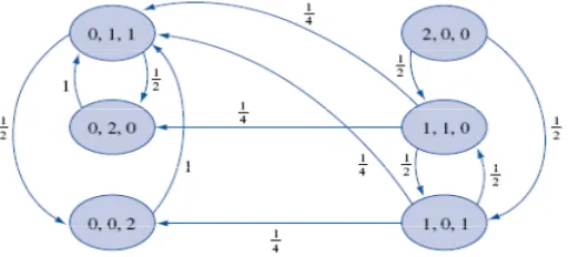
According to this matrix, transition probabilities are moving from mode 1 to (i) to the one of the states of 1 to (j). In this model, for example, the probability that the system is in state 1 and transits to state 1 is shown with P(11). The probability that the system is in (i) state and transits to state (j) is shown with P(ij). If the probability of changes is considered between 6 modes, it can be said that probability that the system be in zero state and would stay in it is zero. The probability that the system be in zero state and transits in state 2 is equal to 0.5 Eventually, the probability that the system be in state 2 and transfer to the zero mode will be equal to 1. Since, in this matrix, the transition probability is only possible from state 2 to zero state, it is called "absorbing state”(state 1, 4, 5, and 6). ( Maskin and Taylor, 2001). (Figure 1).
1 2 3 0 0 0 i
P11 P12 P13……..P1j
P21 P22 P23 ……P2j
P31 P32 P33……P3j
… …. …. ….
… …. …. ….
…. …. …. ...
Pi1 Pi2 Pi3 Pij
Pij=
3… …….j 2
Figure 1. Transition processes between state 0, 1 and 2
3.2 Dynamic Programming Method
Dynamic programming is one of the best operation research methods for solving complex problems by breaking them down into a sequence of decision steps. This is done by defining a sequence of value functions f1,
f2, ..., fn, with an argument Srepresenting the state of the system at times i
from 1 to n. The definition of fn(S) is the value obtained in state Sat the
last time n. The values fi at earlier times i=nQ1,nQ2, ..., 2, 1 can be
found by working backwards, using a recursive equation. For i= 2, ...,n, fiQ1at any state Sis calculated from fiby maximizing a simple function of
the gain from decision iQ1 and the function fi at the new state of the
system if this decision is made. Since fi has already been calculated for
the needed states, the above operation yields fiQ1for those states. Finally,
f1 at the initial state of the system is the value of the optimal solution. optimal decision in this stage was calculated using the following formula:
{
( , )}
max )
( k n n
n i f s v
f = (6)
Recursive equation determined such that:
{
( )}
max )
(i v f 1 i
f k n s
i k
n = + + (7)
) (i fn
= The optimal decision in stage n.
k i
3.3 Aligning dynamic programming with Markovian chain
With regard to Markovian chain, suppose Ps is the transition matrix associated with the S stationary policies, S=1, 2, 3…S. s
i
V is expected revenue of policy Sfrom state i, i=1,2,..m. Based on the above relation, expected revenue of policy S per transition step is calculated with this formula:
i s s i m
i
S p v
E =
=
1
(8)
The optimum policy for *
s is determined with:
{ }
SS Max E
E * = (9)
Optimal policy for each stage includes the optimization of the current stage and the previous stage. Therefore, the recursive function, in this model, includes the optimization of the current stage and the prior stage. If instead ofES apply f (i)
n and k=stage, then value determination each step is calculated:
{
( )}
max )
( 1
1
j f p v
i
f s
n k ij m
j k i k
n +
= +
= (10)
In this equation: )
(i fn
= The optimal expected revenue of stage n.
k i
V = optimal decision in stage (n-1).
) (
1 1
j f p n
k il m
j
+ =
= Optimal decision value in stage (n) according to
conditions of possible tax receipt.
To calculate the present received value, by use of discount factor (0< S<1), the recursive equation can be written as:
) (i
fn =Max { 1( )
1
j f p
V k n
ij m
j k
i +
=
+ } (11)
3.4 Application of Markov Chain and dynamic programming for Tax Relief Pattern
One of the major challenges of tax receipt, in our country, is non-complete receipt of anticipated tax. On the other hand, part of tax in each period is not received in the due time. This issue causes the increasing risk of tax receipt and it will affect the value of future received payments. Considering features of Markov chain method, in this model, “state” represents the present tax receipt situation. Transition probabilities represent time process of tax receipt in different parts. (Yaniv,1994).
To calculate, according to tax receipt transition matrix based on Markov chain, this matrix is divided into four separate sections as follows:
I O
Pij = ... (12)
R Q
In this matrix, I= unit matrix, O= zero matrix, R= matrix of transition probabilities which in next periods reaches to the absorbing state and Q= matrix of transition probabilities between all states of non- absorb.
Considering the defined matrix, the basic step to identify the behavior of this system is to compute the fundamental matrix. The fundamental matrix is calculated as below:
F= (I-Q) 1 (13)
In this matrix, for example, the first month shows that if tax receipt transfers to the first month, 10% is likely that this tax is going to be received in the first month, 20% in the second month, 10% in the fourth month, 14% in the seventh month and 5% in the ninth month.
1 0 0 0 0 0 0 0 0 0 0 0 0 0 .56 .30 0 .1 0 0 .04 0 0 0 0 0 0 0 .45 .25 0 0 0 0 0 .2 0 0 0 .1 0 0 .45 .35 0 0 0 0 0 .15 0 0 0 .1 0 .05 .62 .21 .15 0 0 .03 0 .2 0 0 0 0 0 .46 .28 .18 0 0 .05 0 0 0 0 0 0 .02 .66 .22 .12 0 0 .0 0 0 0 0 0 0 .0 .40 .25 .3 0 0 .05 0 0 0 0 0 0 .05 .55 .20 .10 0 0 .05 0 0 0 0 0 0 .1 .3 .28 .12 0 0 .15 0 0 .25 0 0 0 .0 .75 .20 .0 0 0 .05 0 0 0 0 0 0 .0 0 .5 .0 .3 0 0 .15 0 0 0 0 0 0 .05 0 0 .21 .35 .4 .0 0 .04 0 0 0 0 0 0 0 0 0 0 0 0 0 0 0 0 0 0 0 0 0 1 R
1 2 3 4 5 6 7 8 9 10 11 12 E
Pij=
. . . . .
As the ultimate goal of this process is to reach a steady state, a fundamental matrix leads to a steady state. Considering the state of tax receipt transition matrix, the data were analyzed through QM software and were simulated in five year period. The results show the extent of tax receipt in future periods.
The following matrix shows the tax receipt in 13 state (1, 2, and 3…E) and five-year period (2005 - 2009). For example, in the first month in 2005, with the probability of 0.18, 3309 billion Rials were received and with 0.04 probabilities, 809 billion Rials would be non-receivable. Other tax receipt information during the transitional period is shown too.
.1 .2 0.1 0 0.14 0 .05 0 .0 .0 0 .4 0 0 0 0 0 0 .05 .2 0 0 0 0 0 .05 0 0 .0 . 1 .0 0 0 .03 0 0 0 0 .0 .2 .0 0 0 .05 0 0 0 0 .05 . 2 .10 0 0 .0 0 .05 0 .0 .25 .4 0 0 .05 0 0 .1 0 .05 . 0 . 0 0 0 .05 .12 0 0 .1 .0 .10 0 0 .1 0 0 0 0 0 .2 .0 0 0 .2 0 0 0 .01
F=
.18 .14 .12 .1 .11 .09 .08 .05 .02 .04 .03 .01 .04 .17 .15 .13 .11 .09 .08 .07 .06 .03 .05 .01 .02 .035
.21 .12 .12 .08 .09 .06 .06 .05 .03 .01 .02 .03.04 .17 . 13 .18 .17 .12 .1 .09 .08 .06 .09 .01 .02 .04
.15 .16 .14 .14 .13 .09 .08 .07 .05 .08 .07 .04 .04 2005
2006 2007 2008 2009
E 12 11 10 9 8 7 6 5 4 3 2 1
Year
1 2 3 4 5 6 7 8 9 10 11 12 E Total Tax Received
20 05 33 09 27 57 25 73 22 06 22 06 18 14 91 9 55 1 73 5 55 1 18 4 55 1 -8 09 17 54 9 20 06 38 16 33 67 29 18 22 45 20 20 17 96 15 71 13 47 67 3 10 10 22 4 44 9 -1 01 0 22 44 9 20 07 57 50 54 76 32 86 21 90 21 90 16 43 16 43 13 69 82 1 27 4 54 8 82 1 -1 36 9 27 38 1 20 08 62 96 59 65 53 02 33 14 33 14 19 88 18 23 99 4 10 11 33 1 64 6 66 3 -1 49 1 33 13 7 20 09 76 31 71 22 71 22 61 05 50 87 35 61 30 52 20 35 20 35 25 44 15 26 10 17 -2 03 5 50 87 2
Total -6714
According to tax relief policy, to determine the index of tax relief, this pattern is reviewed again. With tax relief policy, tax receipt increases. As tax payers will benefit from tax relief, part of tax will not be received from them. For example, with tax relief in the first month, the probability of earning revenue increases from18% to 22% and the earned revenue increases from3309 billion Rials to 4165 billion Rials. Also in the whole examined period, the probabilities of not earning revenue decreases from4% to 1% and the earning revenue decreases from 809 billion Rials to 379 billion Rials.
.22 .16 .15 .12 .12 .09 .11 .05 .02 .02 .01 .01 .01 .21 .17 .15 .13 .11 .09 .05 .03 .02 .02 .01 .01 .00 .22 .21 .18 .12 .09 .07 .04 .03 .01 .01 .01 .01 .01
year 1 2 3 4 5 6 7 8 9 10 11 12 E Total tax received 20 05 41 65 30 29 28 40 22 72 17 04 13 25 11 36 94 7 37 9 37 9 18 9 18 9 -3 79 18 93 3 20 06 48 56 39 31 34 68 27 75 25 43 18 50 11 56 69 4 46 2 46 2 23 1 23 1 -4 86 23 14 6 20 07 62 05 59 23 50 76 31 02 22 56 19 74 11 28 84 6 28 2 28 2 28 2 28 2 -5 64 28 20 2 20 08 68 26 64 85 61 44 40 96 27 30 17 07 17 07 13 65 10 24 34 1 68 3 34 1 -6 83 34 13 1 20 09 94 32 89 08 78 60 68 12 52 40 41 92 26 20 20 96 15 72 10 48 52 4 10 48 -9 96 52 34 6
Total -3108
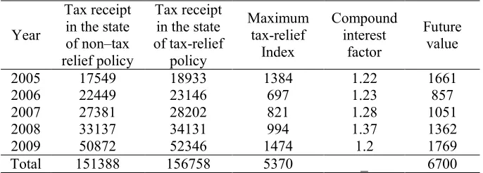
Results of taking this tax policy, based on tax relief and non-relief index during 2005-2009 are shown in table 1. For example, based on the data in 2005, government can provide a discount of 1384 billion Rials to taxpayers. In this case, the relief-index will reach to break-even-point. For the other years, tax-relief index is shown in table 1.
Table 1: Comparison of tax receipt in the state of tax relief and non-tax relief policy - Billion Rials
Future value Compound interest factor Maximum tax-relief Index Tax receipt
in the state of tax-relief
policy Tax receipt
in the state of non–tax relief policy Year 1661 1.22 1384 18933 17549 2005 857 1.23 697 23146 22449 2006 1051 1.28 821 28202 27381 2007 1362 1.37 994 34131 33137 2008 1769 1.2 1474 52346 50872 2009 6700 _ 5370 156758 151388 Total
months in each year; present value of tax will be different in the transition. For this purpose, the Dynamic Programming method wasused to calculate the present value of the received tax and to appraise an optimal policy. The index used to calculate the present value of the tax is the real inflation rate including nominal inflation and interest rate. This index is applied to select optimal policy in dynamic programming. In this method, optimal policy, for each stage, includes the optimization of the current stage and the previous stage. Therefore, the recursive function, in this model, includes the optimization of the current stage and the prior stage. The optimal decision is calculated according to the following equation:
) (i
fn =Max { 1( )
1
j f p
V k n
ij m
j k
i +
=
+ }
In this equation: )
(i
fn = The optimal decision in stage (n) (each year as a stage of decision-making)
k i
V = optimal decision in stage (n-1).
= Rate of discount factor (real inflation rate).
) (
1 1
j f pk n
il m
j= +
= Optimal decision value in stage (n) according to
conditions of possible tax receipt
By using the above function, the value of received tax in 2005 - 2009, based on non-relief tax policy is calculated as the following. These results determine the selection of an optimal policy in each year.
f(2005)={.22f(1)+.16f(2)+.15f(3)+.12f(4)+.12f(5)+.09f(6)+.11f(7)+.05f
(8)+.02f(9)+ .02f(10)+.01f(11)+.01f(12)-.01f(13)}=17159
f(2006)=17159+{.21f(1)+.17f(2)+.15f(3)+.13f(4)+.11f(5)+.09f(6)+.05f
(7)+.03f(8)+ .02f(9) + .02f(10)+.01f(11)+.01f(12)-.00f(13)}=19893
f(2007)=19893+{.22f(1)+.21f(2)+.18f(3)+.12f(4)+.09f(5)+.07f(6)+.04f
(7)+.03f(8)+ .01f(9)+ .01f(10)+.01f(11)+.01f(12)-.01f(13)}=23985
f(2008)=23985+{.20f(1)+.19f(2)+.18f(3)+.12f(4)+.08f(5)+.05f(6)+.05f
(7)+.04f(8)+ .03f(9)+ .02f(10)+.01f(11)+.01f(12)+.01f(13)}=28678
f(2009)=28678+{.18f(1)+.17f(2)+.15f(3)+.13f(4)+.1f(5)+.09f(6)+.05f
Year
1 2 3 4 5 6 7 8 9 10 11 12 E
T ot al ta x re ce iv ed 20 05 32 56 28 71 25 53 20 69 20 37 16 49 82 8 48 5 63 7 47 0 15 4 45 5 -6 68 17 15 9 20 06 37 51 32 54 27 72 20 96 18 54 16 20 13 93 11 74 57 7 85 1 18 6 36 5 -8 22 19 89 3 20 07 56 33 52 55 30 88 20 17 19 76 14 52 14 22 11 61 68 2 22 3 43 6 64 1 -1 06 9 23 98 5 20 08 61 36 56 65 49 08 29 89 29 13 17 04 15 22 80 9 80 2 25 6 48 7 48 7 -1 09 5 28 67 8 20 09 75 15 69 07 68 02 57 41 47 12 32 48 27 42 18 00 17 73 21 82 12 89 84 6 -1 69 3 45 55 7
In addition, value of received tax, based on the tax relief policy, is as the following:
f(2005)={.18f(1)+.14f(2)+.12f(3)+.1f(4)+.11f(5)+.09f(6)+.08f(7)+.0
5f(8)+.02f(9)+ .04f(10)+.03f(11)+.01f(12)+.01f(13)}=17465
f(2006)=17465+{.17f(1)+.15f(2)+.13f(3)+.11f(4)+.09f(5)+.08f(6)+.0
7f(7)+.06f(8)+ .03f(9) + .05f(10)+.01f(11)+.02f(12)+.035f(13)}=21253
f(2007)=21253+{.21f(1)+.2f(2)+.12f(3)+.08f(4)+.09f(5)+.06f(6)+.05
f(7)+.03f(8)+ .01f(9)+ .02f(10)+.03f(11)+.01f(12)+.04f(13)}=25770
f(2008))=25770+{.19f(1)+.18f(2)+.17f(3)+.12f(4)+.1f(5)+.09f(6)+.0
8f(7)+.06f(8)+ .09f(9)+ .01f(10)+.02f(11)+.04f(12)+.03f(13)}=30434
f(2009)=30434+{.151f(1)+.16f(2)+.14f(3)+.14f(4)+.13f(5)+.09f(6)+.
year 1 2 3 4 5 6 7 8 9 10 11 12 E T ot al ta x re ce iv ed 20 05 38 99 28 34 27 01 21 32 15 73 12 04 10 16 83 3 32 8 32 3 15 9 15 6 -3 13 17 46 5 20 06 47 73 37 98 32 94 25 90 23 34 16 69 10 25 60 5 39 6 38 9 19 1 18 8 -3 95 21 25 3 20 07 60 78 56 83 47 72 28 56 20 35 17 44 97 6 71 7 23 4 22 9 22 5 22 0 -4 40 25 77 0 20 08 66 53 61 59 56 87 36 95 24 01 14 62 14 25 11 11 81 2 26 4 51 4 25 1 -5 01 30 43 4 20 09 92 88 86 39 75 06 64 07 48 53 38 23 23 53 18 54 13 69 89 9 44 3 87 2 -8 28 48 30 6
Results of these two policies are shown in the table below:
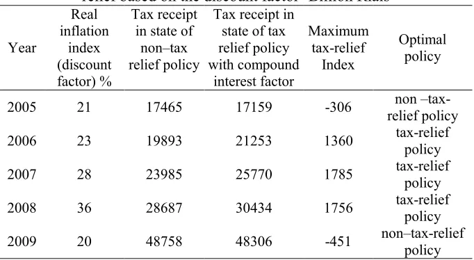
Table 2: Comparison of received tax in state of tax relief and non-tax relief based on the discount factor- Billion Rials
Optimal policy Maximum
tax-relief Index Tax receipt in
state of tax relief policy with compound
interest factor Tax receipt
According to the information in table 2 and selection of a best policy, an optimal decision based on the discount factor, the present value of the received tax and the tax relief will be different. In 2005 and 2009, the discount factor (21%, 20%) was less than tax relief (22%), the tax discount policy was not appropriate. However, in 2006, 2007 and 2008, the discount factor rate was more than the tax relief. Founded on the results of calculations, the rate of 22% is considered as the break-even-point. If the rate of the discount-factor is less than 22%, it is better to apply the policy of non-discount payment. But if the discount-factor rate is more than 22%, taking policies of tax relief would be desirable.
4. Discussion and Recommendation
One of the important challenges of government in tax income is to increase receipt of anticipated tax and to decrease tax evasion. For this purpose, various incentive policies can be used to receive tax in the due time to increase tax income. Taxes are one of the important sources of income in the developed countries but in developing countries tax evasion is a prevalent problem (Hanousek, 2007).
Now, in Iran, appropriate policies are not used for tax relief. Moreover, the present policies are subjective with no consideration of scientific models. For this, the study of tax-payers’ behaviors, tax discount rate in previous periods and their impacts on tax receipt can appropriately provide a model based on the present revenue value. In this paper, a desired pattern for future periods was presented with Markov chain attributes and dynamic programming in identifying characteristics of taxpayers’ behaviors and transition periods of tax receipt.
transitional period of tax receipt, the more the present value of future cash flows and the higher value for the government. By applying this policy, it is expected to reduce tax evasion. Hanousek, J, Palda and Easter (2007), in their research concluded that near to 40% of tax income was not received in European East countries.
Another important result of this study is the use of Dynamic Programming method and the implementation of the discount factor in order to take an appropriate policy of tax relief against non-relief tax. Based on the results of this method, the discount factor rate of 22% is considered as the break-even-point. If the discount factor is less than 22%, the optimal policy is no relief. But, by increasing the discount factor, and by reducing value of money, the appropriate policy is tax relief. As in this state, the present value of cash flows increases in the transitional period. Piunovskiy (2006) in her research in Russian perceived that the tax relief index for firms was near to 7% and for personal income was 4%. But in Poland tax relief index is different.
Appendix:
Appendix 2: Simulation process in transition period for received tax
Appendix 3: Transition matrix based on the first year 0.046677
State Initial State Probability Resulted State
Probability
State 1 0.492089 0.741258
State 2 0.241297 0.142168
State 3 0.125000 0.023877
State 4 0.018196 0.028505
State 5 0.005538 0.001922
State 6 0.046677 0.005799
State 7 0.003165 0.009652
State 8 0.008703 0.027714
State 9 0.004747 0.000198
State 10 0 0
The number of time periods from initial: 1
Appendix 4: Transition matrix based on the total years and stationary state
References
Brown, W., (1965). On the iterative method of dynamic programming on a finite space discrete time markov process. The Annals of Mathematical Statistics, 36(4), 25-32.
Derang, H., & Cheng, H.C., (2003). Using markov chains to estimate losses from a portfolio of mortgages. Review of Quantitative Finance and Accounting, 12(3), 303-318.
Engel, M.R., & Hines, J. R., (1999). Understanding tax evasion dynamics. England. National Bureau of Economic Research.
Hanousek, J., (2002). The evaluation of tax evasion in the Czech Republic: a markov chain analysis. Journal of Public Economic, 36, 57-72.
Hanousek, J., Palada, H., & Easter, R., (2007). Appraisal impact of confidence firms to government on tax evasion in the east European countries with markov chain analysis. Journal of Tax Review, 4,25-51. Maskin, E., & Taylor, J., (2001). Markov perfect equilibrium, observable
actions. Journal of Economic Theory, 100,191-219.
Saibeni,A.,(2010). Forecasting accounts receivable collections with markov chains. The CPA Journal, 33, 1-12.
Plassmann, F., & Tideman, T.N., (2000). A markov chain monte carlo analysis of the effect of two-rate property taxes on construction. Journal of Urban Economics, 47, 216-247.
Piunovskiy, A.B., (2006). Dynamic programming in constrained markov decision processes. Control and Cybernetics Journal, 35(3), 11-14. Yaniv, G., (1994). Tax evasion and the income tax rate: A theoretical