Two-fluid compressible simulations on GPU cluster

J.-S. Dhersin, Editor

TWO-FLUID COMPRESSIBLE SIMULATIONS ON GPU CLUSTER

Philippe Helluy

_{and Jonathan Jung}

Abstract. In this work we propose an efficient finite volume approximation of two-fluid flows. Our scheme is based on three ingredients. We first construct a conservative scheme that removes the pressure oscillations phenomenon at the interface. The construction relies on a random sampling at the interface [5, 6]. Secondly, we replace the exact Riemann solver by a faster relaxation Riemann solver with good stability properties [4]. Finally, we apply Strang directional splitting and optimized memory transpositions in order to achieve high performance on Graphics Processing Unit (GPU) or GPU cluster computations.

Résumé. Nous proposons une méthode de volumes finis efficace pour l’approximation d’écoulements bifluides. Le schémas est basé sur trois ingrédients. Nous construisons d’abord un schéma conservatif sans oscillations de pression. La construction repose sur un échantillonnage aléatoire à l’interface. Ensuite, nous remplaçons le solveur de Riemann exact par un solveur approché de relaxation plus rapide, et qui possède de bonnes propriétés de stabilité. Finalement, nous appliquons un splitting directionnel de Strang et des techniques de transposition optimisées en mémoire pour atteindre de bonnes performances sur GPU ou cluster de GPU.

1.

Introduction

We are studying the numerical resolution of a two-fluid compressible fluid flow. The model is the Euler equations with an additional transport equation of a color functionϕ. The functionϕis equal to 1 in the gas and0 in the liquid. It allows locating the two-fluid interface. We consider the system

∂tW +∂xF(W) +∂yG(W) = 0, (1)

where

W = (ρ, ρu, ρv, ρE, ρϕ)T,

F(W) = (ρu, ρu2+p, ρuv,(ρE+p)u, ρuϕ)T, G(W) = (ρu, ρuv, ρv2+p,(ρE+p)v, ρvϕ)T.

The pressure lawpis a stiffened gas pressure law

p(ρ, e, ϕ) = (γ(ϕ)−1)ρe−γ(ϕ)p∞(ϕ), (2)

1 _{IRMA, University of Strasbourg; [email protected]} 2 _{IRMA, University of Strasbourg; [email protected].}

c

EDP Sciences, SMAI 2014

wheree=E−u2₊ v2 2 ,and

(γ, p∞)(ϕ) = (

(γgas, p∞,gas), ifϕ= 1,

(γliq, p∞,liq), ifϕ= 0.

Recall that the system (1) coupled with the pressure law (2) is hyperbolic on the domain

Ω : =

W = (ρ, ρu, ρv, ρE, ρϕ)∈R5, ρ >0,

ϕ∈[0; 1], p

ρ, E−u

2_+v2

2 , ϕ

+p∞(ϕ)>0

.

The main point is that the hyperbolic setΩis generally not convex ifp∞,16=p∞,2 (see [12]).

Classic conservative finite volume schemes generally produce an artificial diffusion of the mass fractionϕ. In the numerical approximation we may observe a mixture zone 1 > ϕ > 0. This artificial mixing zone implies a loss of velocity and pressure equilibrium at the interface. It is possible to recover a better equilibrium by relaxing the conservation property of the scheme as in [17].

Independently of the pressure oscillations, problem of stability appears for classic schemes. This comes from the non-convexity of the hyperbolic set Ω [12]. In this paper, we use a random sampling projection at the two-fluid interface. It allows preserving the non convex hyperbolic domain. The method was first proposed in [6] for a particular traffic flow model. It does not introduce a mixture zone and extends the one-dimensional method described in [2]. More precisely, we construct a numerical scheme that preserves the hyperbolic domain without diffusionH,

H:= Ω0∪Ω1, (3)

where for allϕ0∈[0; 1], the convex setΩϕ0 is

Ωϕ0: =

W = (ρ, ρu, ρv, ρE, ρϕ)∈R5, ρ >0,

ϕ=ϕ0, p

ρ, E−u

2_+v2

2 , ϕ

+p∞(ϕ)>0

.

2.

An ALE-projection scheme with a random numerical method

2.1.

_Introduction

In order to compute the two-dimensional numerical solution, we use dimensional splitting. It means that each time step is split into two stages. In the first stage we solve∂tW +∂xF(W) = 0and in the second stage

we solve ∂tW +∂yG(W) = 0. In addition, in our application, thanks to the rotational invariance of the Euler

equations, the two resolutions are equivalent if we simply exchange the space variables x and y and the velocity components u and v. It is thus enough to construct a scheme for solving the one dimensional system

∂tW+∂xF(W) = 0. (4)

We generalize the Lagrange-projection scheme. We replace the Lagrange step by an Arbitrary Lagrangian Eulerian step (ALE step). It allows us to switch between a Lagrangian approach at the liquid-gas interface and a Eulerian approach in the pure phases.

We want solve (4) on [a;b]×R+_{. We consider a sequence of times tn, n ∈} N _{such that the time step}

∆tn:=tn+1−tn >0.We consider also a space steph=b−_Na,whereN is a positive integer. We define the cell

centers byxi=a+ i+12

h, i= 0· · ·N+ 1.The cellCiis the interval i

x_i−1 2;xi+

1 2 h

,wherex_i+1 2 =xi+

ALE step:

h

Remapping step:

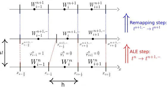
Figure 1. _{Structure of the ALE-projection scheme.}

now focus on an approximationWn

i ≈W(xi;tn).The boundary cellx_i+1

2 moves at speed

ξn i+1

2 between time

tn

andt−_n+1

xn+1,−

i+1 2

=x_i+1

2 + ∆tnξ n i+1

2

.

A time iteration of the ALE-projection scheme includes two steps (see Figure 1):

• the ALE step: withWn

i onCi, we obtainWin+1,− on the cellC n+1,−

i =

i xn+1,−

i−1 2

;xn+1,−

i+1 2

h ,

• a projection step to obtain the Euler variables at timetn+1 on the original cellCi.

We use the notation·n+1,− _{to characterize the value of ·at timet}−

n+1, just before the projection step.

2.2.

_{ALE step}

2.2.1. Finite volume scheme

Integrating the conservation law (4) on the space-time trapezoid

n

(x, t), x_i−1

2 + (t−tn)ξ n i−1

2 < x < xi+ 1

2 + (t−tn)ξ n i+1

2, tn< t < t

−

n+1

o ,

we obtain the finite volume scheme

h_in+1,−W_in+1,−=hW_in−∆tn

F(W_in, W_in₊₁, ξ_in₊1

2)−F(W n

i−1, Win, ξin−1 2)

, (5)

wherehn_i+1,−=xn+1,−

i+1 2

−xn+1,−

i−1 2

=h+ ∆tn(ξ_in₊1 2−

ξn i−1

2)and

F(WL, WR, ξ)is the conservative ALE numerical

flux.

2.2.2. Choice for the velocityξ_i+1

2 of the boundary xi+

1 2

The choice consists to move the boundary at the speed of the fluid only at the liquid-gas interface (see Figure 1). It means that

ξ_in₊1 2 =

( un

i+1

2 if

ϕn i −12

ϕn

i+1−12

<0,

whereun i+1

2

is the velocity of the contact discontinuity obtained in the resolution of the Riemann problem

∂tW+∂xF(W) = 0,

W(x,0) =

( Wn

i , ifx <0,

Wn

i+1, otherwise.

2.2.3. Numerical flux

In order to compute the numerical fluxes we could use an exact Riemann solver, but it is not adapted to GPU computations. Indeed, the exact solver algorithm relies on many branch tests, which are not treated efficiently on GPU compute units. We prefer to use a two-fluid Lagrangian relaxation Riemann solver developed in [10,12]. It is an adaptation of the entropic one-fluid Eulerian relaxation solver proposed in [4]. The numerical flux F(WL, WR, ξ)can be written as

F(WL, WR, ξ) =           

F(WL)−ξWL, ifξ < uL−a_ρLL, F1−ξW1, ifuL−a_ρLL ≤ξ < u1=u2, F2−ξW2, ifu1=u2≤ξ < uR+a_ρRR, F(WR)−ξWR, ifuR+aρRR ≤ξ,

, where         

W1= (ρ1, ρ1u1, ρ1v1, ρ1E1, ρ1ϕ1)T,

W2= (ρ2, ρ2u2, ρ2v2, ρ2E2, ρ2ϕ2)T,

F1=u1W1+ (0, π1,0, π1u1,0)T,

F2=u2W2+ (0, π2,0, π2u2,0)T,

with

1 ρ1 =

1 ρL +

aR(uR−uL)+πL−πR

aL(aL+aR) ,

1 ρ2 =

1 ρR +

aL(uR−uL)+πR−πL

aR(aL+aR) , u1 = u2=πL−πR+_aRa+LuaLL+aRuR, π1 = π2=

aLπR+aRπL+aLaR(uL−uR)

aL+aR ,

v1 = vL, v2 = vR,

e1 = eL−π 2

L−π

2 1 2a2

L , e2 = eR−

π2

R−π

2 2 2a2

R , E1 = e1+u

2 1+v

2 1

2 , E2 = e2+

u2 2+v

2 2 2 ,

ϕ1 = ϕL, ϕ2 = ϕR,

whereaL andaR are defined by

ifpR−pL ≥ 0,  

 aL

ρL =cL+αmax

pR−pL

ρRcR +uL−uR,0

,

aR

ρR =cR+αmax

pL−pR

aL +uL−uR,0

, (6)

ifpR−pL ≤ 0,  

 aR

ρR =cR+αmax

pL−pR

ρLcL +uL−uR,0

,

aL

ρL =cL+αmax

pR−pL

aR +uL−uR,0

, (7)

withα= 1

2max γ(ϕL) + 1, γ(ϕR) + 1

and wherepL,pR,cL et cR are given by

pL = p(ρL, eL, ϕL), cL = c(ρL, eL, ϕL) = q

γ(ϕL)p

L+p∞(ϕL)

ρL ,

pR = p(ρR, eR, ϕR), cR = c(ρR, eR, ϕR) = q

γ(ϕR)p

R+p∞(ϕR)

ρR .

Remark 2.1. Generally,π16=p(ρ1, e1, ϕ1)andπ2=6 p(ρ2, e2, ϕ2)and it is not possible to writeF(WL, WR, ξ) =

F(W∗)−ξW∗ for someW∗∈R5.

2.3.

_{Projection step}

The second part of the time step is needed for returning to the initial mesh. We have to average on the cells Ci the solutionWin+1,−, which is naturally defined on the moved cellC

n+1,−

i =

i xn+1,−

i−1 2

;xn+1,−

i+1 2

We consider a pseudo random sequenceωn ∈]0; 1[and we perform a pseudo-random averaging

W_in+1=

        

W_in₋+1₁,−, siωn < ξn

i−1

2 ∆tn

h ,

W_in+1,−, si ξ n i−1

2 ∆tn

h ≤ωn ≤1 + ξn

i+ 1 2

∆tn

h ,

W_in₊₁+1,−, siωn >1 + ξn

i+ 1 2

∆tn

h .

(8)

A good choice for the pseudo-random sequence ωn is the (5; 3) van der Corput sequence [7]. Note that the

averaging step has simpler expression if the cell does not touch the liquid gas interface. More precisely, if the cell is not at the interface, i.e. if

ϕn_i+1,−−1

2 ϕ

n+1,−

i+1 − 1 2

>0and

ϕn_i−+1₁,−−1

2 ϕ

n+1,−

i −

1 2

>0,

as the velocities ξn i−1

2

andξn i+1

2

of the boundariesx_i−1

2 andxi+ 1

2 are zero,C n+1,−

i =Ci and we obtain

W_in+1=W_in+1,−.

2.4.

_Properties

Proposition 2.2. Assume that ω follows a uniform law on]0; 1[ and that the time step∆tn satisfies the CFL

condition

∆tnmax i max un i −

a_i+1 2,L ρn i , un i+1+

a_i+1 2,R ρn i+1 ≤1 2h,

where a_i+1

2,L and ai+ 1

2,R are given by (6)-(7) with WL =W

n

i and WR =Win+1. The ALE-projection scheme

described above has the following properties:

• it is conservative onΩ0 andΩ1,

• it is statistically conservative on H,

• it isΩ0-stable and satisfies a discrete entropy inequality onΩ0,

• it isΩ1-stable and satisfies a discrete entropy inequality onΩ1,

• it isH-stable and satisfies a statistically discrete entropy inequality onH,

• it preserves constantuandpstates at the two-fluid interface.

For precisions or a proof, we refer to [12]. Remark that generally we have a_i−1

2,R6=ai+ 1

2,L.An extension to

second order is proposed in [12].

3.

GPU and MPI implementations

3.1.

_{OpenCL and GPU implementation}

For performance reasons, we decided to implement the 2D scheme on recent multicore processor architectures, such as a Graphic Processing Unit (GPU). A modern GPU is made of a global memory (≈1 GB) and compute units (≈27). Each compute unit (or work-group in the OpenCL terminology) is made of processing elements (≈8, also called work-items) and a local cache memory (≈16 kB). The same program (a kernel) can be executed on all the processing elements at the same time. There are some rules to respect. All the processing elements have access to the global memory but have only access to the local memory of their compute unit. The access to the global memory is slow while the access to the local memory is fast. The access to global memory is much faster if two neighboring processing elements read (or write) into two neighboring memory locations, in this case we speak about "coalescent memory access".

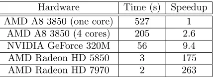
Hardware Time (s) Speedup AMD A8 3850 (one core) 527 1

AMD A8 3850 (4 cores) 205 2.6

NVIDIA GeForce 320M 56 9.4

AMD Radeon HD 5850 3 175

AMD Radeon HD 7970 2 263

Table 1. _{Simulations times on different hardware with single precisions. We observe}

interest-ing speedups for the GPU simulations compared to the one-core simulation. We also observe that OpenCL is still efficient on standard multicore CPU. The test case corresponds to the computation of300time steps of the algorithm on a1024×512grid. One numerical flux evalu-ation corresponds approximately to500 floating point operations (flop). Four flux evaluations are needed per cell and per time step. The amount of computations for this test is thus of the order of300Gflop.

• Computation of the CFL time step∆tn.We compute a local time step(∆tn)i,jon each cell and we use

a reduction algorithm(see [3]) in order to compute∆tn = min

i,j (∆tn)i,j.

• We perform the ALE-projection update inx-direction. We compute the fluxes balance in thex-direction for each cell of each row of the grid: a row or a part of a row is associated to one compute unit and one cell to one processor. As of October 2012, the OpenCL implementations generally impose a limit (typically 1024) for the number of work-items inside a work-group [8]. This forces us to split the rows for some large computations. The values in the cells are then loaded into the local cache memory of the compute unit. It is then possible to perform the ALE-projection algorithm with all the data into the cache memory in order to achieve the highest performance. The memory access is coalescent for reading and writing.

• We transpose the data matrix (exchange xandy) with an optimized memory transfer algorithm [16]. The optimized algorithm includes four steps:

– the data matrix is split into smaller tiles of size32×32. Each tile is associated to a compute unit,

– each tile is copied line by line from the global memory to the local memory of the compute unit. Memory access is coalescent because two successive processors read in two neighboring memory locations,

– we transpose each32×32tile in the local memory,

– each tile is copied line by line from the local memory to the global memory. The memory access is coalescent for writing.

• We perform the ALE-projection update iny-direction. The memory access is coalescent because of the previous transposition,

• We transpose again the data matrix for the next time step.

The repartition of the computational time on each kernel is the following: the ALE-projection steps represents

80%, the transposition11%and the time step computation9%of the global time computation.

We observe high efficiency (see Table 1) of the GPU implementation. The efficiency is explained by two important points.

• We used an optimized transposition algorithm to have coalescent access inxandydirections. Without this transposition, the computation would be10times slower.

d-c

GPU 1 GPU 2 GPU 3 GPU 4

Hôte

GPU l-1

GPU l

GPU l+1

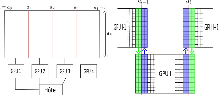
Figure 2. _{On the left: the computational domain is split into4subdomains. GPUlperforms}

the computations for the domain[al−1;al]×[c;d]. On the right: MPI transfers. Between each

iteration, GPUl has to exchange the values on the left and right boundaries with GPUsl−1

andl+1. On the picture we consider an overlap of2cells but for a second order implementation we need5cells.

3.2.

_MPI

The memory of a GPU is limited, typically to 1 gigabyte (GB), which limits us to a number of cells of the order of25,000,000. We will couple the parallelization on GPU (using OpenCL) with a subdomain paralleliza-tion, which uses the Message Passing Interface (MPI) standard. This allows a computation on several GPUs simultaneously. It will allow us to consider finer meshes and also reduce the computation time [1, 11, 13].

We use a standard subdomain decomposition, a GPU is associated to each subdomain. Thanks to MPI messages, we exchange the values at the subdomains boundaries. As we want a compatible decomposition with the matrix transpose algorithm, we split the initial domain only along the x-direction (see Figure 2). The exchanges between two GPUs will occur at each iteration. The GPU numberl will exchange information with GPUsl−1 andl+ 1.

Assume that we have a cluster of L GPUs and consider a two-dimensional computation on the domain

[a;b]×[c;d].We split the interval[a;b]as

a=a0< a1< a2<· · ·< aL=b,

withal=a+lb−_La,forl= 0,· · ·, L.

• the computational domain[al;al+1]×[c;d]is associated to the GPU numberl+ 1,

• each subdomain[al;al+1]×[c;d]is split into(Nx−gap)×Ny cells, wheregap∈ {2; 5} corresponds to

the number of cells in the overlap between subdomains.

– For a one-order computation, we usegap= 2cells in the overlap: one cell for the fluxes computa-tions and another one for the Glimm projection (8).

– For a second order computation, we use gap = 5 cells. Indeed, in the ALE step, we couple a MUSCL method to a Heun’s time integrator, then we need a two-cell overlap (one for the slopes of the MUSCL method and one for the flux) for each of the two steps of the Heun’s time integration. We need an additional one-cell overlap for the Glimm projection (8).

Grid 1 GPU 4 GPUs Speedup

2048×2048 14 s 14 s 1

4096×2048 22 s 16 s 1.4

4096×4096 77 s 60 s 1.3

8192×4096 150 s ? 61 s 2.5 16384×4096 600 s ? 230 s 2.6

Table 2. _{Simulations times for the MPI implementation on a cluster of4GPUs AMD Radeon}

HD7970. The computational domain is[0; 2]×[0; 1]. If the GPU is not fully occupied (meshes smaller than4096×4096), the computation times on one and on four GPUs are comparable. However if the GPU is fully occupied, for example for a grid of16384×4096, the MPI imple-mentation goes 2.6 times faster. This computation can not be done on only one GPU, thus some computation times are only estimated from a simple complexity analysis and marked by "?".

• we compute the stability condition. We compute the time step∆tl

n on each subdomainl and we take

∆tn= min 1≤l≤L∆t

l n.

• on each subdomain l= 1,· · · , L

– we associate a processor to each cell,

– we perform the time update underx-direction using the ALE- projection scheme,

– we transpose the data table,

– we perform they-direction update. For more details, see [12].

• We perform transfers between subdomains: each domainlsends thegapcolumns inside the left edge of the subdomain to the GPU numberl−1and thegapcolumns inside the right edge of the subdomain to the GPU numberl+ 1(see Figure 2). The GPU numberlreceives thegapcolumns from GPU number l−1 and thegapcolumns from GPU numberl+ 1(see Figure 2).

• On each subdomain l= 1,· · · , L, we transpose the data table so that the data are aligned in memory according to thex-direction for the next time step.

Remark 3.1. For MPI communications, we need firstly to copy data from each GPU to its host (CPU). Secondly we send MPI communications between hosts (CPUs). Finally, we copy data from CPU to GPU. As we perform the MPI communications before the data matrix transposition, memory access is coalescent for reading and writing.

The MPI implementation allows considering Ltimes finer mesh but is it faster? We test the method on a cluster of four AMD Radeon HD 7970 GPUs. The MPI communications represents globally 5% of the total time computation. The speedups are presented in the Table 2. The MPI implementation is faster with a factor

2.6.

4.

Numerical result

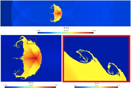
We now present a two-dimensional test that consists in simulating the impact of a Mach1.22shock traveling through air onto a (cylindrical) bubble of R22 gas. The shock speed is σ = 415m.s−1_{. This test aims at}

simulating the experiment of [9] and has been considered by several authors [14, 15, 18]. The initial conditions are depicted in Figure 3: a bubble ofR22is surrounded by air within aLx×Ly rectangular domain. Att= 0,

Shock

Post-shock

Pre-shock

R22 gas

r

y

x

Quantities Air (post-shock) Air (pre-shock) R22 ρ(kg.m−3_{) 1}

.686 1.225 3.863 u(m.s−1

) −113.5 0 0

v(m.s−1

) 0 0 0

p (Pa) 1.59×105 ₁

.01325×105 ₁

.01325×105

ϕ 0 0 1

γ 1.4 1.4 1.249

p∞ 0 0 0

Figure 3. _{Air-R22shock/cylinder interaction test. Description of the initial conditions on the}

left and initial data on the right.

planar shock is initially located atx=Lsand moves from right to left towards the bubble. The parameters for

this test are

Lx= 445mm, Ly= 89mm,Ls= 275mm,X1= 225mm,Y1= 44.5mm,r= 25mm.

BothR22and air are modeled by two perfect gases whose coefficientsγand initial states are given in the table of Figure 3.

The domain is discretized with a20 000×5 000regular mesh. Top and bottom boundary conditions are set to solid walls while we use constant state boundary conditions for the left and right boundaries. In Figure 4, we plot the densityρat the final timet1= 600µson the domain[0; 0.445]×[0; 0.089].The computation needs 3 hours on the four AMD Radeon HD 7970 GPUs cluster. The shocks are well resolved in the air and in the bubble. We can localize the position of the shock wave that impinges the bubble on the left side of the domain. On the second figure we zoom on the bubble. On the third one we zoom on the Rayleigh-Taylor instabilities that appears at the bubble interface. With a coarser mesh, we could not see these instabilities. For other pictures or for applications to liquid-gas flows, we refer to [10, 12].

5.

Conclusion

We have proposed a method for computing two-dimensional compressible flows with interface. Our approach is based on a robust relaxation Riemann solver, coupled with a very simple random choice sampling projection at the interface. The resulting scheme has properties that are not observed in other conservative schemes of the literature: it preserves velocity and pressure equilibrium at the two-fluid interface, it is conservative in mean, it does not diffuse the mass fractionϕ, it preserves the non convex hyperbolic domainH.

In addition, the algorithm is easy to parallelize on recent multicore architectures. We have implemented the scheme in the OpenCL environment. Compared to a standard CPU implementation, we observed that the GPU computations are more than hundred times faster. This factor is essentially due to the optimized transposition that we perform betweenxandy update and to the relaxation solver that gives a robust but simple expression of the numerical fluxes. As the computation is very fast, the limiting factor becomes the memory size of a GPU. The MPI version permits to treat very fine meshes. We test the code on R22/Air shock bubble interaction, thanks to a very fine mesh we can observe Rayleigh-Taylor instabilities at the bubble interface.

References

[1] D. Aubert and R. Teyssier. Reionization simulations powered by graphics processing units. i. on the structure of the ultraviolet radiation field.The Astrophysical Journal, 724:244–266, 2010.

[2] M. Bachmann, P. Helluy, J. Jung, H. Mathis, and S. Müller. Random sampling remap for compressible two-phase flows. Computers and Fluids, 86:275–283, 2013.

[3] G.E. Blelloch. Scans as primitive parallel operations.IEEE Transactions on Computers, 38(11):1526–1538, 1989.

Figure 4. _{Density at final timet1= 600µs. On the first picture we represent all the domain,}

on the second one we do a zoom on the bubble and on the third we zoom on the Rayleigh-Taylor instability. On this picture, we can observe the precision of the computation.

[5] C. Chalons and F. Coquel. Computing material fronts with a lagrange-projection approach.HYP2010 Proc.,http://hal. archives-ouvertes.fr/docs/00/54/89/38/PDF/chalons_coquel_hyp2010.pdf, 2010.

[6] C. Chalons and P. Goatin. Godunov scheme and sampling technique for computing phase transitions in traffic flow modeling. Interfaces and Free Boundaries, 10(2):197–221, 2008.

[7] P. Colella. Glimm’s method for gas dynamics.SIAM, J. Sci. Stat. Comput., 3(1), 1982. [8] Khronos Group. Opencl online documentation.http://www.khronos.org/opencl/.

[9] J. F. Haas and B Sturtevant. Interaction of weak shock waves with cylindrical ans spherical gas inhomogeneities.J. Fluid Mechanics, 181:41–71, 1987.

[10] P. Helluy and J. Jung. Opencl simulations of two-fluid compressible flows with a random choice method.IJFV International Journal On Finite Volumes, 10:1–38, 2013.

[11] D. A. Jacobsen, J.-C. Thibault, and I Senocak. An mpi-cuda implementation for massively parallel incompressible flow com-putations on multi-gpu clusters.48th AIAA Aerospace Sciences Meeting and Exhibit, 2010.

[12] J. Jung.Schémas numériques adaptés aux accélérateurs multicoeurs pour les écoulements bifluides. PhD thesis, University of Strasbourg, 2013.

[13] V. V. Kindratenko, J. Enos, M. T. Showerman, G. W. Arnold, J. E. Stone, J. C. Phillips, and W.-M. Hwu. Gpu clusters for high- performance computing.Proc. Workshop on Parallel Programming on Accelerator Clusters, IEEE Cluster 2009, pages 1–8, 2009.

[14] S. Kokh and F. Lagoutière. An anti-diffusive numerical scheme for the simulation of interfaces between compressible fluids by means of the five-equation model.J. Computational Physics, 229:2773–2809, 2010.

[15] J. J. Quirk and S. Karni. On the dynamics of a shock-bubble interaction.J. Fluid Mechanics, 318:129–163, 1996. [16] G. Ruetsch and P. Micikevicius. Optimizing matrix transpose in cuda.NVIDIA GPU Computing SDK, pages 1–24, 2009. [17] R. Saurel and R. Abgrall. A simple method for compressible multifluid flows.SIAM J. Sci. Comput., 21(3):1115–1145, 1999. [18] K. M. Shyue. A wave-propagation based volume tracking method for compressible multicomponent flow in two space