https://doi.org/10.5194/gmd-12-785-2019 © Author(s) 2019. This work is distributed under the Creative Commons Attribution 4.0 License.
The Air-temperature Response to Green/blue-infrastructure
Evaluation Tool (TARGET v1.0): an efficient and
user-friendly model of city cooling
Ashley M. Broadbent1,2,3,4, Andrew M. Coutts3,4, Kerry A. Nice3,4,5, Matthias Demuzere6,7, E. Scott Krayenhoff8,1,2, Nigel J. Tapper3,4, and Hendrik Wouters7,6
1School of Geographical Sciences and Urban Planning, Arizona State University, Tempe, Arizona, USA 2Urban Climate Research Center, Arizona State University, Tempe, Arizona, USA
3School of Earth, Atmosphere and Environment, Monash University, Clayton, Australia 4Cooperative Research Centre for Water Sensitive Cities, Melbourne, Australia
5Transport, Health, and Urban Design Hub, Faculty of Architecture, Building, and Planning,
University of Melbourne, Melbourne, Victoria, Australia
6Ghent University, Laboratory of Hydrology and Water Management, Ghent, Belgium
7KU Leuven, Department of Earth and Environmental Sciences, Celestijnenlaan, Leuven, Belgium 8School of Environmental Sciences, University of Guelph, Guelph, Ontario, Canada
Correspondence:Ashley M. Broadbent ([email protected]) Received: 12 July 2018 – Discussion started: 8 October 2018
Revised: 3 February 2019 – Accepted: 4 February 2019 – Published: 20 February 2019
Abstract. The adverse impacts of urban heat and global climate change are leading policymakers to consider green and blue infrastructure (GBI) for heat mitigation benefits. Though many models exist to evaluate the cooling impacts of GBI, their complexity and computational demand leaves most of them largely inaccessible to those without specialist expertise and computing facilities. Here a new model called The Air-temperature Response to Green/blue-infrastructure Evaluation Tool (TARGET) is presented. TARGET is de-signed to be efficient and easy to use, with fewer user-defined parameters and less model input data required than other urban climate models. TARGET can be used to model av-erage street-level air temperature at canyon-to-block scales (e.g. 100 m resolution), meaning it can be used to assess tem-perature impacts of suburb-to-city-scale GBI proposals. The model aims to balance realistic representation of physical processes and computation efficiency. An evaluation against two different datasets shows that TARGET can reproduce the magnitude and patterns of both air temperature and surface temperature within suburban environments. To demonstrate the utility of the model for planners and policymakers, the results from two precinct-scale heat mitigation scenarios are presented. TARGET is available to the public, and ongoing
development, including a graphical user interface, is planned for future work.
1 Introduction
unsubstan-tiated estimates of cooling magnitudes. Consequently, there is a need for simple, computationally efficient, and scientif-ically defensible urban climate models that can be used by consultants to provide reliable estimates of cooling to gov-ernmental planners and policymakers.
There are a number of existing micro-to-local-scale ur-ban models capable of modelling GBI. The most complex models are primarily based on computational fluid dynam-ics (CFD) techniques. These include ENVI-met, hand-coded CFD models (such as OpenFOAM; OpenFOAM, 2011; or STAR-CD; CD-adapco, 2011) and other CFD-based ap-proaches (Bailey et al., 2014, 2016; Kunz et al., 2000; Schlünzen et al., 2011; Yamada and Koike, 2011; Bruse, 1999). ENVI-met is the most commonly used urban mi-croclimate model. However, numerous ENVI-met studies have reported concerns with model accuracy, particularly for representation of vegetation (Ali-Toudert and Mayer, 2006; Krüger et al., 2011; Acero and Herranz-Pascual, 2015; Span-genberg et al., 2008). In addition, the complexity of configu-ration and computational intensity of all CFD-based models (i.e. 24 h of simulation requiring 24 h of computation time) puts their usage out of the reach of non-specialized users.
A second group of commonly used models, such as SOL-WEIG (Lindberg et al., 2008) and RayMan (Matzarakis et al., 2007, 2010), focus on radiation fluxes in urban areas. These models have been used to assess GBI cooling, espe-cially tree shading. However, the limitations of these models may not allow a complete assessment of GBI cooling because the effects of evapotranspiration are neglected. The Temper-atures of Urban Facets in 3-D (TUF-3D) model (Krayen-hoff and Voogt, 2007) and a vegetated derivative (VTUF-3D) (Nice et al., 2018) provide a precise representation of urban canyon physical processes. However, TUF-3D and VTUF-3D require a high level of computer power, modelling expe-rience, and parameter set-up.
The canyon air temperature (CAT) model (Erell and Williamson, 2006) shows potential as a computationally ef-ficient model that calculates air temperatures using urban building and vegetation geometry and moisture availability. However, the lack of surface temperature prediction makes it difficult to derive human thermal comfort indexes. The Town Energy Balance (TEB) model (Masson, 2000) has emerged as a popular urban area parameterization scheme. The TEB-Veg (Lemonsu et al., 2012; Redon et al., 2017) variation in-cludes urban vegetation and provides functionality to assess cooling impacts of GBI. However, the TEB-Veg model con-figuration and application requires a level of modelling skill normally outside the capability of environmental consultants. While not an air temperature model, the Local-Scale Urban Meteorological Parameterization Scheme (LUMPS) (Grimmond and Oke, 2002) has been widely used to assess the impacts of GBI on surface energy balance (SEB). The Surface Urban Energy and Water Balance Scheme (SUEWS) (Järvi et al., 2011), a superset of LUMPS with added ur-ban water balance functionality, provides a means to assess
vegetation (and associated soil) transpiration impacts at local scales. SUEWS shows good performance in SEB evaluations for Vancouver and Los Angeles (Järvi et al., 2011), Helsinki (Järvi et al., 2014), and Singapore (Demuzere et al., 2017). Due to the success and simplicity of LUMPS, we use it as a key component of the model presented here.
The lack of an efficient yet accessible tool for assess-ing GBI is identified as a research gap. Here we introduce and evaluate a new model called The Air-temperature Re-sponse to Green/blue-infrastructure Evaluation Tool (TAR-GET). TARGET is a simple modelling tool that calculates surface temperature and street-level (below roof height) air temperature in urban areas. TARGET is designed to make quick and accurate assessments of urban temperatures and GBI cooling impacts with minimal input data requirements. TARGET calculates the average air temperature at street level in urban areas but does not represent micro-scale vari-ations of radiation exchange or wind flow at the human scale. The model is designed to be used at the urban canyon to block scales (100–500 m). We recommend a minimum spatial resolution of 100 m for air temperature simulations and 30 m for surface temperature. It can be used to as-sess the canyon-averaged impacts of street-scale interven-tions or larger-scale suburban greening projects. TARGET is a climate-service-oriented tool that provides a first-order approximation of the impacts of GBI on surface temperature and street-level air temperature to provide scientific guidance to practitioners during the planning process. The computa-tional efficiency of the model is such that a user (with 1–2 h of training) can calculate in minutes the 100 m horizontal res-olution cooling effects, on a normal desktop computer, across an entire suburb/local government area or neighbourhood.
The main aims of this paper are the following: (1) to pro-vide a technical description of TARGET, (2) to propro-vide de-tailed evaluation of model performance, and (3) to provide proof of concept and illustrate how the model can be opera-tionalized by consultants and practitioners.
2 Model description 2.1 Model overview
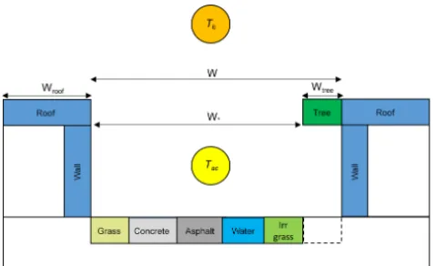
As outlined in Fig. 1, TARGET treats each model grid point as an idealized urban canyon with roofs, walls, and ground-level facets. Roof width (Wroof), building height (H), tree
width (Wtree), and street width (W) are used to define the
Figure 1. Schematic of TARGET urban canyon set-up.Tacis the canopy layer air temperature, andTbis the above-canopy air tem-perature, which is a uniform value across the whole domain.Wroof is the roof width,Wtreeis the tree width,W is canyon width, and W∗ =W−Wtree. The surface beneath trees is assumed to be repre-sentative of canyon ground-level surfaces.
Fig. 1, the width of the canyon (and therefore the amount of radiation that enters and leaves the canyon) is modulated by the planar area of trees. The simple method implies that none of the radiation effectively “intercepted” by trees enters the canyon. The area underneath trees (not shown in planar land cover maps) is added to the model to represent the additional thermal mass. This simple approach allows for a first-order representation of two major process associated with trees: so-lar shading and longwave trapping.
Additionally, water bodies are treated separate to all other surfaces using an independent module. More details about the model process are shown in Fig. 2. For each grid point, the average surface characteristics are used to calculate an aggregated surface temperature (Tsurf).Tsurfis converted to
an average canopy layer air temperature (Tac) using an
esti-mated canopy wind speed (Ucan) and above-canopy air
tem-perature (Tb). A uniformTbfor all grid points is diagnosed
for each time step using reference meteorological variables. 2.2 Input data requirements
2.2.1 Land cover
TARGET uses simple data inputs that are intended to be eas-ily accessible. The model requires the user to define the plan area of buildings (Aroof), concrete (Aconc), asphalt (Aasph),
grass (Agras), irrigated grass (Aigrs), tree (Atree), and water
(Awatr). These land cover categories are self-explanatory and
describe most of the surfaces present in urban areas. Lo-cal governments often have geographiLo-cal information system (GIS) datasets of land cover and/or land use that can be used for land cover input data. Further, we intend to develop a graphical user interface (GUI) that allows users to easily in-put land cover datasets and define the model domain. This feature will allow users to convert and upload GIS data (e.g.
Figure 2.Overview of approach used in TARGET.Tacis street-level (urban canopy layer) air temperature (◦C),Tbis the air tem-perature above the urban canopy layer (◦C),Tsurf,i is the surface
temperature for surface typei,K↓is incoming shortwave radiation (W m−2),L↓is incoming longwave radiation (W m−2),Tais ref-erence air temperature (◦C),Rnis net radiation (W m−2), RH is rel-ative humidity (%),Fiis the fraction of land cover typei(%),QH,i
is the sensible heat flux for surfaceifrom LUMPS (W m−2),QG,i
is the storage heat flux for surface typeifrom LUMPS (W m−2), Uzis the reference wind speed (m s−1),H is the average building
height (m),W is the average street width (m),rs is the resistance from the surface to the canopy (s m−1), andra is the resistance from urban canopy to the atmosphere (s m−1).Tb∗ is a homoge-neous value for the whole domain, which is diagnosed through the processes laid out in Sect. 2.7.
shape and raster files) directly into the model. The Wroof, Wtree,W,W∗, and wall area (Awall) are calculated from plan
area land cover inputs. However, average building height (m) must be user-defined or set to a domain average value. If tailed land cover data are not available, input data can be de-fined from existing land-use lookup tables or from databases such as the World Urban Database and Portal Tool (WU-DAPT) (Mills et al., 2015; Ching et al., 2018). See Wouters et al. (2016) for an example of how the WUDAPT data could be integrated.
2.2.2 Meteorological data
TARGET requires reference meteorological data to drive the model and calculate street-level air temperature. The follow-ing meteorological variables are required: incomfollow-ing short-wave (solar) radiation (K↓), incoming longwave (terres-trial) radiation (L↓), relative humidity (RH), reference wind speed (typically at 10 m) (Uz), and air temperature (Ta). The
user must define the height above ground of reference Uz andTa. Meteorological data should be representative of a
2.3 Radiation calculation
The net radiation of theith surface type (Rn,i) is calculated using the following:
Rn,i =
K↓(1−αi)+i
L↓ −σ Tsurf4 ,i,[t−2]SVFi, (1)
where αi is surface albedo, i is surface emissivity, andσ is the Stefan–Boltzmann constant (5.67×10⁻⁸W m−2K−4). Theαi andivalues are predefined for each surface (see Ta-ble 1). The right-hand side of the equation accounts for net longwave radiation. The modelledTsurf,i,[t−2]from two time
steps(t )previously is used to calculateL↑. This is neces-sary to avoid circular logic in model calculations; modelled
Tsurf,i,[t−2]is calculated using the storage heat flux (QG,i), which takes Rn from the previous time step. The time lag
does not significantly affect calculations when a 30 min time step is used. The average sky view factor (SVFi) is included to broadly represent the interception of incoming and outgo-ing short- and longwave radiation by buildoutgo-ings and trees on the radiation balance. Addition of SVF restricts the net radi-ation exchange of each facet to its total view factor occupied by sky. It assumes that walls and ground surfaces have sim-ilar longwave emission relative to the sky and that the solar radiation receipt can be approximated by SVF, on average. This simplification means that the model makes no distinc-tion between lit and unlit buildings walls and roads. SVFifor ground-level, wall, and roof facets is defined as (Sparrow and Cess, 1978)
SVFground=
" 1+ H W∗ 2# 1 2 − H
W∗; (2)
SVFwall=
1 2
1+
W∗ H − " 1+ W∗ H 2# 1 2
; (3)
SVFroof=1. (4)
The Rn,i is then used to calculate aQG,i for each surface type.
2.4 Storage heat flux (QG) calculation
The storage heat flux (QG,i) for theith land cover class is calculated using an adapted version of the objective hystere-sis model (OHM) (Grimmond and Oke, 2002):
QG,i=Rn,ia1,i+
∂R
n,i
∂t
a2,i+a3,i, (5)
where ∂Rn,i
∂t =0.5(Rn,i,(t−1)−Rn,i,(t+1))and the threea co-efficients are defined using cited values for each surface (see Table 1). The a coefficients capture the hysteresis pattern commonly observed between theRnandQG,i in urban ar-eas. See Grimmond and Oke (1999) for a full description of
the OHM and the role of thea parameters inQG,i calcula-tions. The QG,i is then used to calculate theTsurf for each
land cover type using the “force–restore” method. 2.5 Surface temperature calculation (force–restore) The force–restore method is an efficient method for cal-culating surface temperature (Bhumralkar, 1975; Deardorff, 1978) and is an alternative to multilayer conduction ap-proaches used in other climate models. The force–restore method is used to ensure that the model remains computa-tionally efficient. The ground layer is conceptually divided into two layers with uniform vertical temperature: a thin sur-face layer and a deep soil layer. The forcing term, which is driven by QG,i, heats the surface layer. The restore term, driven by deep soil temperature, dampens the forcing term. The change in surface temperatureTsurf for surfacei, with
respect to time(t ), is calculated as (Jacobs et al., 2000)
∂Tsurf,i
∂t =
QG,i
CiD
−2π
τ (Tsurf,i,[t−1]−Tm,i,[t−1]), (6)
whereCi is the volumetric heat capacity (J m−3K−1),τ is the period (86 400 s), D is the damping depth of the diur-nal temperature waveD=2κ/ω0.5,ω=2π/τ, andκ repre-sents thermal diffusivity. The average soil (ground) tempera-ture (◦C) (T
m) is calculated using
∂Tm,i
∂t =
1QG,i
CiDy
, (7)
whereDy=D √
365, the damping depth for the annual tem-perature cycle (m).
The force–restore method, which assumes two layers each of uniform temperature, cannot be applied to more complex surfaces such as water, trees, walls, or roofs. For roofs we set
C at a realistic value and useκ as a tuning parameter to rep-resent layers of thermally active mass characteristic of most building roofs, which are often thinner than ground-level sur-faces. This approach produces accurateTsurf,roofresults (see
Sect. 3.2), but ongoing work is needed to represent roofs in a physically realistic and efficient manner. For simplicity, the wall surfaces are assumed to have the same thermal proper-ties as roofs. For trees, we assume thatTsurf,treeis equal toTa
(see Fig. B3 for justification), and a simple water body model is used to calculateTsurf,watr.
2.6 Simple water body model
The water model is used for modelling small inland wa-ter bodies, such as lakes and wetlands. Our analysis sug-gests that the OHM–force–restore method cannot be used to reliably reproduce water surface temperatures. We tested the OHM modifications and parameters used by Ward et al. (2016) and found substantial over-predictions of surface wa-ter temperature (over 10◦C) during the day. As such, we de-veloped a simple water body model to stand in for the OHM– force–restore method. The water model in TARGET is based
on a single water layer, overlaying a soil layer. Essentially, the force–restore surface temperature model is implemented and is overlain by a homogeneous mixed water layer (i.e. ne-glecting thermal stratification) representing a water body of depthdwatr(m). The model is designed to apply to water
bod-ies of 0.1–1.0 m depths. The water model is based on the pan evaporation model of Molina Martínez et al. (2006), which closely follows that of the lake model of Jacobs et al. (1998). The water body model also determines the surface energy balance of the water surface. The energy balance model for the water layer is given by Molina Martínez et al. (2006):
Sab+Ln+QH,watr−QE,watr−QG,watr−1QS,watr=0, (8)
whereSab is absorbed shortwave radiation (W m−2),Ln is
the net longwave radiation (W m−2),QG,watris the
convec-tive heat flux at the bottom of the water layer and into the soil below (W m−2), and1QS,watris the change in heat
stor-age of the water layer (W m−2). Solar radiation penetrates the water surface and is absorbed as described by Beer’s law (Molina Martínez et al., 2006):
Sab=Knβk+(1−βk)(1−e−η), (9)
whereKnis the net shortwave radiation (W m−2),βk is the amount of shortwave radiation immediately absorbed by the water layer (set to 0.45) (Molina Martínez et al., 2006), andη
is the extinction coefficient. Here,ηis calculated according to Subin et al. (2012), for the water layer with depthdwatr
(m):
η=1.1925dwatr−0.424. (10)
A correction factor for the solar path length zenith angle is often applied to Eq. (9) (Molina Martínez et al., 2006), but this is omitted from TARGET to reduce complexity.
TheQG,watrinto the soil at the base of the water layer is
given by Molina Martínez et al. (2006):
QG,watr= −Cwatrκwatr
1T
1dwatr
, (11)
where Cwatr is the volumetric heat capacity of water
(4.18×10⁶J m−3K−1),κwatris the eddy diffusivity of
wa-ter (m2s−1), and the change in depth is1dwatr=dwatr (the
depth of the water layer).κwatris a complex function
account-ing for thermal stratification of water and surface friction velocity. To reduce complexity, and assuming a mixed ho-mogeneous water layer, a constantκwatris selected based on
shallow lakes reported in Salas De León et al. (2016). The change in temperature1T (◦C) is the difference between the water temperatureTsurf,watr(◦C) and the soil temperature
be-neath the water layerTsoil (◦C).Tsoil is calculated using the
Eq. (6): dTsoil
dt =
QG,watr+(Kn−Sab)
CwatrD
−2π
τ Tsoil,[t−1]−Tm,[t−1]
. (12)
To represent the radiation that is not absorbed by the water but is absorbed by the underlying soil layer,Kn−Sabis added
toQG,watr.
The latent heat flux (QE,watr) (W m−2) is given by Arya
(2001):
QE,watr=ρvLvhvUz(qs−qa) , (13)
whereρvis the density of moist air (kg m−3),Lv is the
la-tent heat of vaporization (i.e. 2.43 MJ kg−1),hvis the bulk
transfer coefficient for moisture (1.4×10⁻³)(Hicks, 1972; Jones et al., 2005),Uzis the reference wind speed,qsis the
saturated specific humidity atTsurf,watr, andqais the specific
humidity of the air for the givenTa.
The sensible heat flux above the water surface is given by Molina Martínez et al. (2006):
QH,watr=ρaCphcUz Ta−Tsurf,watr, (14)
whereρais the density of dry air (=1.2 kg m−3),Cpthe spe-cific heat of air (1013 J kg−1K−1), andhc the bulk transfer
coefficient for heat (hc=hv).
Returning to Eq. (9), net long wave radiationLn=Rn− Kn, leaving 1QS,watr from the energy balance equation,
which is defined as (Molina Martínez et al., 2006)
1QS,watr=Cwatrdwatr
1Tsurf,watr
1t , (15)
where1t is change in time (s), andCwatr is the volumetric
heat capacity of water (J m−2K−1). Solving for 1Tsurf,watr
and adding the change in temperature to the previous time step (Tsurf,watr[t+1]=Tsurf,watr,[t]+1Tsurf,watr) gives the new
water layer temperature.
2.7 Calculation of urban canopy layer air temperature (Tac)
To calculateTacwe first calculate a domainTbfor each time
step. Assuming air temperature at 3 times the building height (3H) is consistent between the neighbourhood of interest and the reference weather station location, we extrapolate refer-ence air temperature at measurement height to 3H assuming a constant flux layer and using a bulk Richardson-number-based approximation (Mascart et al., 1995). Through this simple calculation we define a domain constantTbwith the
basic representation of atmospheric stability in TARGET. The canyon air temperature is then calculated using a mod-ified version of the canopy air temperature equation from
the Community Land Model Urban (CLMU) (Oleson et al., 2010):
Tac=
7
P
i
Tsurf,icsFi+
"
Tsurf,roof
1 cs+
1 ca
Froof
#
+(TbcaW )
7
P
i
(csFi)+
"
Froof
1 cs+
1 ca
#
+(caW )
, (16)
whereFiandTsurf,iare the 2-D fractional coverage and sur-face temperature of sursur-faceiin the canyon,csis the
conduc-tance from the surface to the urban canopy layer (m s−1), and ca is the conductance from the urban canopy to the
above-canopy surface layer (m s−1). In Eq. (16) we assume roofs are connected to the canyon via two resistances in series, thus representing the additional impediment to the transfer of heat from a rooftop into the canyon. We hypothesize that the heat transfer from roofs to the canyon air can be approximated by two resistances in series (the canyon-to-atmosphere re-sistance,ca, and surface-to-canyon resistance,cs). The logic
here is that resistance to heat transfer from the roof surface to the canyon should be greater thancaorcs independently.
Through sensitivity testing we are able to demonstrate that this assumption improves predicted canyon air temperature. Thecais calculated following Masson (2000) and using the
stability coefficients from Mascart et al. (1995). Thecsterm
is from Masson (2000):
rs=
ρaCp
11.8+4.2Ucan
, (17)
where cs=rs1 and Ucan is the wind speed in the canyon
(m s−1) (Kusaka et al., 2001):
Ucan=Utopexp
−0.386H
W
, (18)
whereUtopis the wind speed at the top of the canyon (m s−1). Utopis estimated at 3H based on the observed wind speed at
a nearby observational site (ideally an airport) using a loga-rithmic relationship. Airports are relatively devoid of rough-ness elements, and wind speed is typically measured at 10 m above the surface. As such, the assumption of a logarithmic profile through the roughness sublayer (Masson, 2000) is im-posed.
3 Methods and data 3.1 Overview
As part of the model evaluation, we conduct a range of sim-ulations that test model performance for bothTsurfandTac.
each land cover type that can be prescribed in TARGET (i.e. dry grass, asphalt etc.), using ground-based observations of
Tsurf(Sect. 3.2). These simulations by land cover type
pro-vide a detailed assessment of model parameters and the un-derlying energy balance dynamics and resultingTsurffor each
land cover class. Second, we conduct suburb-scale simula-tions of Mawson Lakes, Adelaide, for which we have high-resolution remotely sensedTsurfobservations and in situTac
data (Sect. 3.3). The suburb-scale simulations reflect the way the model is intended to be used by practitioners.
3.2 Land cover simulations
To test model performance at simulating Tsurf of different
land cover classes and perform sensitivity analysis on a number of model parameters, we use ground-based observa-tions ofTsurffrom the Melbourne metropolitan area. Coutts
et al. (2016) deployed infrared temperature sensors (SI-121, Apogee), during February 2012 (5 min averages), across a range of land cover types including asphalt, concrete, grass, irrigated grass, steel roof, and water. Infrared sensors were mounted above the aforementioned surface types installed at heights of approximately 1.5–2 m. The conditions dur-ing this period represented near-typical summertime condi-tions in Melbourne, including a number of days (15, 24, and 25 February) when air temperature exceeded 30◦C (see Fig. B1). These hotter days were characterized by northerly winds, which bring hot and dry air from Australia’s interior and often result in heatwave conditions in Melbourne. Ad-ditionally, there was at least one cloudy day when incoming shortwave radiation (K↓) dropped significantly and a neg-ligible amount of rainfall occurred (17 February). To com-pare the Coutts et al. (2016) observations with TARGET we run the model for each surface type (i.e. 100 % grass or roof etc.) with radiation forcing data from the Melbourne Airport weather station during the time period in question. TheTb
calculation is not needed since we only calculated Tsurffor
this part of the model evaluation. The 30 min output from TARGET is compared withTsurfobservations, and statistics
are calculated.
3.3 Suburb-scale simulations (Mawson Lakes)
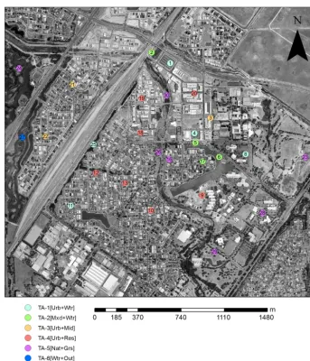
In addition to the land cover category testing, we also con-duct suburb-scale simulations of Tsurf and Tac for
Maw-son Lakes, Adelaide (Fig. 3). The suburb-scale simulations use observational data from the Mawson Lakes field cam-paign, conducted during 13–18 February 2011, which repre-sented average summertime conditions in Adelaide (Broad-bent et al., 2018b). For these simulations, the model is run on 30 m (Tsurf) and 100 m (Tac) grids over the Mawson Lakes
suburb for the period 13–18 February (Fig. B2). Remotely sensed land cover data from the campaign are used to define land cover, and building morphology is defined using lidar data (see Broadbent et al., 2018b). The Mawson Lakes
simu-lations use the same parameter set-up as above (summarized in Table 1) and are forced with meteorological data from the Kent Town Bureau of Meteorology (ID 023090) weather station. ModelledTsurfis validated using observed remotely
sensedTsurf (night – 15 February and day – 16 February),
which is resampled to 30 m resolution (Broadbent et al., 2018b). To validate Tac, we use data from 27 automatic
weather stations (AWSs) that were also deployed during the Mawson Lakes field campaign (see Fig. 3 for AWS loca-tions).
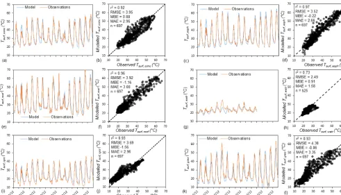
4 Model evaluation results and discussion 4.1 Land cover simulations
The surface temperature for each land cover class is simu-lated for a 14-day period during February 2012. The results show that modelled surface temperature for all three impervi-ous surfaces (concrete, asphalt, and roof) is reasonably well predicted, with a mean bias error (MBE) of 0.88,−0.22, and −1.16◦C, respectively (Fig. 4a–f). The root mean square er-ror (RMSE) values for impervious surfaces are around 3.5– 4◦C. These RMSE values represent about 15 % of diurnal
Tsurfvariation, which implies good model skill given the
sim-plicity of the approach.
The night of the 16 February is not well captured at the concrete and asphalt sites. The Tsurf,conc andTsurf,asph are
under-predicted (up to 5◦C cooler than observations) on the night of 16 February, which may have been caused by warm air advection. The TARGET approach cannot account for the effects of warm air advection on surface temperature, as there is no feedback betweenTacandTsurf. Despite this limitation,
the broad timing and magnitude of heating and cooling are well captured for all three impervious land cover types.
Model performance for Tsurf,watr had a low MBE of
0.91◦C, but ther2value of 0.76 suggests the model captured diurnalTsurf,watrvariation less accurately than other surfaces
(Fig. 4g–h). In particular, daily maximumTsurf,watrvalues are
under-predicted on hotter days (e.g. 14 February). TARGET uses a different module for water bodies (see Sect. 2.6). This simple module treats water as a single layer overlying soil. Despite the under-prediction on 14 February, the simple wa-ter body model can reproduceTsurf,watrto an acceptable
stan-dard.
Modelled Tsurf,irgs had a MBE (−1.56◦C) comparable
to that of impervious surfaces (Fig. 4i–j). However, the RMSE for irrigated grass (3.69◦C) represents approximately
20 % of diurnal Tsurf,igrs variation, suggesting model error
is slightly higher than for the impervious surfaces. Gener-ally Tsurf,igrs is slightly over-predicted at night and
Figure 3.Mawson Lakes suburb with weather station locations. The numbers indicate individual weather stations, while the colour cod-ing specifies groups of sites with statistically similar thermal characteristics. The names of each cluster indicate the average land sur-face characteristics: urban sites with nearby water (TA-1[Urb+Wtr]), mixed land use with nearby water (TA-2[Mxd+Wtr]), urban
mid-rise-type sites (TA-3[Urb+Mid]), urban residential sites (TA-4[Urb+Res]), natural grass-dominated sites (TA-5[Nat+Grs]), and a single outlier site
(TA-6[outlier]) (Broadbent et al., 2018b).
Dry grass had a small MBE (0.06◦C) but the largest RMSE of the surfaces tested (4.38◦C). However, this RMSE only equated to approximately 10 %–15 % of diurnal
Tsurf,gras variability (Fig. 4k–l) as dry grass had the largest
amplitude of surface temperature variability. Dry grass ex-hibited the same skewing in the scatter plot as irrigated grass, with a general over-prediction of night-time temperatures and under-prediction of daytime maxima.
4.2 Suburb-scale simulations (Mawson Lakes) 4.2.1 Surface temperature
In addition to the land cover simulations, we conduct suburb-scale modelling of the Mawson Lakes site. These
simula-tions reveal how the TARGET model can be operationalized by practitioners who want to assess the cooling benefits of blue infrastructure or greening initiatives. Suburb-scale sim-ulations are conducted using the same parameters as above (Table 1). We run the model at 30 m spatial resolution for
Tsurfsimulations and 100 m for simulations ofTac. Figure 5
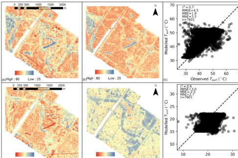
shows the predictedTsurffor the Mawson Lakes domain
plot-ted against observedTsurf. The Mawson Lakes simulations
revealed the initial conditions of the Tm parameter (which
represents the average temperature in the ground layer) are important for good model performance. A spin-up period (1 month) had to be used to obtain initialTmvalues for each
sur-Figure 4.Observed vs. modelled(a, b)Tsurf,conc,(c, d)Tsurf,asph,(e, f)Tsurf,roof,(g, h)Tsurf,watr,(i, j)Tsurf,irgs, and(k, l)Tsurf,gras. All time series plots are for the period 11–25 February. Note that the water site only had observational data for the period 11–21 February due to instrument failure;r2is the correlation coefficient, RMSE is the root mean square error, MBE is the mean bias error, and MAE is the mean absolute error.
face type. A future version of the model will automatically spin up initialTmvalues. The model output also shows that
some of the input land cover is poorly categorized, result-ing in the population of grid points in which modelledTsurf
is over-predicted. Additionally, errors in the observed Tsurf
caused by heterogeneity of roof emissivity also contribute to apparent inaccuracies of modelledTsurf. In general, the
day-time Tsurf is slightly over-predicted, and the complexity of
spatial variability is not fully captured. However, this is a positive result given that only eight land cover classes are represented in the model. Overall, the daytime Tsurfis well
predicted, with the range and magnitude ofTsurfcaptured by
the model.
The results suggest that night-timeTsurfis under-predicted
by model. The range of modelled nocturnal Tsurf
variabil-ity (8◦C) is much smaller than observed variability (18◦C). This under-prediction of variability could reflect the fact that some processes that dictate the rate of nocturnal cooling are not fully accounted for in this approach. Nevertheless, the general spatial patterns of Tsurf are captured well. Further,
given that the range of Tsurf is smaller at night, this
under-prediction is of minimal consequence for modelledTac. The
nocturnalTsurfof impervious surfaces is also under-predicted
in the land cover simulations (i.e. Sect. 4.1) under warm advection conditions. Although warm advection conditions
were not observed during the Mawson Lakes campaign, it is worthwhile further investigating this phenomenon in future work to negate its effect and improve nocturnalTsurf
accu-racy.
4.2.2 Air temperature
Spatial plots of modelled 03:00 and 15:00Tacare shown in
Fig. 6. The modelled air temperatures are biased towards warmer air temperature in urban areas and cooler air tem-perature in rural areas. These biases are partly driven by the lack of advection in the model. Without atmospheric mixing, the local impacts of pervious and impervious surfaces are ex-aggerated, causing an additional cooling and warming effect in rural and urban areas, respectively However, the general patterns ofTac are reasonable and as expected. We also
ex-tract modelledTacfrom the grid points where the 27 AWSs
are located (grid points were centred at the AWS) for a 2-day period (15–16 February 2011) (Fig. 7). TheTacis generally
Figure 5.Mawson Lakes observed(a, d)Tsurfand modelled(b, e)Tsurffor day(a–c)and night(d–e). Areas where land cover is categorized as “other” are not simulated. Note that Tsurf here does not includeTsurf,wall for comparison with horizontally averaged aerial imagery observations.
Figure 7.ModelledTacvs. observedTacfor Mawson Lakes weather stations (15–16 February 2011, 30 min data). The numbers and colours correspond to individual stations and clusters shown in Fig. 3.
Additionally, TARGET does not require the user to provide above-canyon forcing data (e.g. Tb), which are needed for
other models and are not easily obtained. TARGET tends to over-predict averageTacat all urban sites (Fig. 8).
Residen-tial sites (TA-4[Urb+Res] cluster [red]) are too warm during
the day. This over-prediction is likely due to the uniform wall and roof thermal parameters used, which are not representa-tive of residential areas. Further, the lack of horizontal mix-ing may have exacerbated warmer temperatures in these ar-eas. By contrast, the TA-5[Nat+Grs]cluster is too cool at night.
The model predicts the formation of a stable layer with cool air trapped near the surface. Overall, the diurnal range and averageTacare well captured by the model.
Finally, there is some hysteresis in Fig. 6, indicating that modelledTacis slightly out of sync with observedTac. This
could be due to the approach used to diagnoseTb, which
as-sumes a constantRiin the surface layer and therefore heats up too quickly during the morning. Improvement in theTb
term is an area for future model development. However, we believe it is important that TARGET calculates Tb, as
this makes the model much more accessible to non-expert users. Given the simplicity and computational efficiency of the model approaches used, TARGET shows good skill for predicting urbanTac. Overall, the air temperature evaluation
shows we can have confidence in the accuracy of the model and its potential to be used by practitioners.
5 Heat mitigation scenarios
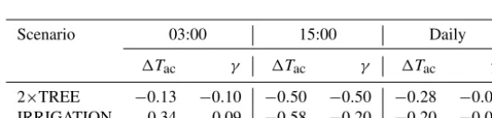
To demonstrate how TARGET can be used by practitioners to predict GBI cooling impacts, two simple heat mitigation scenarios are presented: (1) a doubling of existing tree cover (“2×TREE”) (Fig. 9) and (2) all dry grass converted to irri-gated grass (“IRRIGATION”) (Fig. 10). The 2×TREE sce-nario assumes a maximum tree coverage of 75 %. The results presented here represent the local maximum cooling poten-tial of GBI. In reality, the cooling local magnitude will be decreased by advection, which TARGET does not represent. The 2×TREE scenario shows maximum cooling of 3.0◦C during the day and a smaller effect (<0.25◦C) at night (Fig. 9). The IRRIGATION scenarios suggests that increas-ing irrigation can have a small warmincreas-ing effect (<0.75◦C) at night and cooling of up to 1.75◦C at 15:00 (Fig. 10). The amount of land cover change differs in each scenario. As such, we calculate the cooling sensitivity(γ )as
γ=
1T
ac
1LC
×0.10, (19)
where1LC is the average land cover change (fraction) (Ta-ble 2); this metric demonstrates the average1Tacper 10 %
surface change. Model results suggest that trees are about 2.5 times more effective at providing cooling at 15:00 (Ta-ble 2). The results for both heat mitigation simulations are within the expected magnitudes based on previous heat mit-igation modelling studies (Grossman-Clarke et al., 2010; Middel et al., 2015; Daniel et al., 2016; Broadbent et al., 2018a). These simulations demonstrate that TARGET not only reproduces observations accurately but can be used with confidence to efficiently assess the efficacy of heat mitigation measures.
6 Limitations of the model
As discussed above, TARGET aims to be a simple and acces-sible urban climate model that provides scientifically defen-sible and accurate urban temperature predictions. To achieve simplicity, the model necessarily makes some assumptions and omissions that users should be aware of. TARGET is primarily intended to model urban temperatures during clear sky conditions. The model does not simulate rainfall and therefore should not be used for periods containing signifi-cant precipitation. Further, the model can be used to simulate street-level air temperature and surface temperature for days to weeks (i.e. a heatwave) but has not been tested or validated for longer-scale simulations (i.e. months to years).
cool-Figure 8.Box plot of modelledTac(grey) vs. observedTac(black) for Mawson Lakes, with average, min, and maxTacshown. Box plots are generated from 30 min data from the period 15–16 February 2011. The numbers and colours (xaxis) correspond to individual stations and clusters in Fig. 3.
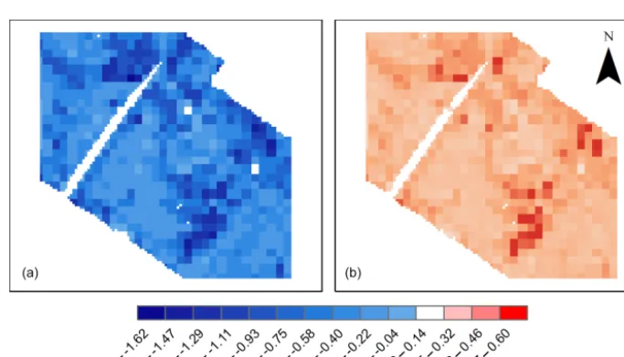
Figure 9.The1Tac(◦C) for IRRIGATION−BASE at(a)15:00 and(b)03:00 for the Mawson Lakes domain.
ing effects will be diminished by advection, especially during the day and during high wind conditions.
As mentioned, the force–restore method is used for roof and wall surfaces with an artificially reduced κ value. Al-though this approach generally performed well, it is our in-tention to develop and integrate a more realistic formula for modelling roof and wallQG,i. A conduction model, although more computationally expensive, would allow more flexibil-ity as different types of roof (which do vary significantly) could be represented. Furthermore, wall surfaces are treated the same as roofs in TARGET, which is unrealistic. The im-proved representation of walls and roofs is a key area for future model development.
In addition, theQG,i(hence the heat transfer to the urban canopy atmosphere, as the residual) is parameterized
accord-ing toRnand the building parameters. This means that the
dependency on the other atmospheric conditions, such as air temperature, wind speed, and humidity, is neglected in TAR-GET. However, given that the OHM (used to calculateQG,i) was developed based on observational data collected during summertime clear sky conditions, we are confident that TAR-GET will provide reasonable results during summer. Ongo-ing testOngo-ing is needed to ascertain the limitations of the use of the OHM in TARGET.
Figure 10.The1Tac(◦C) for 2×TREE−BASE at(a)15:00 and(b)03:00 for the Mawson Lakes domain.
Table 2.Summary of domain average cooling impacts (◦C) for GBI heat mitigation scenarios.
Scenario 03:00 15:00 Daily
1Tac γ 1Tac γ 1Tac γ
2×TREE −0.13 −0.10 −0.50 −0.50 −0.28 −0.09 IRRIGATION 0.34 0.09 −0.58 −0.20 −0.20 −0.04
for water may lead to artificial non-physical discrepancies. However, testing does not reveal any unexpected behaviour. As TARGET is a climate-service-oriented tool, we think that good model performance is more important than the consis-tency of physics schemes used.
7 Conclusions and future work
This paper has presented TARGET, a simple and user-friendly urban climate model that is designed to be accessi-ble to urban planners and policymakers. The model contains a number of key limitations that are outlined above. How-ever, despite these caveats, rigorous testing suggests TAR-GET shows excellent potential for modelling the cooling ef-fects of GBI projects. We believe this novel model is well balanced between complexity and accuracy. The computa-tional efficiency of the model and the reduced amount of in-put data required ensure that non-skilled users can use the model to ascertain reliable urban cooling estimates. Ongo-ing work will be done to improve TARGET, includOngo-ing the creation of a GUI, the addition of human thermal comfort indices, and the improvements to model physics outlined above.
Appendix A: List of symbols
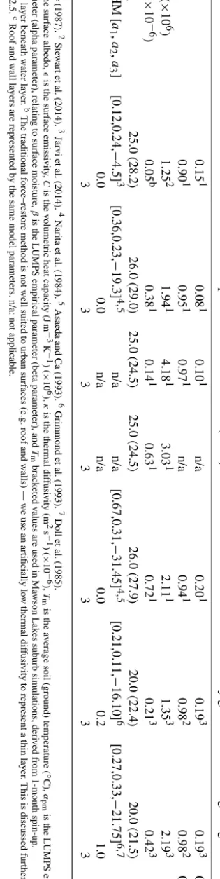
a1 Objective hysteresis model (OHM) parameter a2 Objective hysteresis model (OHM) parameter a3 Objective hysteresis model (OHM) parameter Aasph land cover asphalt plan area (m2)
Aconc land cover concrete plan area (m2) Agras land cover grass plan area (m2)
Aigrs land cover irrigated grass plan area (m2) Atree land cover tree plan area (m2)
Aroof land cover building plan area (m2) Awall land cover wall plan area (m2) Awatr land cover water plan area (m2)
Cwatr volumetric heat capacity of water (J m−2K−1)
ca conductance from the urban canopy to the above-canopy surface layer (m s−1) cs conductance from the surface to the urban canopy layer (m s−1)
Cwatr volumetric heat capacity of water (4.18×10⁶J m−3K−1) Cp specific heat of air (1013 J kg−1K−1)
dwatr depth of water body (m)
Dy damping depth for the annual temperature cycle (m)
η extinction coefficient
Fi fraction of land cover typei(%)
H average building height (m)
hc bulk transfer coefficient for heat (hc=hv)
hv bulk transfer coefficient for moisture (=1.4×10⁻³) Kn net shortwave radiation (W m−2)
K↓ incoming shortwave radiation (W m−2)
Ln net longwave radiation (W m−2) L↓ incoming longwave radiation (W m−2)
L↑ outgoing longwave radiation (W m−2)
Lv latent heat of vaporization (=2.43 MJ kg−1) QE,watr latent heat flux for water surface (W m−2)
QG,i storage heat flux for surface typeifrom LUMPS (W m−2)
QG,watr convective heat flux at the bottom of the water layer (and into the soil below) (W m−2) QH,i sensible heat flux for surfaceifrom LUMPS (W m−2)
QH,watr sensible heat flux for water surface (W m−2)
ra resistance from the urban canopy to the atmosphere (s m−1) RH relative humidity (%)
Ri Richardson number
Rn net radiation (W m−2)
Sab absorbed shortwave radiation (W m−2)
SVF sky view factor
rs resistance from the surface to the canopy (s m−1) Ta reference air temperature (◦C)
TARGET CRC for Water Sensitive Cities microclimate Toolkit model
Tac street-level (urban canopy layer) air temperature (◦C) Tb air temperature above the urban canopy layer (◦C) Tm average soil (ground) temperature (◦C)
Thigh upper-level temperature for Richardson number calculation (◦C) Tlow lower-level temperature for Richardson number calculation (◦C) Tsoil soil temperature (◦C)
Ucan wind speed in canyon (m s−1)
Utop wind speed at the top of the canyon (m s−1) Uz reference wind speed (m s−1)
W average street width (m)
W∗ average street width minus tree width (m)
Wtree tree width (m) Wroof roof width (m)
α surface albedo
αpm LUMPS empirical parameter (alpha parameter), relating to surface moisture β LUMPS empirical parameter (beta parameter)
βk amount of shortwave radiation immediately absorbed by the water layer (set to 0.45)
1QS,watr change in heat storage of the water layer (W m−2) surface emissivity
κ thermal diffusivity (m2s−1)
κwatr eddy diffusivity of water (m2s−1) λC plan area ground-level surfaces (m2)
ρa density of dry air (i.e. 1.2 kg m−3) ρv density of moist air (kg m−3)
σ Stefan–Boltzmann constant (5.67×10⁻⁸W m−2K−4)
Appendix B
B1 Meteorological conditions during validation periods As outlined in Sect. 3, we conduct model validation exper-iments during two different periods. A summary of the me-teorological conditions for land cover (Melbourne; Fig. B1) and suburb-scale (Mawson Lakes; Fig. B2) simulations are provided in the figures below.
B2 Tree surface temperature
To assess Ttree we obtain observational data from a tree
experiment completed in Melbourne, which included Tsurf
observations of the tree canopy (collected during February 2014). We also obtain Bureau of Meteorology meteorologi-cal forcing data for the 2014 case study period. This period (not shown) was very similar to the February 2012 period (Fig. B1) used above. The tree data confirm thatTais an
Figure B1.Meteorological conditions during the land cover validation period. Data source: Melbourne Airport Bureau of Meteorology (ID 086282) weather station.
Figure B2.Meteorological condition during the Mawson Lakes field campaign. Data source: Bureau of Meteorology Parafield Airport (ID: 023013) and Kent Town (ID: 94675) weather stations, Adelaide.
Author contributions. AMB, AMC, KAN, MD, HW, ESK, and NJT assisted with model development and design. AMB conducted model evaluation and analysis. All authors contributed to the writ-ing of the manuscript.
Competing interests. The authors declare that they have no conflict of interest.
Acknowledgements. At Monash University, Ashley M. Broadbent and Kerry A. Nice were funded by the Cooperative Research Centre for Water Sensitive Cities, an initiative of the Australian Govern-ment. While at Arizona State University, Ashley M. Broadbent was supported by NSF Sustainability Research Network (SRN) Cooperative Agreement 1444758, NSF grant EAR-1204774, and NSF SES-1520803. Matthias Demuzere and Hendrik Wouters were funded by the Cooperative Research Centre for Water Sensitive Cities. The contribution of Matthias Demuzere was funded by the Flemish regional government through a contract as a FWO (Fund for Scientific Research) post-doctoral research fellow. E. Scott Krayenhoff was supported by NSF Sustainability Research Network (SRN) Cooperative Agreement 1444758 and NSF SES-1520803.
Edited by: Astrid Kerkweg
Reviewed by: three anonymous referees
References
Acero, J. A. and Herranz-Pascual, K.: A comparison of thermal comfort conditions in four urban spaces by means of measure-ments and modelling techniques, Build. Environ., 93, 245–257, https://doi.org/10.1016/j.buildenv.2015.06.028, 2015.
Ali-Toudert, F. and Mayer, H.: Numerical study on the effects of aspect ratio and orientation of an urban street canyon on outdoor thermal comfort in hot and dry climate, Build. Environ., 41, 94– 108, https://doi.org/10.1016/j.buildenv.2005.01.013, 2006. Arya, P. S.: Introduction to Micrometeorology, Academic Press, San
Diego, USA, 2001.
Asaeda, T. and Ca, V. T.: The subsurface transport of heat and moisture and its effect on the environment: A numerical model, Bound.-Lay. Meteorol., 65, 159–179, https://doi.org/10.1007/BF00708822, 1993.
Bailey, B. N., Overby, M., Willemsen, P., Pardyjak, E. R., Mahaffee, W. F., and Stoll, R.: A scalable plant-resolving
radiative transfer model based on optimized GPU
ray tracing, Agr. Forest Meteorol., 198-199, 192–208, https://doi.org/10.1016/j.agrformet.2014.08.012, 2014.
Bailey, B. N., Stoll, R., Pardyjak, E. R., and Miller, N. E.: A new three-dimensional energy balance model for complex plant canopy geometries: Model development and improved vali-dation strategies, Agr. Forest Meteorol., 218–219, 146–160, https://doi.org/10.1016/j.agrformet.2015.11.021, 2016.
Bhumralkar, C. M.: Numerical experiments on the computation of ground surface temperature in an atmospheric general circulation model, J. Appl. Meteorol., 14, 1246–1258, 1975.
Broadbent, A. M., Coutts, A. M., Tapper, N. J., and Demuzere, M.: The cooling effect of irrigation on urban microclimate during heatwave conditions, Urban Climate, 23, 309–329, 2018a. Broadbent, A. M., Coutts, A. M., Tapper, N. J., Demuzere, M., and
Beringer, J.: The microscale cooling effects of water sensitive urban design and irrigation in a suburban environment, Theor. Appl. Climatol., 134, 1–23, 2018b.
Broadbent, A. M., Coutts, A. M., Nice, K. A., Demuzere, M., Krayenhoff, E. S., Tapper, N. J., and Woulters, H.: TARGETv1.0 Java code, Zenodo, https://doi.org/10.5281/zenodo.1310138, 2018c.
Bruse, M.: The influences of local environmental design on microclimate- development of a prognostic numerical Model ENVI-met for the simulation of Wind, temperature and humid-ity distribution in urban structures, PhD thesis, Univershumid-ity of Bochum, Bochum, Germany, 1999 (in German).
CD-adapco: http://www.cd-adapco.com/ (last access: 12 February 2019), 2011.
Ching, J., Mills, G., Bechtel, B., See, L., Feddema, J., Wang, X., Ren, C., Brousse, O., Martilli, A., Neophytou, M., Mouzourides, P., Stewart, I., Hanna, A., Ng, E., Foley, M., Alexander, P., Aliaga, D., Niyogi, D., Shreevastava, A., Bhalachandran, P., Masson, V., Hidalgo, J., Fung, J., Andrade, M., Baklanov, A., Dai, W., Milcinski, G., Demuzere, M., Brunsell, N., Pesaresi, M., Miao, S., Mu, Q., Chen, F., and Theeuwes, N.: WUDAPT: An Urban Weather, Climate, and Environmental Modeling In-frastructure for the Anthropocene, B. Am. Meteorol. Soc., 99, 1907–1924, https://doi.org/10.1175/BAMS-D-16-0236.1, 2018. Commonwealth of Australia: National Landcare Programme.
20 Million Trees Program, http://www.nrm.gov.au/national/ 20-million-trees (last access: 12 February 2018), 2017. Coutts, A. M., Harris, R. J., Phan, T., Livesley, S. J., Williams, N. S.,
and Tapper, N. J.: Thermal infrared remote sensing of urban heat: Hotspots, vegetation, and an assessment of techniques for use in urban planning, Remote Sens. Environ., 186, 637–651, 2016. Daniel, M., Lemonsu, A., and Viguié, V.: Role of watering practices
in large-scale urban planning strategies to face the heat-wave risk in future climate, Urban Climate, 23, 287–308, 2018.
Deardorff, J. W.: Efficient Prediction of Ground Sur-face Temperature and Moisture, With Inclusion of a Layer of Vegetation, J. Geophys. Res., 83, 1889–1903, https://doi.org/10.1029/JC083iC04p01889, 1978.
Demuzere, M., Harshan, S., Järvi, L., Roth, M., Grimmond, C., Masson, V., Oleson, K., Velasco, E., and Wouters, H.: Impact of urban canopy models and external parameters on the modelled urban energy balance in a tropical city, Q. J. Roy. Meteor. Soc., 143, 1581–1596, 2017.
Doll, D., Ching, J. K. S., and Kaneshiro, J.: Parameter-ization of subsurface heating for soil and concrete us-ing net radiation data, Bound.-Lay. Meteorol., 32, 351–372, https://doi.org/10.1007/BF00122000, 1985.
Elasson, I.: The use of climate knowledge in urban planning, Land-scape Urban Plan., 48, 31–44, 2000.
Erell, E. and Williamson, T.: Simulating air temperature in an urban street canyon in all weather conditions using measured data at a reference meteorological station, Int. J. Climatol., 26, 1671– 1694, https://doi.org/10.1002/joc.1328, 2006.
J. Appl. Meteorol., 38, 922–940, https://doi.org/10.1175/1520-0450(1999)038<0922:HSIUAL>2.0.CO;2, 1999.
Grimmond, C. S. B., Oke, T. R., and Cleugh, H.: The role of “rural” in comparisons of observed suburban-rural flux differ-ences, in: Exchange Processes at the Land Surface for a Range of Space and Time Scales. Proc. Yokohama Symposium, Yoko-hama, Japan, 13–16 July 1993, vol. IAHS Publi, 165–174, 1993. Grimmond, C. S. B. and Oke, T.: Turbulent Heat Fluxes in Ur-ban Areas: Observations and a Local-Scale UrUr-ban Meteorolog-ical Parameterization Scheme (LUMPS), J. Appl. Meteorol., 41, 792–810, 2002.
Grossman-Clarke, S., Zehnder, J. A., Loridan, T., and Grimmond, C. S. B.: Contribution of land use changes to near-surface air temperatures during recent summer extreme heat events in the Phoenix metropolitan area, J. Appl. Meteorol. Clim., 49, 1649– 1664, 2010.
Hicks, B. B.: Some evaluations of drag and bulk transfer coefficients over water bodies of different sizes, Bound.-Lay. Meteorol., 3, 201–213, https://doi.org/10.1007/BF02033919, 1972.
Jacobs, A. F. G., Heusinkveld, B. G., and Lucassen, D. C.: Tem-perature variation in a class A evaporation pan, J. Hydrol., 206, 75–83, https://doi.org/10.1016/S0022-1694(98)00087-0, 1998. Jacobs, A. F. G., Heusinkveld, B. G., and Berkowicz, S. M.:
Force-restore technique for ground surface temperature and moisture content in a dry desert system, Water Resour. Res., 36, 1261– 1268, 2000.
Järvi, L., Grimmond, C., and Christen, A.: The Surface Ur-ban Energy and Water Balance Scheme (SUEWS): Evalua-tion in Los Angeles and Vancouver, J. Hydrol., 411, 219–237, https://doi.org/10.1016/j.jhydrol.2011.10.001, 2011.
Järvi, L., Grimmond, C. S. B., Taka, M., Nordbo, A., Setälä, H., and Strachan, I. B.: Development of the Surface Urban Energy and Water Balance Scheme (SUEWS) for cold climate cities, Geosci. Model Dev., 7, 1691–1711, https://doi.org/10.5194/gmd-7-1691-2014, 2014.
Jones, I., George, G., and Reynolds, C.: Quantifying effects of phy-toplankton on the heat budgets of two large limnetic enclosures, Freshwater Biol., 50, 1239–1247, https://doi.org/10.1111/j.1365-2427.2005.01397.x, 2005.
Krayenhoff, E. S. and Voogt, J. A.: A microscale three-dimensional urban energy balance model for studying sur-face temperatures, Bound.-Lay. Meteorol., 123, 433–461, https://doi.org/10.1007/s10546-006-9153-6, 2007.
Krüger, E., Minella, F., and Rasia, F.: Impact of urban geome-try on outdoor thermal comfort and air quality from field mea-surements in Curitiba, Brazil, Build. Environ., 46, 621–634, https://doi.org/10.1016/j.buildenv.2010.09.006, 2011.
Kunz, R., Khatib, I., and Moussiopoulos, N.: Coupling of mesoscale and microscale models – an approach to simulate scale interac-tion, Environ. Modell. Softw., 15, 597–602, 2000.
Kusaka, H., Kondo, H., Kikegawa, Y., and Kimura, F.: A simple single-layer urban canopy model for atmospheric models: Com-parison with multi-layer and slab models, Bound.-Lay. Meteo-rol., 101, 329–358, 2001.
Lemonsu, A., Masson, V., Shashua-Bar, L., Erell, E., and Pearl-mutter, D.: Inclusion of vegetation in the Town Energy Balance model for modelling urban green areas, Geosci. Model Dev., 5, 1377–1393, https://doi.org/10.5194/gmd-5-1377-2012, 2012.
Lindberg, F., Holmer, B., and Thorsson, S.: SOLWEIG 1.0 – mod-elling spatial variations of 3D radiant fluxes and mean radiant temperature in complex urban settings, Int. J. Biometeorol., 52, 697–713, https://doi.org/10.1007/s00484-008-0162-7, 2008. Mascart, P., Noilhan, J., and Giordani, H.: A modified
pa-rameterization of flux-profile relationships in the surface layer using different roughness length values for heat and momentum, Bound.-Lay. Meteorol., 72, 331–344, https://doi.org/10.1007/BF00708998, 1995.
Masson, V.: A physically-based scheme for the urban energy bud-get in atmospheric models, Bound.-Lay. Meteorol., 94, 357–397, 2000.
Matzarakis, A., Rutz, F., and Mayer, H.: Modelling radia-tion fluxes in simple and complex environments–applicaradia-tion of the RayMan model, Int. J. Biometeorol., 51, 323–34, https://doi.org/10.1007/s00484-006-0061-8, 2007.
Matzarakis, A., Rutz, F., and Mayer, H.: Modelling radia-tion fluxes in simple and complex environments: basics of the RayMan model, Int. J. Biometeorol., 54, 131–139, https://doi.org/10.1007/s00484-009-0261-0, 2010.
Middel, A., Chhetri, N., and Quay, R.: Urban forestry and cool roofs: Assessment of heat mitigation strategies in Phoenix res-idential neighborhoods, Urban For. Urban Gree., 14, 178–186, 2015.
Mills, G., Ching, J., See, L., Bechtel, B., and Foley, M.: An In-troduction to the WUDAPT project, in: Proceedings of the 9th International Conference on Urban Climate, Toulouse, France, 20–24 July 2015.
Molina Martínez, J. M., Martínez Alvarez, V., González-Real, M. M., and Baille, A.: A simulation model for predicting hourly pan evaporation from meteorological data, J. Hydrol., 318, 250– 261, https://doi.org/10.1016/j.jhydrol.2005.06.016, 2006. Narita, K., Sekine, T., and Tokuoka., T.: Thermal properties of
ur-ban surface materials: study on heat balance at asphalt pavement, Geogr. Rev. Japan, 57, 639–651, 1984.
Nice, K. A., Coutts, A. M., and Tapper, N. J.: Development of the VTUF-3D v1. 0 urban micro-climate model to support assess-ment of urban vegetation influences on human thermal comfort, Urban Climate, 24, 1052–1076, 2018.
Oke, T.: Boundary Layer Climates, 2nd edn., Routledge, London, UK and New York, USA, 1987.
Oke, T. R. (2007). Siting and exposure of meteorological instru-ments at urban sites, in: Air pollution modeling and its ap-plication XVII, edited by: Borrego, C. and Norman, A. L., Springer, Boston, MA, 615–631, https://doi.org/10.1007/978-0-387-68854-1_66, 2007.
Oleson, K., Bonan, G., Feddema, J., Jackson, T., Vertenstein, M., and Kluzek, E.: Technical description of an urban parameteri-zation for the Community Land Model (CLMU), available at: http://opensky.ucar.edu/islandora/object/technotes:492 (last ac-cess: 12 February 2019), 2010.
OpenFOAM: http://www.openfoam.com/ (last access: 12 February 2019), 2011.
Redon, E. C., Lemonsu, A., Masson, V., Morille, B., and Musy, M.: Implementation of street trees within the solar radiative exchange parameterization of TEB in SURFEX v8.0, Geosci. Model Dev., 10, 385–411, https://doi.org/10.5194/gmd-10-385-2017, 2017. Salas De León, D. A., Alcocer, J., Ardiles Gloria, V., and
a warm monomictic tropical lake, J. Limnol., 75, 161–168, https://doi.org/10.4081/jlimnol.2016.1431, 2016.
Schlünzen, K. H., Grawe, D., Bohnenstengel, S. I., Schlüter, I., and Koppmann, R.: Joint modelling of obstacle in-duced and mesoscale changes – Current limits and challenges, J. Wind Eng. Ind. Aerod., 99, 217–225, https://doi.org/10.1016/j.jweia.2011.01.009, 2011.
Singapore Ministry of Environment and Water Resources: The Sin-gapore Green Plan 2012: Beyond Clean and Green Towards Environmental Sustainabiliity, available at: http://unpan1.un.org/ intradoc/groups/public/documents/apcity/unpan026598.pdf (last access: 12 February 2019), 2006.
Skamarock, W., Klemp, J., Dudhi, J., Gill, D., Barker, D., Duda, M., Huang, X.-Y., Wang, W., and Powers, J.: A Descrip-tion of the Advanced Research WRF Version 3, Tech. rep., https://doi.org/10.5065/D6DZ069T, 2008.
Spangenberg, J., Shinzato, P., Johansson, E., and Duarte, D.: Simu-lation of the influence of vegetation on microclimate and thermal comfort in the city of São Paulo, Revista da Sociedade Brasileira de Arborização Urbana, 3, 1–19, 2008.
Sparrow, E. and Cess, R.: Radiation heat transfer, augmented edn., Harper Collins, London, UK, 1978.
Stewart, I. D., Oke, T. R., and Krayenhoff, E. S.: Evaluation of the “local climate zone” scheme using temperature observations and model simulations, Int. J. Climatol., 34, 1062–1080, 2014. Subin, Z. M., Riley, W. J., and Mironov, D.: An improved lake
model for climate simulations: Model structure, evaluation, and sensitivity analyses in CESM1, J. Adv. Mode. Earth Syst., 4, 1– 27, https://doi.org/10.1029/2011MS000072, 2012.
Ward, H. C., Kotthaus, S., Järvi, L., and Grimmond, C. S. B.: Sur-face urban energy and water balance scheme (SUEWS): develop-ment and evaluation at two UK sites, Urban Climate, 18, 1–32, 2016.
Wouters, H., Demuzere, M., Blahak, U., Fortuniak, K., Maiheu, B., Camps, J., Tielemans, D., and van Lipzig, N. P. M.: The ef-ficient urban canopy dependency parametrization (SURY) v1.0 for atmospheric modelling: description and application with the COSMO-CLM model for a Belgian summer, Geosci. Model Dev., 9, 3027–3054, https://doi.org/10.5194/gmd-9-3027-2016, 2016.