Determining the Relative Importance of Parameters Affecting Concrete Pavement Thickness

journal homepage: http://civiljournal.semnan.ac.ir/

Determining the Relative Importance of Parameters

Affecting Concrete Pavement Thickness

Gh. Shafabakhsh1*, H. Naderpour2 and R. Noroozi3

1. Associate Professor, Department of Civil Engineering, Semnan University, Semnan, Iran. 2. Assistant Professor, Department of Civil Engineering, Semnan University, Semnan, Iran. 3. Ph.D. student, Department of Civil Engineering, Semnan University, Semnan, Iran.

Corresponding author:[email protected]

ARTICLE INFO ABSTRACT

Article history:

Received: 27 August 2014 Accepted: 07 May 2015

To manage costs and optimize the thickness of concrete pavements, recognizing the amount of determinative factors’ influence will be required. A study with the aim of determining the influence of traffic parameters, type of subgrade soil and the base layer thickness on the concrete pavement slab thickness can provide the choice of best concrete pavement design. For this purpose, the PCASE software has been used in this paper to produce sufficient number of numerical examples, 288 samples, with taking into account the number of equivalent single axle, the subgrade modulus and the base layer thickness. These samples are considered as the basis of training and testing an artificial neural network and the level of pavement design parameters importance is relatively determined on the results of optimal neural network. The method used in this paper for calculating the relative importance of each parameter involved in the concrete pavement thickness indicates that the parameters of base layer thickness and the number of equivalent single axle have the lowest and highest level of influence, with the values of about 21 and 42 percent, respectively. The obtained results are also compatible with concepts and structural features of concrete pavements.

Keywords:

Concrete pavement, Pavement design, PCASE,

Neural network, Relative importance.

1. Introduction

The existence of substantial advantages and benefits of applying concrete pavement in roads is turned this type of pavement into one of the most likely options of designer

Although the existence of various methods and software provides the possibility of preparing appropriate designs, the amount of influence of each parameters involved in the design of concrete pavements is still ambiguous. Among the most well-known methods proposed for concrete pavement design, the AASHTO Guide for the design of pavement structures which has been published in 1986 can be noted [1,2]. Also, Kentucky Rigid Pavement Design, Portland Cement Association (PCA) and American Concrete Pavement Association which have less input parameters as compared with the AASHTO method, can be cited [3]. Different design software are of appropriate tools as an alternative to the above methods. The software used in this study is Pavement-Transportation Computer Assisted Structural Engineering which is briefly called PCASE [4]. This software has been developed by the U.S. Army Corps of Engineers association and its 2008 version is available to the public as the latest version [5]. In this paper, the results obtained from the software have been employed for training and testing an artificial neural network and then the contribution of the influence of parameters involved in the design of concrete pavement has been analyzed.

Sensitivity analysis is discussed as a prerequisite for the time consuming and costly processes of validation the numerical and field data, because by means of it, the important variables of the model and rational assumptions for variables are determined without disturbing in process of predictions [6]. Sensitivity analysis on issues related to the concrete pavements have been used by various researchers [7–9]. In these cases, variables effect is mainly considered

separately, it means that in these studies, one variable has been changed at a time and the other parameters have been assumed fixed. In this research, in order to simultaneously and comprehensively investigate the variables affecting the thickness of concrete pavement slab, artificial neural networks have been applied as a powerful tool to determine the design relationships and a popular method to estimate the importance of each of the variable parameters in these networks.

compared with respect to the input neurons [18]. Also, in the input perturbation method, changes in the Mean Square Error (MSE) of the network are assessed for small changes in each input neuron [19]. The changes results in the Mean Square Error for each input perturbation explain the relative importance of predicted variables [20].

Garson’s Algorithm is also considered as another method used in this subject that partitions hidden-output connection weights into components associated with each input neuron using the absolute values of connection weights [21]. In this study, the method proposed by Garson which is called "Weights" in some researches, has been utilized [19].

This paper presents estimating the contribution of concrete pavement design parameters affecting pavement slab thickness. The contribution of input parameters in predicted output, has been specified by using the weight gained in the optimal Feed-Forward back propagation neural network for each of the input parameters, including the number of equivalent axle, pavement subgrade modulus, the amount of base layer thickness and the output parameter of the pavement layer thickness. Feed-Forward back propagation neural networks are considered as the most widely used systems of neural networks [22]. As a result of this research, the type of road pavement can be determined for optimal conditions. Because the amount of desired thickness can be selected for places with optimal traffic conditions, the optimal conditions of subgrade soil and the most optimal conditions of base layer thickness.

2. Materials and Methods

2.1. Data Characteristics

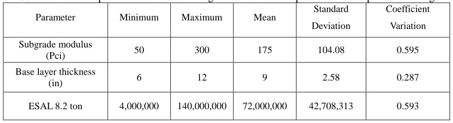
Since the characteristics of subgrade soil and the rate of passing traffic are discussed as the mandatory characteristics in determining the pavements thickness, they have been applied in the process of relative importance determination. Also, applying an embankment layer with relatively high quality material is applicable as a known method to reduce the pavement thickness. Thus, in the following, components of the number of passing equivalent axle in the year of design, the subgrade soil reaction modulus and the base layer thickness in accordance with ranges mentioned in Table 1 have been studied and evaluated. Parameters range are selected to coverage the variety condition. It means by this range of data, weak to strong subgrade, customary thickness of base layers and every possible traffic volume are considered.

From the combination of the items listed in Table 1, 288 samples of concrete pavement design are obtained that these numbers are modeled in PCASE software and the required concrete pavement thickness appropriate for them are calculated.

2.2. PCASE Software

Table 1. The assumptions used in determining the numerical samples of concrete pavement design

Parameter Minimum Maximum Mean Standard

Deviation

Coefficient

Variation

Subgrade modulus

(Pci) 50 300 175 104.08 0.595

Base layer thickness

(in) 6 12 9 2.58 0.287

ESAL 8.2 ton 4,000,000 140,000,000 72,000,000 42,708,313 0.593

This software has the ability to design and assess flexible and rigid road and airport pavements based on CBR, k method and the LED analytical method. The software has collected all evaluation and design criteria of road and airport in a collection [5].

The samples mentioned in the previous paragraph have been modeled by the software and the corresponding pavement thickness obtained has been used for training and testing the optimal artificial neural network.

2.3. Artificial Neural Network (ANN)

NNs are parallel connectionist structures constructed to simulate the working network of neurons in the human brain [14]. This structure derived from the human brain performance, during a learning process and with the help of processors called neurons acquires the ability to discover intrinsic relationships between data and by this means suggests the relationship between input and output parameters. NNs operate as black-box, model-free and adaptive tools to capture and learn significant structures in data [23]. The first idea of applying ANNs can be attributed to McCulloch and Pitts in 1943 [24]. The scientists were inspired from the self-learning and automatic operation of brain and nerve systems. The ANN computing abilities have been proven in the field of tackling complex

pattern-recognition problems widely [25–29]. The broad advantages of this system have led many researchers to advocate ANN systems as an attractive, non-linear alternative to traditional statistical methods [17].

In this study, an artificial neural network prediction model has been used to examine how PCASE Software responds to independent input values and determining the concrete pavement thickness. To do this, the multi-layer Feed-Forward network, that is the most popular of network architectures currently available in the field of engineering, has been utilized [19,30]. The multi-layer Feed-Forward networks consist of an input layer, one or more hidden layers and an output layer that each layer is composed of a number of neurons or nodes. The number of neurons in the input and output layers system is defined by the number of variables in the system, while neurons in the hidden layer(s) is usually determined by using a trial and error process. The overall structure of the three-layer Feed-Forward network is shown in Fig. 1. As seen in the figure, the neurons of each layer are connected to neurons of the next layer by weights.

signals, xi for i = 0, 1, 2, ..., n and then applies a nonlinear function to produce an output signal, uj. A simple model of a neuron is shown in Fig. 1. A neuron j is described mathematically by the following pair of equations:

𝑢𝑗 = ∑𝑝𝑖=1𝑤𝑖𝑗. 𝑥𝑖 (1)

𝑥_𝑗 = φ(𝑢_𝑗− 𝜃_𝑗) (2)

Where θ is a threshold function and its use has the effect to apply an affine transformation to the output of the linear combiner in the model of Fig. 1 [31,32]. In this study, the logistic sigmoid nonlinear function [33] is used for this purpose, expressed as:

𝜑_𝑥 =_1+𝑒1_−𝑥 (3)

Fig. 1. Architecture of a neural network and input and output parameters [28]

Fig. 2. The nonlinear model of a neuron [31] The training and testing process of neural network used in this study have been conducted by applying 288 concrete pavement design models prepared by PCAE Software. Due to the utilization of sigmoid function as transfer function in the network construction steps, before the optimization of neural network, all dependent and independent variables have been standardized in order to achieve a specified distribution. In fact, all the variables of 288 numerical samples have been prepared for entering the neural network environment. Neural Network toolbax of Matlab software is utilized here to determination the correlation between networks layer's neurons and associated weights based on Eq. (1-3).

In the back propagation algorithm employed in this study, monitoring the generated error value is used to examine how convergence arises. This process is calculated by the square root equations and can be obtained as the Mean Squared Error (MSE) as follows [31]:

𝑀𝑆𝐸 = _𝑀𝑃1 ∑ ∑𝑀 (𝑑_𝑘− 𝑦_𝑘)2 𝑘=1

𝑃

1 (4)

2.4. Index of Relative Importance

In the sensitivity analysis processes, the rate and the way of input data distribution with the highest impact on the model output is determined. With this process, the trial and error steps in the design process can be reduced and the most important effective parameters can be identified. Based on the methodology, sensitivity analysis methods can be classified as mathematical, statistical and graphical techniques. This classification can be done based on the capabilities and applicability of a specific method as well. Generally, applicable methods for assessing the contribution of independent variables in neural networks have some complexities. For example, intensive computational approaches such as growing and pruning algorithms [34], partial derivatives [18,35] and asymptonic t-tests are often not used in favour of simpler techniques that use the network connection weights (e.g. Garson’s algorithm [21]; Lek’s algorithm [36]; saliency analysis [37]; [38]).

Generally, as shown in Fig. 3, the current methods for the analysis of the effect or importance of the input variables on the outputs of back propagation neural network can be classified into two main categories: analysis based on the magnitude of weights and sensitivity analysis. Since the late of 1980s these methods have been proposed for interpreting what has been learned by a back-propagation network composed of input neurons, hidden neurons and output neurons.

Analysis based on the magnitude of weights groups together those procedures that are based exclusively on the values stored in the static matrix of weights to determine the relative influence of each input variable on each one of the network outputs [39]. Different equations have been proposed based on the weights magnitude, all of them characterized by the calculation of the connection weights between input neurons and hidden neurons and the connection weights between hidden neurons and output neurons for each of the hidden neurons of the network, obtaining the sum of the calculated products.

The procedure for partitioning the connection weights to determine the relative importance of the various inputs was proposed first by Garson (1991) and repeated by Goh (1995). The method essentially involves partitioning the hidden-output connection weights of each hidden neuron into components associated with each input neuron [19].

In this study, in order to determine the relative importance of input variables on concrete pavement thickness, assessment process based on the weight matrix of the proposed optimized network and Garson’s modified equation have been used. The equation is as follows:

𝐼𝑗 =

∑ (( |𝑊𝑗𝑚𝑖ℎ |

∑𝑘=𝑁𝑖_{𝑘=1 |𝑊𝑘𝑚}𝑖ℎ |)×|𝑊𝑚𝑛 ℎ𝑜_|) 𝑚=𝑁ℎ

𝑚=1

Fig. 3. Introducing the methods of determining the influence of input parameters on the network output [39]

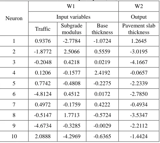
Table 2. The weight matrix, weights between input and hidden layers (W1) and the weights between the hidden and output layers (W2)

Neuron

W1 W2

Input variables Output

Traffic Subgrade modulus

Base thickness

Pavement slab thickness

1 0.9376 -2.7784 -1.0724 1.2645

2 -1.8772 2.5066 0.5559 -3.0195

3 -0.2048 0.4218 0.0219 -4.1667

4 0.1206 -0.1577 2.4192 -0.0657

5 0.7742 -0.4808 -0.2275 -2.2339

6 -4.8124 0.4512 0.0172 -2.7850

7 0.4972 -0.1759 0.4222 -0.4934

8 -0.5147 1.7713 -0.5724 -3.5347

9 -4.6734 -0.3285 -0.0029 -2.2112

10 2.0888 -4.2969 -0.6365 -1.4424

Where, Ij is the relative importance of the jth input variable on the output variable, Ni and Nh are the number of input and hidden neurons, respectively and W is connection weight, the superscripts i, h and o refer to input, hidden and output layers, respectively and subscripts k, m and n refer to input, hidden and output neurons, respectively [40]. Table 2. demonstrates the weights values produced between artificial neurons of the neural network model used in this study.

Weights presented in table come from Neural Network toolbox of Matlab software.

3. Results and Discussion

In this study, data sets obtained from the concrete pavement design have been utilized in two parts: training data and testing data. In the training phase, 288 samples of pavement design, as mentioned in section 2.1, have been employed and 124 samples in the determining the

influence of input parameters

Analysis based on the weights

magnitude

Analysis based on error function

Analysis based on network output

Numeric method

testing phase, approximately 50 percent of whole data, have been used. A Feed-Forward back propagation network has been considered to predict the concrete pavement thickness needed. Neurons in the input layer lack transfer function and for the hidden layer, the sigmoid transfer function has been used. Network has been trained using Levenberg-Marquardt algorithm.

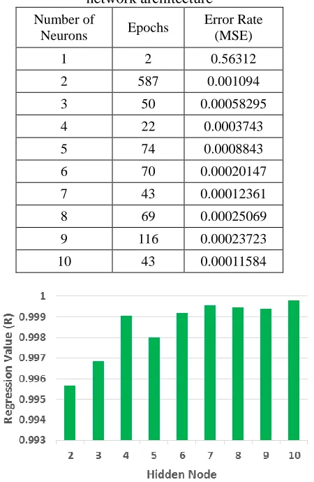
In order to determine the optimum arrangement and architecture, samples of Feed-Forward networks with increasing number of neurons in the hidden layer from 1 to 10 neurons have been examined. Table 3 reports the control outputs achieved in the selection steps of the optimum arrangement of the neural network. In Fig. 4, the total correlation coefficient value for the networks examined is also displayed. As these comparisons show, the best number of neurons usable in the hidden layer of neural network, considering the mean square error and the total correlation coefficient, is 10 neurons. Because, by selecting this number of neuron in the hidden layer, firstly, the MSE has the lowest value, and secondly, the correlation coefficient (regression) has the highest value between the architectures investigated, that this means the greatest agreement between the values predicted by the network with 10 neurons in the hidden layer with the values obtained from PCASE Software. It should be noted that the number of epoch is considered as the representative of simulation time and due to the negligible importance of processing speed in modern computer systems, it has been removed from the review process. With these interpretations, the arrangement of (1, 10, 3) will be as the optimum proposed arrangement to determine the appropriate thickness of concrete pavement by the

Feed-Forward back propagation network. In the following and in Figs. 5 and 6, the results of the training and testing steps of the selected network are presented.

Table 3. details of the selection of optimal network architecture

Error Rate (MSE) Epochs

Number of Neurons

0.56312 2

1

0.001094 587

2

0.00058295 50

3

0.0003743 22

4

0.0008843 74

5

0.00020147 70

6

0.00012361 43

7

0.00025069 69

8

0.00023723 116

9

0.00011584 43

10

Fig. 4. Correlation coefficient of different networks

Fig. 5. MSE error rate obtained in the training and testing periods of the network with the arrangement of (10, 1, 3)

Fig. 7. The test results of the selected optimal neural network After determining the optimal architecture of

the back propagation neural network and examining the results of correlation coefficient of the model in Figs. 6 and 7, as presented in Table 2, the weight values corresponding to the input and output variables have been determined by Garson’s equation in order to estimate the amount of importance or influence of the model inputs on the output corresponding to them. The results obtained indicating the effectiveness of each of the input variables on the output of the network or the concrete pavement slab thickness, are shown in Fig. 8.

Fig. 8. The effect of three variables on the pavement slab thickness

4. Conclusions

According to obtained result of current study, the back propagation neural network with the arrangement of 3, 10, 1 can provide a very high correlation coefficient close to 1 that is applicable for concrete pavement design purposes. However, the study of the relationships between neural network's layer neurons with the external physical environment is relatively unknown. In the other words, comprehensive understanding of how the relationship of network weights with the response values of hidden neurons as a set of training data, is not possible. Thus, in neural networks, in contrast to classical statistical models, finding the effect of the independent variable on the dependent variable is not simply gained. For this purpose, and in order to determine the amount of influence of traffic flow parameters, subgrade soil resistance and base layer thickness, the relative importance of each of these parameters have been determined based on weights between produced artificial neurons in the network.

6 6.2 6.4 6.6 6.8 7 7.2 7.4

6 6.2 6.4 6.6 6.8 7 7.2 7.4

Pre

dic

te

d

PC

C

T

hic

kn

ess

Designed PCC Thickness

0 5 10 15 20 25 30 35 40 45

Traffic Subgrade

Modulus

Base Thickness

Rel

ati

ve

Impo

rta

n

ce

This process has been done by Garson’s modified equation (Eq. 5).

The obtained results in this study suggest that the number of single axle load of passing traffic, has the greatest effect (42.35%) on the concrete pavement slab thickness. This finding reveals the significant difference of pavement slab thickness used in the roads with different roles, from rural to arterials. The modulus of subgrade soil reaction is considered as the second determinative component of the concrete pavement slab thickness. The amount of influence of this parameter has reached to 36.65% and shows the importance of the amount of soil resistance of pavement slab construction place in a grade lower than the amount of traffic load movement. The base layer thickness is considered as the least effective component in the concrete pavement design process. The amount of influence of 21% for the base layer thickness indicates the relatively low importance and its little impact on the required pavement slab thickness. This matter introduces the base layer applying as low-impact options for saving in consuming concrete of pavement slab.

REFERENCES

[1] Fogg, J. A., Baus, R. L., Ray, R. P. (1991). “AASHTO rigid pavement design equation study”, J. Transp. Eng., vol. 117, no. 1, pp. 124–131.

[2] Guclu, A., Ceylan, H. (2005). “Sensitivity Analysis of Rigid Pavement Systems Using Mechanistic-Empirical Pavement Design Guide”, in Proceedings of the 2005 Mid-Continent Transportation Research Symposium, Ames, Iowa.

[3] Southgate, H. F. (1988). “Comparison of rigid pavement thickness design systems”, Research Report UKTRP-88-14, Lexington, Kentuchy.

[4] Jersey, S. R., Bell, H. P. (2011). “Analyses of Structural Capacity of Rigid Airfield Pavement Using Portable Seismic Technology”, Int. J. Pavement Res. Technol., vol. 4, no. 3, pp. 147–153. [5] Taghavi Esfandani, M., Mansourian, A.,

Babaei, A. (2013). “Investigation of Runway Pavement Design Software and Determination of Optimization Software”, J. Basic Appl. Sci. Res., vol. 3, no. 4, pp. 143–150.

[6] Kannekanti, V., Harvey, J. (2006). “Sensitivity analysis of 2002 design guide distress prediction models for jointed plain concrete pavement”, Transp. Res. Rec. J. Transp. Res. Board, vol. 1947, no. 1, pp. 91–100.

[7] Hall, K. D., Beam, S. (2005). “Estimating the sensitivity of design input variables for rigid pavement analysis with a mechanistic-empirical design guide”, Transp. Res. Rec. J. Transp. Res. Board, vol. 1919, no. 1, pp. 65–73.

[8] Khazanovich, L., Darter, M. I., Yu, H. T. (2004). “Mechanistic-empirical model to predict transverse joint faulting”, Transp. Res. Rec. J. Transp. Res. Board, vol. 1896, no. 1, pp. 34–45.

[9] Mallela, J., Abbas, A., Harman, T., Rao, C., Liu, R., Darter, M. I. (2005). “Measurement and significance of the coefficient of thermal expansion of concrete in rigid pavement design”, Transp. Res. Rec. J. Transp. Res. Board, vol. 1919, no. 1, pp. 38–46.

[10] Attoh-Okine, N. O., Cooger, K., Mensah, S. (2009). “Multivariate adaptive regression (MARS) and hinged hyperplanes (HHP) for doweled pavement performance modeling”, Constr. Build. Mater., vol. 23, no. 9, pp. 3020–3023.

[11] Bayrak, M. B., Ceylan, H. (2008). “Neural network-based approach for analysis of rigid pavement systems using deflection data”, Transp. Res. Rec. J. Transp. Res. Board, vol. 2068, no. 1, pp. 61–70.

load and thermal effects during reflection cracking”, J. Mater. Civ. Eng., vol. 23, no. 3, pp. 221–229.

[13] Ceylan, H., Gopalakrishnan, K. (2007). “Neural Networks Based Models for Mechanistic-Empirical Design of Rubblized Concrete Pavements”, Geotech. Spec. Publ. No. 169, Soil Mater. Inputs Mech. Pavement Des. ASCE, pp. 1–10. [14] Gopalakrishnan, K. (2010). “Effect of

training algorithms on neural networks aided pavement diagnosis”, Int. J. Eng. Sci. Technol., vol. 2, no. 2, pp. 83–92. [15] Sharma, S., Das, A. (2008).

“Backcalculation of pavement layer moduli from falling weight deflectometer data using an artificial neural network”, Can. J. Civ. Eng., vol. 35, no. 1, pp. 57–66. [16] Kisi, O. (2005). “Daily river flow forecasting using artificial neural networks and auto-regressive models”, Turkish J. Eng. Environ. Sci., vol. 29, no. 1, pp. 9–20. [17] Olden, J., Jackson, D. (2002). “Illuminating the ‘black box’: a randomization approach for understanding variable contributions in artificial neural networks”, Ecol. Modell., vol. 154, no. 1–2, pp. 135–150.

[18] Dimopoulos, Y., Bourret, P., Lek, S. (1995). “Use of some sensitivity criteria for choosing networks with good generalization ability”, Neural Process. Lett., vol. 2, no. 6, pp. 1–4.

[19] Gevrey, M., Dimopoulos, I., Lek, S. (2003). “Review and comparison of methods to study the contribution of variables in artificial neural network models”, Ecol. Modell., vol. 160, no. 3, pp. 249–264. [20] Scardi, M., Harding Jr, L. W. (1999).

“Developing an empirical model of phytoplankton primary production: a neural network case study”, Ecol. Modell., vol. 120, no. 2, pp. 213–223.

[21] Garson, G. D. (1991). “Interpreting neural-network connection weights”, AI Expert, vol. 6, no. 4, pp. 46–51.

[22] Flood, I., Kartam, N. (1994). “Neural networks in civil engineering. I: Principles and understanding”, J. Comput. Civ. Eng., vol. 8, no. 2, pp. 131–148, 1994.

[23] Adeli, H. (2001). “Neural Networks in Civil Engineering: 1989-2000”, Comput. Civ. Infrastruct. Eng., vol. 16, no. 2, pp. 126– 142, Mar. 2001.

[24] McCulloch, W. S., Pitts, W. (1943). “A logical calculus of the ideas immanent in nervous activity”, Bull. Math. Biophys., vol. 5, no. 4, pp. 115–133, 1943.

[25] Chen, D. G., Ware, D. M. (1999). “A neural network model for forecasting fish stock recruitment”, Can. J. Fish. Aquat. Sci., vol. 56, no. 12, pp. 2385–2396.

[26] Manel, S. S. , Dias, J.-M., Ormerod, S. J. (1999). “Comparing discriminant analysis, neural networks and logistic regression for predicting species distributions: a case study with a Himalayan river bird”, Ecol. Modell., vol. 120, no. 2, pp. 337–347. [27] Özesmi, S. L., Özesmi, U. (1999). “An

artificial neural network approach to spatial habitat modelling with interspecific interaction”, Ecol. Modell., vol. 116, no. 1, pp. 15–31.

[28] Paruelo, J., Tomasel, F. (1997). “Prediction of functional characteristics of ecosystems: a comparison of artificial neural networks and regression models”, Ecol. Modell., vol. 98, no. 2, pp. 173–186.

[29] Spitz, F., Lek, S. (1999). “Environmental impact prediction using neural network modelling. An example in wildlife damage”, J. Appl. Ecol., vol. 36, no. 2, pp. 317–326.

[30] Mural, R. V., Puri, A. B., Prabhakaran, G. (2010). “Artificial neural networks based predictive model for worker assignment into virtual cells”, Int. J. Eng. Sci. Technol., vol. 2, no. 1, pp. 163–174. [31] Haykin, S. (1999). “Neural networks: a

comprehensive foundation 2nd edition”,

Up. Saddle River, NJ, US Prentice Hall.

[32] Melesse, A. M., Hanley, R. S. (2005). “Artificial neural network application for multi-ecosystem carbon flux simulation”, Ecol. Modell., vol. 189, no. 3, pp. 305– 314.

station using reference stations data”,

Renew. Energy, vol. 32, no. 14, pp. 2350–

2360.

[34] Bishop, C. M. (1995). "Neural networks for pattern recognition", vol. 92, no. 440. Clarendon press Oxford, p. 498.

[35] Dimopoulos, I., Chronopoulos, J., Chronopoulou-Sereli, A., Lek, S. (1999). “Neural network models to study relationships between lead concentration in grasses and permanent urban descriptors in Athens city (Greece)”, Ecol. Modell., vol. 120, no. 2, pp. 157–165.

[36] Lek, S., Delacoste, M., Baran, P., Dimopoulos, I., Lauga, J., Aulagnier, S. (1996). “Application of neural networks to modelling nonlinear relationships in ecology”, Ecol. Modell., vol. 90, no. 1, pp. 39–52.

[37] Abrahart, R. J., See, L., Kneale, P. E. (2001). “Investigating the role of saliency analysis with a neural network rainfall-runoff model”, Comput. Geosci., vol. 27, no. 8, pp. 921–928.

[38] Makarynskyy, O., Makarynska, D., Kuhn, M., Featherstone, W. E. (2004). “Predicting sea level variations with artificial neural networks at Hillarys Boat Harbour, Western Australia”, Estuar. Coast. Shelf Sci., vol. 61, no. 2, pp. 351– 360.

[39] Montano, J., Palmer, A. (2003). “Numeric sensitivity analysis applied to feedforward neural networks”, Neural Comput. Appl., vol. 12, no. 2, pp. 119–125.