https://doi.org/10.5194/gmd-12-3541-2019 © Author(s) 2019. This work is distributed under the Creative Commons Attribution 4.0 License.
The upper-atmosphere extension of the ICON general
circulation model (version: ua-icon-1.0)
Sebastian Borchert1, Guidi Zhou2,a, Michael Baldauf1, Hauke Schmidt2, Günther Zängl1, and Daniel Reinert1 1Deutscher Wetterdienst, Offenbach am Main, Germany
2Max Planck Institute for Meteorology, Hamburg, Germany
acurrently at: College of Oceanography, Hohai University, Nanjing, China Correspondence:Sebastian Borchert ([email protected]) Received: 15 November 2018 – Discussion started: 20 December 2018 Revised: 12 July 2019 – Accepted: 15 July 2019 – Published: 14 August 2019
Abstract. How the upper-atmosphere branch of the circu-lation contributes to and interacts with the circucircu-lation of the middle and lower atmosphere is a research area with many open questions. Inertia–gravity waves, for instance, have moved in the focus of research as they are suspected to be key features in driving and shaping the circulation. Nu-merical atmospheric models are an important pillar for this research. We use the ICOsahedral Non-hydrostatic (ICON) general circulation model, which is a joint development of the Max Planck Institute for Meteorology (MPI-M) and the German Weather Service (DWD), and provides, e.g., local mass conservation, a flexible grid nesting option, and a non-hydrostatic dynamical core formulated on an icosahedral– triangular grid. We extended ICON to the upper atmosphere and present here the two main components of this new con-figuration named UA-ICON: an extension of the dynamical core from shallow- to deep-atmosphere dynamics and the im-plementation of an upper-atmosphere physics package. A se-ries of idealized test cases and climatological simulations is performed in order to evaluate the upper-atmosphere exten-sion of ICON.
1 Introduction
In climate simulations and numerical weather prediction (NWP), there are ongoing efforts to raise the upper model lid, acknowledging possible influences of middle- and upper-atmosphere dynamics on tropospheric weather and climate (e.g., Thompson et al., 2002; Scaife et al., 2012; Charlton-Perez et al., 2013). The dynamics of the large-scale flow
in the middle and upper atmosphere is determined, for in-stance, by the interaction with small-scale gravity waves. These waves, predominantly forced in the troposphere, can propagate vertically until they become unstable and break. As a result of this, a drag is exerted on the atmospheric back-ground flow. This is an important route of momentum flux from the lower atmosphere to the middle and upper atmo-sphere, which shapes the meridional circulation in the latter regions (e.g., Fritts and Alexander, 2003; Kim et al., 2003). To have a model at hand that allows to study such processes on a wide range of spatial and temporal scales was one of our central motivations for the upper-atmosphere extension of the ICON model, which we present in the following.
dis-tinct packages of physics parameterizations, ICON meets the different needs of climate simulations, NWP and LES. To prepare ICON for simulations with model tops in the lower thermosphere, some extensions of the dynamical core and the physics parameterizations are necessary, as presented in this work.
Among the most important approximations which are ap-plied to the dynamical core of ICON in its standard config-uration are the shallow-atmosphere approximation and tradi-tional approximation (e.g., Phillips, 1966; White and Brom-ley, 1995; White et al., 2005; Staniforth and Wood, 2008). These approximations are applied to the mapping of the bud-get equations on spherical coordinates relative to the center of the Earth. The shallow-atmosphere approximation is ba-sically associated with the neglect of terms related to the spherical curvature of the atmosphere as well as variations of the gravitational field by assuming the field strength to be constant (see Thuburn and White, 2013, for a detailed exam-ination of the metrical implications of this approximation). The traditional approximation refers to neglecting the contri-bution of the horizontal component of the Earth’s angular ve-locity to the Coriolis acceleration. Following the usual termi-nology, we will call the system of equations with and without the two approximations the shallow-atmosphere equations and deep-atmosphere equations, respectively. Both approx-imations are generally applied together in order to satisfy the conservation of the energy, the axial component of angular momentum, and the potential vorticity (e.g., Phillips, 1966; White and Bromley, 1995; Staniforth and Wood, 2003). However, as Tort and Dubos (2014) have shown, it is pos-sible to extend the shallow-atmosphere equations in such a way that the full Coriolis acceleration can be retained with-out violating the conservation principles.
The accuracy of the shallow-atmosphere and traditional approximations can be estimated by comparing the magni-tude of the terms neglected in the shallow-atmosphere equa-tions to the magnitude of the terms that are present in both systems. Such scale analysis has been used, for instance, by White and Bromley (1995), to show that for diabatically driven flows in the tropics and planetary-scale flows the ne-glected terms of the Coriolis acceleration might reach mag-nitudes up to about 10 % of the magnitude of key terms of the shallow-atmosphere momentum budget. On the other side, normal-mode analyses, done by Thuburn et al. (2002a) for the deep-atmosphere equations, and by Kasahara (2003) with focus on a Boussinesq model featuring the full Coriolis acceleration, show that the differences in the spatial struc-ture and the frequencies of the energetically most significant modes between the shallow- and the deep-atmosphere equa-tions are relatively small (with differences in the frequency magnitude being typically less than about 1 %; Thuburn et al., 2002b; Kasahara, 2003). Both, the scale analysis and the normal-mode analysis are important tools to figure out the differences between the deep- and shallow-atmosphere equations. However, the applicability of the results on
long-term integrations might be limited. The systematic errors in-troduced by the approximations, albeit small in magnitude, could accumulate over time and lead to significantly differ-ent flow patterns of the model atmosphere. This might be especially important for the large-scale circulations of the middle and upper atmosphere. Furthermore, in view of the ever-increasing computational power, some approximations that were meaningful under the restrictions of past computer architectures might nowadays lose their justification. There-fore, we decided to expand the dynamical core of ICON by a deep-atmosphere option.
Examples for other models that use a deep-atmosphere formulation, or offer the option to do so, are the Met Of-fice’s Unified Model (UM) (Davies et al., 2005; Wood et al., 2014), the Non-hydrostatic Icosahedral Atmospheric Model (NICAM) (e.g., Tomita and Satoh, 2004), the Ocean Land Atmosphere Model (OLAM) (e.g., Walko and Avissar, 2008), the MCore model by Ullrich and Jablonowski (2012), and the Finite Volume Model (FVM) of the Integrated Fore-casting System (IFS) developed at the European Centre for Medium-Range Weather Forecasts (ECMWF) (e.g., Smo-larkiewicz et al., 2016). An overview of some of these models can be found in Ullrich et al. (2017).
Apart from the dynamics, the physics parameterizations are the second important model pillar that has to be extended for applications including part of the upper atmosphere. The ICON model offers basically three different physics pack-ages: one which has been largely adopted from the ECHAM model intended for climate simulations (e.g., Stevens et al., 2013; Giorgetta et al., 2018; Crueger et al., 2018), another one which is used for NWP (some aspects of which can be found in Zängl et al., 2015), and a third one for LES (Di-pankar et al., 2015). The upper-atmosphere-specific physics parameterizations have been integrated into the ECHAM and NWP packages, but we will focus on the extended ECHAM physics package in the remainder of this work. To avoid con-fusion in the following, a side note on our terminology may be in order: if we discuss the physics parameterizations, we typically use the attribute “upper atmosphere” to denote that their effects become significant in and above, say, the upper-mesosphere–lower-thermosphere region. In contrast, the at-tribute “deep atmosphere” is used in the context of the modi-fications of the dynamical core, since they apply to the entire air column, and no more or less well-defined vertical signif-icance threshold can be made out for them. If we address both extensions as a whole, we use again the attribute “upper atmosphere”.
the characteristics of the upper atmosphere, most importantly the rarefied air and the broader spectrum of incoming solar irradiance, which give rise to some physical phenomena that are negligible in the lower atmosphere and thus not parame-terized in the current model but become crucial in maintain-ing the upper-atmospheric dynamics and thermodynamics.
One of such physical phenomena is molecular diffusion of momentum and heat, which is of negligible magnitude in the lower atmosphere compared to turbulent diffusion. In the upper atmosphere, as turbulence dies away and the air molecules are capable of traveling a long distance, molec-ular diffusion becomes dominant. Besides molecules, the upper atmosphere is also abundant with atoms and radi-cals produced as a result of photolysis. Chemical heating is the release of heat by recombination reactions between atoms or radicals, and is of particular importance in the up-per atmosphere where photolysis products can travel large distances before recombining. Moreover, the higher altitude also means that the upper atmosphere would receive and ab-sorb more solar irradiance in higher frequencies than at lower levels and on the surface. This brings the need of param-eterizing the ultraviolet radiation including the Schumann– Runge bands and continuum, and the extreme ultraviolet bands. The solar radiation also acts to ionize the atmosphere, establishing the ionosphere from about 60 km. The electri-cally charged ions in the ionosphere are then aligned with the magnetic field of the Earth, thus creating a drag and a heating source to the neutral mass flow. Further, the usual as-sumption of local thermodynamical equilibrium (LTE) does not hold in the upper atmosphere as a consequence of the low collision frequency between particles; therefore, some modi-fication must be made to the longwave radiation parameteri-zation. The heating and the eddy diffusion of momentum and heat generated by the breaking of gravity waves have to be taken into account near the mesopause, too.
In recent decades, several general circulation models (GCMs) have been extended to the middle and upper atmo-sphere. An early development in this direction is the spec-tral model described by Miyahara et al. (1993). With an up-per boundary at an altitude of about 165 km, it extends into the lower thermosphere, and has been used to study thermal tides, for instance. The influence of gravity wave parameteri-zations on the circulation in the middle atmosphere has been studied with the MA/ECHAM4 model, an extension of the hydrostatic spectral ECHAM4 up to the mesopause region (Manzini et al., 1997; Manzini and McFarlane, 1998). Later versions of MA/ECHAM provided the basis for the Ham-burg Model of the Neutral and Ionized Atmosphere (HAM-MONIA), which extends into the thermosphere and includes a package of upper-atmosphere-specific physics parame-terizations, together with an interactive chemistry module (Schmidt et al., 2006). The upper-atmosphere physics pack-age implemented into UA-ICON has been largely adopted from HAMMONIA. A good overview of the physical pro-cesses that are typically parameterized can also be found in
the description of an extension of the Canadian Middle At-mosphere Model (CMAM) from an upper boundary at an al-titude of about 95 to 210 km by Fomichev et al. (2002). In addition, the authors present an examination of how much these processes contribute to the energy and momentum bud-gets. Another spectral hydrostatic GCM that includes the upper-mesosphere–lower-thermosphere region is the Küh-lungsborn Mechanistic general Circulation Model (KMCM, e.g., Becker, 2009). It has been used recently to study sec-ondary gravity wave generation in the mesosphere as a result of the breaking of gravity waves originating from the tropo-sphere (Becker and Vadas, 2018). In contrast to the afore-mentioned spectral GCMs, WACCM (Whole Atmosphere Community Climate Model; see, e.g., Richter et al., 2008 for its version 3), which is based on the Community Atmosphere Model and Community Climate Model (CAM and CCM) of the National Center for Atmospheric Research (NCAR), of-fers a hydrostatic finite-volume dynamical core. The differ-ent versions of WACCM generally extend to about 150 km and share many parameterizations of its upper-atmosphere physics package with CMAM and HAMMONIA. The off-spring WACCM-X (Liu et al., 2010) extends the simulations even deeper into the thermosphere up to about 500 km. Re-cent developments, such as self-consistent electrodynamics, the transport of O+, and a modification of the dynamical core to account for the variation of the specific heats and mean molecular weight in the heterosphere (above∼100 km, say) led to improved simulations of space weather and space cli-mate (WACCM-X 2.0, Liu et al., 2018). As a final exam-ple, we mention the middle atmosphere GCM developed by Watanabe et al. (2008) and later complemented by physics parameterizations that allow for simulations covering the lower thermosphere up to about 150 km (the Japanese At-mospheric general circulation model for Upper Atmosphere Research (JAGUAR); Watanabe and Miyahara, 2009). It has been employed, for instance, to study the interaction of re-solved gravity waves with thermal tides by global simula-tions of a horizontal, triangularly truncated spectral resolu-tion of T213 and a vertical layer spacing of 500 m throughout the middle atmosphere (Watanabe and Miyahara, 2009). In a subsequent study on the dependence of the resolved gravity-wave-borne vertical flux of zonal momentum on the vertical resolution, the authors were able to conduct simulations with a layer spacing down to 200 m (Watanabe et al., 2015).
2 Model extension to the upper atmosphere 2.1 Deep-atmosphere dynamics
The dynamical core of the standard configuration of ICON makes use of the shallow-atmosphere approximation, which mainly consists in simplifying the governing equations mea-sured in a spherical coordinate system in the following way: the radial distance of an air parcel to the center of the Earth r is approximated by the radius of the Eartha, and metri-cal terms which result from the unit vectors of the coordinate system to be functions of position are neglected. In addition, the traditional approximation is applied, by which the accel-eration due to the horizontal component of the angular veloc-ity of the Earth is neglected (Phillips, 1966; Staniforth and Wood, 2003). For atmospheric models having a model top below, say, the mesopause region at an altitude of about 70 to 100 km, the shallow-atmosphere approximation is likely a very good approximation (e.g., Ullrich et al., 2014), albeit some adverse impacts might exist, for instance, in the trop-ics where the cosine of latitude is of order 1, questioning the neglect of the non-traditional part of the Coriolis accelera-tion to some extent (White and Bromley, 1995; White et al., 2005). If the model top is raised into the lower thermosphere, the systematic errors introduced by the shallow-atmosphere approximation might start to outweigh its benefits, especially on a climatological timescale. So we think the extension of the dynamical core from shallow- to deep-atmosphere dy-namics is an important component for UA-ICON.
2.1.1 Model equations
We restrict our considerations to the dry atmosphere here-after in order to focus on the particular aspects of the deep-atmosphere dynamics. The budget equations for the momen-tum, mass, and heat are rearranged to the following set of prognostic equations (White et al., 2005; Zängl et al., 2015):
∂v
∂t +v·∇v+2×v+×(×r)=
−cpθ∇π−∇φg+ρ−1F, (1)
∂ρ
∂t +∇·(vρ)=0, (2)
∂π ∂t +
R cv
π
ρθ∇·(vρθ )= R cvcpρθ
Q, (3)
and the equation of state reads
ρθ=p00π cv/R
R , (4)
where v=vh+wer is the wind vector split in horizon-tal and radial components, is the angular velocity vec-tor of the Earth, and r denotes the position relative to the center of the Earth. In addition, π=(p/p00)R/cp denotes the Exner pressure relative to the reference pressure p00=
1000 hPa,θ=T /π is the potential temperature,φgdenotes the gravitational potential, and cp=1004.64 J K−1kg−1, cv=717.6 J K−1kg−1, and R=cp−cvare the specific heat
capacities at constant pressure and volume, and the gas con-stant for dry air, respectively. Finally,Fdenotes velocity ten-dencies due to dissipative processes or other parameterized processes, andQdenotes Exner pressure tendencies due to diabatic processes.
We have added the centrifugal acceleration×(×r) in Eq. (1), since it is of importance for a test case presented in Sect. 3.1.1. In the standard configuration of ICON, where this term is absent, we have apparent gravity−∇φg+c(true gravity plus centrifugal acceleration) on the right-hand side of Eq. (1), to which the spherical–geopotential approxima-tion is applied: in the case of Eq. (1), the vertical unit vector of the coordinate system, in which the atmospheric flow is measured, is defined as the normal vector of the spherical equipotential surfaceser=∇φg/|∇φg|. In the case of appar-ent gravity, we continue to writeer=∇φg+c/|∇φg+c|, but the equipotential surfaces are still approximated by spherical surfaces, neglecting the oblateness caused by the centrifu-gal acceleration (Gill, 1982; White et al., 2005; Vallis, 2006; Staniforth and Wood, 2008).
The advection term in Eq. (1) is expressed in the so-called 2-D vector-invariant formulation (e.g., Phillips, 1966; Sadourny, 1972; Vallis, 2006):
v·∇v=ωh×vh+∇h
|vh|2 2 +w
∂vh
∂r +v·∇(wer) , (5) whereωh=∇h×vh=ζeris the vertical component of the relative vorticity. During the development of ICON, it turned out that it is advantageous to separate the Exner pressure into a hydrostatically balanced part and a deviation from it π=π0(r)+π0, where−cpθ0∇π0−∇φg=0. Thus, the right-hand side of Eq. (1) reads
−cpθ∇π−∇φg= −cpθ∇π0−cpθ0
dπ0
dr , (6)
withθ0=θ−θ0(r). The background temperature profile of the hydrostatically balanced part is defined by (Zängl, 2012)
T0(zg)=Tstr+(Tsl−Tstr)exp
− zg Hscal
, (7)
Wood et al., 2014; Ullrich et al., 2017):
∇φg·dr=g a
r 2
dr=g
1
1+z a
2 dz
=gd
z 1+z
a
=gdzg, (8)
with the geopotential φg= −ga2/r+φg,0, where φg,0 de-notes some constant, and g=9.80665 m s−2 is the mean gravitational acceleration at sea level (this is actually the magnitude of apparent gravity, but since the contribution of the centrifugal acceleration is relatively small, we use this value also for the true gravity). The values ofzgrange from limz→−azg= −∞to limz→∞zg=a. The profile (7) allows to integrate the hydrostatic equilibrium analytically. Note that if the centrifugal acceleration is treated in its explicit form×(×r), it is not taken into account in the hydro-static equilibrium outlined above.
In ICON, governing Eqs. (1) to (3) are measured in a spherical coordinate system with local unit vectors et(r),
en(r), ander(r)(forming a right-handed system in this or-der), whereetandenare the horizontal unit vectors tangen-tial and normal to an edge separating two adjacent triangular cells, and er is defined in the center of the bottom and top surfaces of a cell (see Fig. 1)1. In order to find expressions for the projection of the momentum equation (Eq. 1) onto the unit vectors of the local edge coordinate system ander, we can make use of the projections in the standard geographical coordinate system, with its horizontal unit vectors in merid-ional (south–north) and zonal (west–east) directions,eϕ and eλ(e.g., Zdunkowski and Bott, 2003). The Coriolis and
cen-trifugal accelerations are excluded from the following con-sideration, since their projections onto the unit vectors of the local coordinate systems of the triangular grid can be de-termined directly. Each edge is part of a great circle of the Earth, which can be regarded as an imaginary Equator. Ro-tating the geographical coordinate system accordingly and in such a way that et is parallel toeλ0 at the considered loca-tion (where the prime indicates this coordinate transforma-tion), we would findenbeing parallel toeϕ0 (the radial unit vectors of both systems are parallel anyway). The governing equations for the velocity componentsv=ueλ+veϕ+wer 1It would be more correct to refer to the horizontal unit vectors
aset(rj)anden(rj), since they are defined only at the grid triangle edgesj. In contrast to the zonal and meridional unit vectors of the geographical coordinate system,eλ(r)andeϕ(r),etandendo not
converge to a differentiable continuum for the number of triangles going to infinity, since the jumps in orientation from one edge to another adjacent edge remain, regardless of the horizontal grid res-olution. Nevertheless, if computations require spatial derivatives of vectorial quantities, they can be performed in geographical coordi-nates and the result can be projected onto theet(rj)anden(rj). So
we regardetandenas an “indirectly differentiable” continuum and
writeet(r)anden(r)in order to simplify matters.
(or here,v=u0eλ0+v0eϕ0+wer) can be found in many text-books (e.g., Gill, 1982; Zdunkowski and Bott, 2003; Holton, 2004; Vallis, 2006). Evaluating them at the Equator (ϕ(0)=0) yields almost immediately the components of the governing equations forv=vtet+vnen+werin the local edge coor-dinate systems if we identifyvtwithu0andvnwithv0. The
equation for the vertical velocity componentwin the local coordinate system defined in the center of the vertical cell interfaces can be found in a similar way. Together, they read
∂vn
∂t + na
r o∂Kh
∂n +(ζ+fr) vt+w ∂v
n
∂r + vn
r −ft
+2rsin(ϕ)cos(ϕ)eϕ·en
= −cpθ na
r o∂π
∂n+ Fn
ρ , (9)
∂w ∂t +vn
na
r o∂w
∂n− vn
r +ft
+vt
na
r o∂w
∂t− vt
r −fn
+w∂w ∂r−
2rcos2(ϕ)
= −cp
θ0+θ0 ∂π0
∂r +θ 0dπ0
dr
+Fr
ρ , (10)
whereKh=(v2t+v2n)/2 is the horizontal mass-specific
ki-netic energy, and fr=2sin(ϕ), ft,n=2cos(ϕ)eϕ·et,n
are the Coriolis parameters. The values of the projectionseϕ· et,nare already provided by the standard shallow-atmosphere
configuration of ICON, so they pose no additional prob-lem. Here and in the following, we will formulate the deep-atmosphere equations as a modification of the shallow-atmosphere equations. This simplifies the comparison and corresponds actually to the way we have implemented the deep-atmosphere dynamics in ICON. For instance, we made use of the expansion of the gradient in the local coordinate systems ∇=et{a/r}∂/∂t+en{a/r}∂/∂n+er∂/∂r if ∇= et∂/∂t+en∂/∂n+ez∂/∂z is its expansion under
shallow-atmosphere approximation (with∂/∂tand∂/∂ndenoting the horizontal derivatives along great circle arcs under shallow-atmosphere approximation, i.e.,r=a+z≈a, andez=er, ∂/∂z=∂/∂r). So the factors{·}become 1 under the shallow-atmosphere approximation. In addition, the underlined terms in Eqs. (9) and (10) are neglected in the shallow-atmosphere equations.
The velocity componentvtis reconstructed diagnostically
from the adjacent values ofvnby a radial basis function
in-terpolation and subsequent projection. More details on this approach can be found in Wan (2009, Appendix D).
The dissipative and diabatic processes summarized in the termsρ−1F and RQ/(cvcpρθ )in Eqs. (1) and (3) are not
addi-Figure 1.Schematic illustration of a global horizontal triangular grid as used by ICON(a)and of a grid cell(b). The dashed black lines illustrate a grid of type R2B0 (two-fold root division, zero bisections). C-grid staggering is used for the prognostic variables; i.e., all scalars like densityρ, potential temperatureθ, and Exner pressureπare defined in the cell center (red dot), tangential and normal wind components
vtandvnon the side faces (corresponding to the three primal edges of a triangle on the horizontal grid), and vertical wind componentwon
the bottom and top surfaces of the cell (assumingvt, vn, w >0 for the cell drawing).
tional computational costs, which are not affordable for us for the time being.
2.1.2 Numerical implementation
A thorough description of the spatial and temporal dis-cretization of the governing equations used in ICON can be found in Zängl et al. (2015), and for development stages of ICON in Bonaventura and Ringler (2005), Wan (2009) and Wan et al. (2013). Here, we will focus only on those ele-ments of the spatial discretization that are affected by the deep-atmosphere modifications.
First, we would like to point to an important simplifica-tion, which we have done in our implementation of the deep-atmosphere dynamics into ICON. Since ICON is used for operational NWP at DWD, a key criterion for new develop-ments to be integrated into the dynamical core is computa-tional efficiency (of course, this criterion applies to climate models as well). For this reason, priority is given to effi-ciency over accuracy, where we assume this to be acceptable. Where possible the deep-atmosphere dynamics are realized by modification factors to the existing terms of the shallow-atmosphere dynamics. In addition, topography is not taken into account by the deep-atmosphere modification, which, for instance, means that the dynamics in a cell of the first grid layer above the Himalaya experience the same deep-atmosphere modification as the dynamics in a cell above the ocean surface. This simplification, albeit the most severe one, has many advantages. First, we avoid the complicated calcu-lations of the geometric measures of a cell (e.g., its volume and surface areas) in spherical geometry if they are distorted by topography and lose the center of Earth as their center of curvature. Second, the abovementioned deep-atmosphere modification factors depend only on height, which saves a considerable amount of memory and computational cost.
Since topography imprints on the grid layers only up to a certain height in ICON (typically up to 16 km), the errors in-troduced by this measure are assumed to be relatively small. For instance, the difference of a typical grid cell volume at mean sea level and at 16 km is of the order of a few per mille in the spherical geometry. Furthermore, the mass-conserving property of the dynamical core of ICON is not affected by our simplification.
We start with the modification of the gravitational acceler-ation (Wood and Staniforth, 2003):
g→g na
r o2
, (11)
with the modification factor parenthesized by braces. The formula (Eq. 11) enters Eq. (10) only implicitly via the hy-drostatic background state. For its computation, Eq. (11) is used only once during model initialization. Next, we con-sider the gradient in edge-normal and tangential directions:
gradt,n(χ )= 1χ 1t,n
na
r o
, (12)
to compute the vorticity from the vnusing the Stokes
theo-rem:
ζ = 1
Av
ne X
i=1
vn,ild,ifo,i !
na r o
, (13)
whereAvis the area of the hexagonal or pentagonal cells cen-tered at the vertices, which form the dual cells to the primal triangular cells by connecting the mass points of the trian-gular cells around a vertex; see Fig. 2 in Wan et al. (2013). In addition,ne is the number of the dual edges of lengthld around the vertex, crossing the primal edges of the triangular cells perpendicularly (ne=6, or 5 for the 12 pentagon points of the grid, respectively). Finally, fo is an orientation fac-tor, which is 1 or−1 according to whetherenis parallel or
antiparallel to the cyclonic direction of the integration path. Again, the first factor on the right-hand side of Eq. (13) is the vorticity under shallow-atmosphere approximation; thus, the geometric measuresAvandldare those atr=a. The modi-fication factora/rresults from the quotientld/Avin spher-ical geometry and is identspher-ical to the modification factor for the horizontal gradient (Eq. 12). Equations. (2) and (3) are written in flux form, which guarantees mass conservation up to machine precision and the conservation of heat as far as advective fluxes are concerned. The deep-atmosphere mod-ifications of the flux divergences result from the quotient of area and volume A/V for the five surfaces of a triangular cell. The modification of a cell volume itself reads
V =Ac(ztop−zbot) (
rbot2 +rbotrtop+rtop2 3a2
)
, (14)
whereV =Ac(ztop−zbot)is the cell volume under shallow-atmosphere approximation, with the cell surface areaAc, and rbot=a+zbot,rtop=a+ztopare the radii of the cell’s bot-tom surface and top surface, respectively. This modification is required, for instance, if global integrals of mass and other quantities are computed for diagnostic purposes. Together with the area modification for the three side faces and the bottom and top surfaces,
As=lp ztop−zbot
r
bot+rtop 2a
, (15)
Abot,top=Ac nrbot,top
a o2
, (16)
wherelpis the length of the primal edges, we find for the flux divergences
div(ξ )= 1
Ac 3 X
i=1 ξilp,ifo,i
! 3 4 2a rbot+rtop
"
1− rbotrtop
rbot+rtop2 #−1
+ ξtop ( 3
1+rbot
rtop+
rbot
rtop
2−1 )
−ξbot (
3
1+rtop
rbot+
r
top
rbot
2−1 )
ztop−zbot
. (17)
Here,ξi,top,botdenotes the scalar product of the flux density anden, orerat the respective cell face. The first term on the
right-hand side of Eq. (17) sums the fluxes across the side faces, where the orientation factorfo is either 1 or−1 ac-cording to whetherenis parallel or antiparallel to the normal vector of the side faces from the point of view of the cell. The second term sums the fluxes across the top and bottom surfaces.
The underlined terms in Eqs. (9) and (10) are new imple-mentations in the dynamical core. Their discrete formulation closely follows the formulation of structurally similar terms of the discrete shallow-atmosphere equations in Zängl et al. (2015).
The discretization employed in ICON necessitates the spa-tial interpolation of variables between cell center, edge mid-point, vertex, and the center of the vertical cell interfaces (bottom and top surface; Zängl et al., 2015), which could be affected potentially when changing from a shallow- to a deep-atmosphere formulation. In the horizontal, linear, bi-linear, and area-weighted interpolations are used primarily. These interpolations are assumed to take place on coordi-nate surfacesz=const., i.e., planes in the case of the shal-low atmosphere (at least practically, but see Thuburn and White, 2013, for the geometric implications of the shallow-atmosphere approximation) and spherical shells in the case of the deep atmosphere. This means that no explicit deep-atmosphere modification is necessary, because it would be the same for the respective geometric measures (distances, areas) on a coordinate surface, which cancel each other in the interpolation. For the vertical interpolation between cell centers and the cell interfaces, a linear interpolation is used in the case of the shallow atmosphere. We interpret this as an interpolation along the coordinate linesλ, ϕ=const. in the case of the deep atmosphere, so that we can avoid deep-atmosphere modifications in this case, too. If we interpret the vertical interpolation, e.g., as a volume-weighted aver-age, a modification would be necessary. Apart from the afore-mentioned standard interpolations, ICON makes use of an upwind-biased reconstruction of density and potential tem-perature from cell centers to the centers of the (horizontal and vertical) interfaces. These reconstructions enter, for in-stance, the divergence of mass and heat flux (Zängl et al., 2015) and make use of a Taylor expansion up to the first or-der along backward trajectories, which requires modifying the corresponding gradient according to Eq. (12).
to be complemented by the corresponding deep-atmosphere modification factors.
2.1.3 Model initialization
One motivation to implement the deep-atmosphere dynam-ics in ICON is to increase the accuracy of simulations with a model top&100 km. However, initial data are usually only available up to altitudes of about 70 to 80 km. For instance, the model top is at 75 km in the operational NWP with ICON at DWD, and the IFS model of the ECMWF, whose operational analysis data can be used to initialize ICON, has its model top at 0.01 hPa (see https://www.ecmwf.int/ en/forecasts/documentation-and-support, last access: Octo-ber 2018). To our knowledge, no regular and reliable mea-surements with global coverage are available for the (lower) thermosphere, which could be used for some kind of data as-similation. Therefore, climatological tables appear as a pos-sible second choice. However, the momentary state at a point in the atmosphere generally deviates more or less strongly from the state given by any climatology. The model thermo-sphere initialized with climatological data will consequently undergo an adjustment process during some spin-up phase. With this uncertainty in mind, we decided to begin with a very simple approach. The state of the lower and middle at-mosphere is initialized by an IFS analysis. In order to com-plement this by a state for the upper atmosphere, a mean ver-tical temperature profile (neglecting horizontal and temporal variations) obtained from Bates (1959), Hedin (1983), and Fleming et al. (1988) is used. It provides the basis to obtain first the pressure from the hydrostatic balance, followed by a computation of the horizontal wind from the geostrophic balance. The technical details can be found in Appendix A. Later on, this simple approach could be improved on by us-ing a climatology generated by UA-ICON itself.
2.2 Upper-atmosphere physics
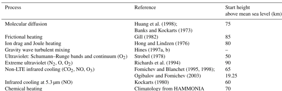
A new physics package, which parameterizes processes spe-cific to the upper atmosphere has been developed for UA-ICON. This package, referred to as the UA package, can be called in combination with either the NWP package or the ECHAM package. The processes taken into consideration in the UA package are summarized in Table 1.
The processes are categorized into three groups (kinetics, radiation, and chemical heating), as described below. Most of the parameterizations are adopted from the HAMMO-NIA model, a spectral model based on ECHAM5 (Roeck-ner et al., 2006), covering the atmosphere up to the thermo-sphere (1.7×10⁻⁷hPa, ∼250 km). A detailed description of the physics parameterizations used in HAMMONIA can be found in Schmidt et al. (2006); thus, here we keep the description brief, only noting important and differing treat-ments. An overall difference is that in UA-ICON all the pa-rameterizations are implemented such that the computation
only starts at a certain altitude above which the forcings are expected to become relevant (see Table 1). This increases computational efficiency significantly.
2.2.1 Kinetics
Above the mesopause, molecular diffusion, which is negligi-ble at lower altitude, becomes significant. In fact, there the downward transport of heat by molecular diffusion appears as a strong cooling in balance with the strong solar heating. Hence, it is of primary importance to parameterize molecular processes in this region of the upper atmosphere. Molecular transport of heat, momentum, and tracers is parameterized in the UA package following Huang et al. (1998) and Banks and Kockarts (1973), as in HAMMONIA. The computation starts at 75 km. Besides direct transport of heat by molecular diffusion, the momentum transport also leads to energy de-position in the form of heat, known as frictional heating. In the UA package, this is parameterized following Gill (1982). The computation starts at 85 km.
In the mesosphere and lower thermosphere, unlike in lower layers, a larger number of air particles are ionized and thus aligned with the electromagnetic field of the Earth. This produces a force on the neutral mass flow, its tangential and normal components known as the ion drag and the Lorenz force, respectively. Joule heating is produced by the ion drag as well. In UA-ICON, as in HAMMONIA, this effect is pa-rameterized following the simple Hong and Lindzen (1976) approach. The computation starts at 80 km.
A large portion of gravity wave momentum energy is deposited and transferred to turbulent energy near the mesopause, where turbulence is otherwise very weak. The turbulent mixing effects induced by gravity waves can be es-timated using the Hines (1997a, b) parameterization included in the ECHAM package. This option is switched off in stan-dard ICON simulations. In UA-ICON simulations, however, we enable the calculation and pass the computed turbulent diffusion coefficient to the turbulent mixing subroutine to ac-count for gravity-wave-induced turbulent mixing.
2.2.2 Radiation
Table 1.Physical parameterizations implemented in the UA package of UA-ICON shown with references and heights, above which their computation starts.
Process Reference Start height
above mean sea level (km) Molecular diffusion Huang et al. (1998);
Banks and Kockarts (1973)
75 Frictional heating Gill (1982) 85 Ion drag and Joule heating Hong and Lindzen (1976) 80 Gravity wave turbulent mixing Hines (1997a, b) – Ultraviolet: Schumann–Runge bands and continuum (O2) Strobel (1978) 50
Extreme ultraviolet (N2, O, O2) Richards et al. (1994) 90
Non-LTE infrared cooling (CO2, NO, O3) Fomichev and Blanchet (1995, 1998);
Ogibalov and Fomichev (2003)
65 19.25 Infrared cooling at 5.3 µm (NO) Kockarts (1980) 60 Chemical heating Climatology from HAMMONIA 70
heating rates account for the loss of internal energy due to air-glow processes and are taken from Mlynczak and Solomon (1993). For the extreme ultraviolet (EUV; 5 to 105 nm) so-lar forcing, starting above 90 km, a model based on Richards et al. (1994) taken from HAMMONIA is currently used. Effi-ciency factors multiplied by the EUV heating rates are based on Roble (1995). Their values also account for the energy loss due to radiative cooling in the 5.3 µm NO band. Since this process is explicitly calculated in our model (see be-low), a factor of 1.33 is multiplied by these efficiency fac-tors (see Richards et al., 1982). Some additional adjustments to the PSrad/RRTMG shortwave radiation are necessary in UA-ICON due to the introduction of chemical heating. More details on this are given in Sect. 2.2.3.
The longwave component of PSrad/RRTMG covers terres-trial wavelengths shorter than 1 mm. This bandwidth is still valid at thermospheric heights, yet a few important additions have to be made:
1. The usual assumption of local thermodynamical equi-librium (LTE) does not hold above the mesopause; thus, non-LTE effects must be taken into account. As in HAMMONIA, non-LTE infrared cooling by O3 and CO2 is calculated from the parameterization of Fomichev and Blanchet (1995) with the modifications of Fomichev and Blanchet (1998). The calculation starts at 65 km, and the calculated values are multiplied by a scaling factorαequaling 0 at 65 km and linearly grow-ing to 1 at 75 km. Correspondgrow-ingly, the longwave ra-diation computed by PSrad/RRTMG is scaled with the factor 1-α, effectively discarding it above 75 km.
2. As in HAMMONIA, a parameterization of CO2 non-LTE absorption in the near-infrared following Ogibalov and Fomichev (2003) is employed. The computed val-ues are ignored below 19.25 km and fully considered above 24.5 km.
3. NO cooling at 5.3 µm is calculated utilizing the parame-terization from Kockarts (1980). The computation starts at 60 km.
A noteworthy difference between ICON and HAMMO-NIA is that ICON is a non-hydrostatic model on height lev-els, whereas HAMMONIA is hydrostatic on hybrid pressure levels. In HAMMONIA, for the use in the radiation com-putation, number densities of radiatively active tracers are calculated based on the mass of air in a given layer which is derived from pressure differences between the upper and lower surfaces of a layer. This approach is only valid under the assumption of hydrostatic balance, since otherwise pres-sure is not guaranteed to decrease strictly monotonically with increasing altitude. Therefore, in the UA package, the com-putation of number density for the radiation parameteriza-tion is utilizing the mass of air, which is a globally conserved quantity in ICON.
Moreover, HAMMONIA has the upper boundary of its top pressure level at 0 hPa, effectively covering the whole atmo-sphere. The height levels of ICON, on the other hand, cover a finite range and unavoidably ignore the atmospheric air mass above the model lid. The effect of this missing amount of air on radiative fluxes is ignored in UA-ICON.
2.2.3 Chemical heating
Figure 2. Zonal-mean chemical heating rates (K d−1) averaged for the month of January from HAMMONIA simulations. Such monthly and zonal means are prescribed in UA-ICON.
expensive. Therefore, we deploy a simpler strategy of pre-scribing monthly zonal-mean climatological chemical heat-ing rates from a 35-year HAMMONIA simulation with con-stant present-day boundary conditions. As an example, the chemical heating rates for January are shown in Fig. 2. Technically, below 70 km, all heating is calculated in the PSrad/RRTMG shortwave radiation code and no chemical heating rates are prescribed, whereas above 80 km full chem-ical heating rates are used and the radiative heating pro-vided by the PSrad/RRTMG scheme is reduced by 23 % in order not to count solar energy twice. This approximation accounts for the energy used to break the chemical bond of ozone. Additionally, height-dependent efficiency factors from Mlynczak and Solomon (1993) are applied at these altitudes. This approach was also used in HAMMONIA (Schmidt et al., 2006). Between 70 and 80 km, the two heat-ing sources are linearly merged.2
3 Model evaluation 3.1 Idealized test cases
To test the deep-atmosphere implementation in the dynam-ical core, we used two test cases. In the first test case, the propagation of a sound wave is considered, for which an an-alytical solution (of the linearized equations) is available. It 2After finishing the simulations presented in Sect. 3.2, we
dis-covered that there is a bug in the reduction of heating rates calcu-lated in the PSrad scheme necessary to account for chemical heating and energy loss due to airglow, which is fully applied at altitudes above 80 km. The reduction was about twice as large as intended, leading to too little solar heating in particular in a region close to 80 km. This will be fixed in future model versions.
is aimed at testing especially the accuracy of the spherical ge-ometry in its imprint on the grid cells and the corresponding modification factors described in Sect. 2.1.2, and at testing the metric terms and the complete Coriolis acceleration in the components of the momentum Eqs. (9) and (10). The sec-ond test case is the Jablonowski–Williamson baroclinic in-stability test case (Jablonowski and Williamson, 2006) in its extension for deep-atmosphere dynamical cores by Ullrich et al. (2014). It reveals if the height dependence of gravity is properly implemented and maintains the hydrostatic back-ground state of the test case atmosphere (especially if gravity enters the momentum equation only implicitly, as in Eq. 10). In addition, the performance of the entire dynamical core is tested when it comes to reproducing the development of the baroclinic wave. Both test cases make use of the small-Earth approach of Wedi and Smolarkiewicz (2009) to pronounce deep-atmosphere effects.
3.1.1 Sound wave test case
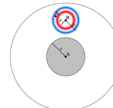
The particular motivation for this first test case is that an an-alytical solution is available to which the numerical solution can be compared. We have developed this test case with a method originally proposed by Läuter et al. (2005) for the shallow-water equations on the sphere. The method was de-veloped further for the shallow- and deep-atmosphere equa-tions, e.g., by Staniforth and White (2008); Baldauf et al. (2014). An atmosphere at rest in the absolute frame is con-sidered. If a non-trivial analytical solution is known for this case, it can be transformed into a rotating frame (e.g., re-garded as a rotating Earth slipping through the air without ex-change of tangential momentum). Depending on the solution in the absolute frame being either stationary or time depen-dent, potentially all aspects of a dynamical core can be tested. However, a disadvantage of this method is that the centrifu-gal acceleration has to be taken into account explicitly in the dynamical core (see Eq. 1). Some aspects of this transfor-mation method are shown in Appendix B1, and a thorough mathematical description can be found in the literature cited above.
Given a solution in the absolute frame, it appears to be ad-vected withv= −vF = −×(X−A)from the perspective of the rotating frame (with the center of EarthAand an arbi-trary pointXnot coincident withA). In practice, this means that the solution has merely to be rotated by an angle−t about an axis being parallel toand crossingA. Therefore, we will direct our attention to the solution to be rotated in the following.
corre-sponding discretized terms is unfeasible without greater ef-fort. Therefore, it would be desirable to find solutions for the linearized equations with the omitted terms restored, or alternatively with only those omissions retained which can be realized in a dynamical core without greater effort. The fact that the gravity−g(a/r)2(X−A)/rimprints a spherical symmetry on the equations with its distinct pointAturns out to be a severe obstacle to that aim. So we decided to switch off gravity (which in model practice means to set the constant parametergto a very small value>0, since divisions byg are used throughout the model, especially in the physics pa-rameterizations). This greatly simplifies the problem but has the consequence that the test case makes no statement about the implementation of gravity. Under these circumstances, the atmosphere, enclosed between the spherical boundaries of the model bottom and top, is isotropic, with the constant pressurep0and temperatureT0. As long as the sound waves, propagating with the speed of soundcs=p(cp/cv)RT0, do not interact with the boundaries, they are not “aware” of the spherical shape of the atmosphere as a whole. Therefore, the challenge for the model is to properly simulate the sound wave propagation on the anisotropic spherically curved grid. For this test case, we consider a spherically symmetric acous-tic wave, shown schemaacous-tically in Fig. 3, which consists of an outward-propagating part, only. The derivation is shown in Appendix B2, and the solution for the pressure perturbation p0=(cp/R)(p0/π0)π0associated with the sound wave reads
p0(x, t )= δp
x−cst x sin
πx−b1−cst b2−b1
sin
2π nx−b1−cst b2−b1
+b2−b1 x
sinπ (2n−1)x−b1−cst b2−b1
2π (2n−1)
−
sinπ (2n+1)x−b1−cst b2−b1
2π (2n+1)
2(x−b1−cst )
−2(x−b2−cst ), (18) where δp=(cp/R)(δT /T0)p0 denotes the pressure ampli-tude of the wave, determined by a temperature ampliampli-tudeδT in our implementation,x= |X−B|is the distance from the center of the spherical waveB,x=b1>0, andx=b2> b1 are the radial boundaries within which the wave has a non-vanishing amplitude att=0 (see Fig. 3), andnis the number of wave crests (in this work, we consider onlyn=1). In ad-dition,2denotes the Heaviside step function defined as (e.g., Bronstein et al., 2001)
2(ξ )= (
0, for ξ <0
1, for ξ ≥0. (19)
The solution (Eq. 18) is only valid until the first reflection occurs. Of course, sound waves have been thoroughly inves-tigated in the literature and solutions to the sound wave equa-tion are all but new (e.g., Kirchhoff, 1876), but since their
Figure 3.Schematic illustration of the initial state of the spheri-cal sound wave (where the blue and red color shading indicates the positive and negative values of the pressure perturbation associated with the sound wave). The small Earth (without topography) is de-picted in gray, and the black circles represent the model bottom and top.
propagation in combination with the method of Läuter et al. (2005) involves potentially all parts of a dynamical core (ex-cept for gravity), we found this test useful, also in view of the relative scarcity of test cases dedicated to deep-atmosphere dynamical cores in the literature. In order to highlight the ef-fect of the spherical curvature (on the model grid), the radius of Earth can be rescaleda→η1a, (η1<1). This is the small-Earth approach proposed by Wedi and Smolarkiewicz (2009) (see also Baldauf et al., 2014; Ullrich et al., 2014). The model time step is rescaled accordingly in order to account for the correspondingly smaller mesh size of the horizontal grid. Furthermore, it might be advantageous to rescale the angular velocity of the Earth,→η2, in order to control the veloc-ityv= −vF with which the sound wave is advected. Further
details on the implementation can be found in Appendix B2. Apart from that, we followed closely the guidelines given by Baldauf et al. (2014) for the implementation into UA-ICON. We envisaged two concrete test configurations: the first without rotation (η2=0), to simulate the sound wave prop-agation in the absolute frame, and the second with rotation (η2>0), to test if the dynamical core is able to maintain the balance of the background velocity in the rotating frame dvF/dt+2×vF+× [×(X−A)] =0, so as to advect
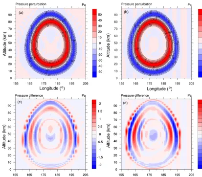
Figure 4.Pressure perturbation associated with the spherical sound wave for a height–longitude cross section at the Equator and at time
t=60 s.(a, b)The numerical solution from a simulation with UA-ICON on a R2B6L180 grid is in color (whereLdenotes the number of vertical grid layers), isolines depict the analytical solution (solid lines denote positive values, dashed lines negative values; the zero contour is omitted). The parameters of the sound wave are listed in Table 2.(a, c)Configuration without rotation (=0).(b, d)Configuration with rotation (=η2·7.29×10−5rad s−1=6.84×10⁻⁴rad s−1).(c, d)Pressure difference from subtracting the numerical from the analytical
solution for the two respective configurations in the upper row. (Due to the compression of the circular sector into the rectangular plot, the sound wave appears to have an oval shape.)
Table 2.Parameters used for the sound wave test case with UA-ICON. (Where necessary, a comma separates different values for the two configurations differing in their angular velocity.)
Temperature of atmospheric background stateT0 250 K
Pressure of atmospheric background statep0 1000 hPa
Temperature amplitude of sound waveδT 0.1 K
Initial radial boundaries of sound wave(b1;b2) (2000 m; 30 000 m)
Location of sound wave centerB→(λ;ϕ;z) (180◦; 0◦; 50 000 m) Number of sound wave crestsn 1
Rescale factor for radius of Earthη1 1/66
Rescale factor for angular velocity of Earthη2 0, 9.38
Height of model topHtop 100 000 m
Horizontal ICON grid RnBk R2B6 (mean horizontal mesh size:1ϕ=0.355◦) Constant vertical grid layer thickness1z 555.6 m
Time step1t η1·13.2 s
solution of UA-ICON was in relatively good agreement with the analytical solution of the linearized equations).
A height–longitude cross section at the Equator of the numerical solution from UA-ICON, the analytical solution, as well as the difference between the two for both con-figurations are shown in Fig. 4, shortly before the periph-ery of the sound wave would impinge on the bottom and top boundaries. The angular velocity of the second con-figuration was chosen such that the center of the sound wave,B, would be advected by the zonal background wind u(B)= −uF(B)= −rcos(ϕ)|B = −100 m s−1 in the ro-tating frame. This is close to the value used by Baldauf et al. (2014) in their test scenario (C). We use a time step of 1t=η1·13.2 s for both configurations. It should sat-isfy the Courant–Friedrichs–Lewy (CFL) criterion in both configurations. The maximum propagation velocity in the first configuration is|v|max=cs=317 m s−1, whereas in the second configuration it is|v|max= |uF|max+cs=134 m s−1
+317 m s−1=451 m s−1.
Shape and amplitude are relatively well captured by the numerical solution in both configurations, with the difference in amplitude to the analytical solution being about 1 order of magnitude smaller than the magnitude of the wave’s pres-sure perturbation itself. However, in the second configution, where the sound wave is advected westward while ra-dially propagating, the magnitude of the error has increased slightly, and the symmetry of the pressure difference with respect to a vertical axis crossing the center of the sound wave is lost due to the horizontal advection. The amount by which symmetry is lost is a measure for the phase error of the horizontal advection implementation (e.g., Skamarock and Klemp, 2008). The pressure difference in the first configura-tion not being radially symmetric with respect to the center of the sound wave is probably due to at least three anisotropies between the vertical and the horizontal: first, the horizontal and vertical mesh sizes (1x=597.8 m and 1z=555.6 m) slightly differ. Second, the extension of a grid cell increases with height in the spherical geometry, and third, the hori-zontally explicit–vertically implicit scheme employed in the dynamical core of ICON introduces an anisotropy as well.
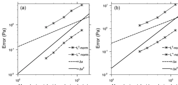
We repeated the simulation for different grid resolutions and computed the L2 norm and L∞ norm of the pressure difference between the numerical and analytical solutions on the entire circumequatorial height–longitude cross section, of which a part is plotted in Fig. 4, and at timet=60 s, ac-cording or in analogy to the formula employed by Baldauf and Brdar (2014, p. 1983). All pressure values entering the computation of the two norms are weighted equally, i.e., no weighting with the cell volume is applied (in which case the two norms would not be with respect to the pressure differ-ence 1pbut with respect to a work-like quantity∝1pV). The results and some further information on the employed grids are shown in Fig. 5. In the first configuration, without rotation, the convergence rate is dominated by a second-order behavior, although a relatively small first-order component
seems to be present, especially in the case of theL∞norm. In the second configuration, with rotation, the convergence rate seems to start with a second-order behavior for the lower grid resolutions and changes into a first-order behavior for the higher resolutions. This is in agreement with the findings of Baldauf et al. (2014) for their test scenario (C) (compare their Fig. 7). The reason for the first-order convergence in the presence of a background wind is still unknown. Never-theless, we regard the agreement between the analytical and numerical solutions in both configurations as satisfactory, as we assume a critical deficiency in the deep-atmosphere mod-ification of the dynamical core to leave a much more distinct fingerprint in the numerical solution.
3.1.2 Jablonowski–Williamson baroclinic instability test case
The previous test case focused on one particular emergent structure of the atmosphere. However, if we turn our focus to the atmospheric features on the synoptic scale, other struc-tures, such as baroclinic waves, are much more important than sound waves. The Jablonowski–Williamson baroclinic instability test case (Jablonowski and Williamson, 2006) is a standard test to investigate the performance of atmospheric models in representing a key feature of midlatitude dynam-ics. It consists of a baroclinically unstable atmosphere in hy-drostatic and geostrophic balance to which a perturbation is added which triggers the instability. This test case reveals, on the one hand, if the model is able to maintain the hy-drostatically and geostrophically balanced background state during the first days of the wave evolution, when its am-plitude is still relatively small, and on the other hand, how the model performs in reproducing the amplitude growth of the wave and its shape. However, a disadvantage of this test is that no analytical solution for the problem is known, so the evaluation has to be based on a model intercomparison. Ullrich et al. (2014) have extended this test case for deep-atmosphere dynamical cores and introduced some further im-provements to the original formulation. The approach of the small Earth is employed to highlight the differences between the shallow- and the deep-atmosphere dynamics. The rescale factors areη1=1/20 andη2=20, for the Earth radius and angular velocity, respectively. For the test with UA-ICON, we used a R3B4 grid which provides a horizontal mesh size of1ϕ=0.95◦. This is close to the value used for the pro-duction of the numerical benchmark solution in Ullrich et al. (2014). The vertical grid is stretched, with layer thicknesses increasing from the model bottom to the model top at 30 km. Following Ullrich et al. (2014), we usenlev=30 levels; how-ever, the vertical stretching of the ICON grid differs from their formula (28):
zj =Htop r
µnlev−j+1 nlev
2 +1−1
√
Figure 5.TheL2norm andL∞norm of the difference between the numerical solution and the analytical solution of the pressure field at the height–longitude cross section at the Equator and at timet=60 s. Left: configuration without rotation (=0). Right: configuration with rotation (=η2·7.29×10−5rad s−1 =6.84×10⁻⁴rad s−1). The norms are plotted for the grids: R2B5L90 (1x=η1·78.9 km, 1z=1111.1 m,1t=η1·26.4 s), R3B5L136 (1x=η1·52.6 km,1z=735.3 m,1t=η1·17.6 s), R2B6L180 (1x=η1·39.5 km,1z=
555.6 m,1t=η1·13.2 s), R3B6L277 (1x=η1·26.3 km,1z=361.0 m,1t=η1·8.8 s), and R2B7L360 (1x=η1·19.7 km,1z=277.8 m, 1t=η1·6.6 s), whereLdenotes the number of vertical grid layers;1x,1z, and1t are the mean horizontal mesh size, the grid layer
thickness, and the time step, respectively. The dashed and solid lines indicateO(1x)andO(1x2)behavior, respectively.
wherezj denotes the height of thejth interface separating
the layerj−1 from the layerj. The indexjcounts from the model top to the model bottom, withz1=Htopandznlev+1= 0. With a value of µ=15 for the flattening parameter, the lowermost and uppermost layers have a thickness ofznlev≈ 82 m and Htop−z2≈1249 m, respectively. For ICON, the formula reads
zj=Htop 2
πarccos
j−1 nlev
σλ
. (21)
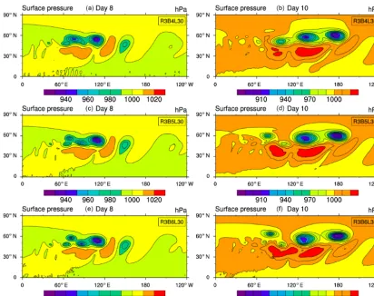
A value of 1 is used for the stretching parameter σ, and a value of 3.16 follows for the exponentλfrom Eq. (21) if we require a thickness ofznlev=100 m for the lowermost layer. This setting results in a thickness ofHtop−z2≈1969 m for the uppermost layer. We assume that the differences between the vertical grids (20) and (21) are negligible, since tests with nlev=60 and nlev=120 revealed that the numerical solu-tion is largely converged on the vertical grid of ICON for nlev=30 (not shown). The results for days 8 and 10 of the simulation with UA-ICON are shown in Fig. 6a, b. In order to study the convergence behavior with regard to the horizontal grid resolution, we doubled the same twice (see Fig. 6c–f). First of all, we can state that UA-ICON is able to maintain the hydrostatic and geostrophic balances of the background state in the first days of the simulation relatively well. This indicates, for instance, that the vertical variation of the gravi-tational acceleration is adequately implemented. Second, the amplitude and shape of the baroclinic wave, as they show up in the surface pressure in Fig. 6, compare relatively well to the benchmark solution of Ullrich et al. (2014, their Fig. 9), and also to the solution of Wood et al. (2014, their Figs. 4 and 5). However, some differences can be recognized, especially
in the tail of the baroclinic wave. The convergence tests re-vealed that the numerical solution is largely converged with regard to the horizontal resolution in the zonal range from 120 to 240◦E (120◦W), say. As mentioned before, the tail of the baroclinic wave in the zonal range from about 60 to 120◦E shows a greater variation between the different hori-zontal resolutions (Fig. 6). To see if the resolution R3B6 is converged in that regard, we tested the R3B7 grid as well. However, it developed a numerical instability in the tail re-gion of the baroclinic wave around day 8. The reason for the instability has not yet been clearly identified, but we assume that the non-traditional part of the Coriolis acceleration (see Eqs. 9 and 10) may play a role in its development, as tests, in which this part was switched off, indicate. This might result from the fact that our discretization does not satisfy
this part is switched off. This makes it difficult to evaluate if the instability is absent in the considered time period because of the disabled Coriolis acceleration or because of the atmo-spheric state being changed by the adjustment process. Nev-ertheless, given that the instability is absent in standard Earth simulations and measures against it could at most treat the symptoms, not the cause (leaving aside an extensive reformu-lation of the dynamical core that satisfies the aforementioned conservation principles), we decided to postpone further in-vestigations. Apart from that, the comparison of Fig. 6 with the benchmark from Ullrich et al. (2014) makes us confident that our deep-atmosphere implementation is satisfactory for our purposes.
3.2 Climatological test cases 3.2.1 Simulation setup
For the evaluation of the model climatology, a UA-ICON simulation with the upper-atmosphere physics coupled to the ECHAM physics package has been performed. The deep-atmosphere dynamics is also switched on. The model was integrated for 20 years with climatological boundary condi-tions: sea surface temperature and sea ice concentration are averaged for each calendar month from the Program for Cli-mate Model Diagnosis and Intercomparison (PCMDI) Atmo-spheric Model Intercomparison Project (AMIP) dataset (Tay-lor et al., 1998) version 1.1.2 over 1979–2014; concentra-tions of radiatively active gases, namely O3, CO2, O2, O, NO, CH4, and N2O, are averaged in the same manner from a 35-year HAMMONIA simulation with fixed present-day bound-ary conditions; concentrations of CFC-11 and CFC-12 are fixed at 214.5 and 371.1 pptv, respectively; the 1865 condi-tion of the tropospheric background aerosol from the MAC-v1 dataset (Kinne et al., 2013) is used; no volcanic or anthro-pogenic aerosols are used; land-surface parameters for the parameterization of the effects of subgrid-scale orography and for the embedded version of the Jena Scheme for Bio-sphere AtmoBio-sphere Coupling in Hamburg (JSBACH) land-surface model (v4; Giorgetta et al., 2018) are fixed as de-scribed by Giorgetta et al. (2018). The total solar irradiance is held constant at 1361.371 W m−2, and the F10.7 index for the calculation of EUV heating rates is fixed at 150 sfu (1 sfu=1×10⁻²²W m−2Hz−1).
The simulation uses the R2B4 grid, which has a horizon-tal mesh size of about 160 km. In the vertical, the model uses 120 layers for the altitude range from the surface up to 150 km. Rayleigh damping (Klemp et al., 2008; Zängl et al., 2015) is applied above 120 km with a maximum damp-ing coefficient of 10 s−1at the top. Such strong damping is necessary to allow for a reasonable computational time step despite the occasionally very large vertical velocities in the thermosphere. The model was integrated with a (physical) time step of 4 min and five dynamical substeps each physical time step. Radiation parameterizations – i.e., the PSrad
radi-ation scheme of ICON, the shortwave radiradi-ation in the SRBC and EUV, the non-LTE longwave radiation, the NO heating – are evaluated once every hour, whereas all other parame-terizations are evaluated every time step. For all physics pa-rameterizations, we apply the “all-fast” treatment described by Giorgetta et al. (2018). For non-orographic gravity wave drag, a cutoff maximum vertical wavelength of 12 km is ap-plied, thus prohibiting long gravity waves. Disabling these long gravity waves is physically sensible, as they are believed to strongly propagate horizontally and be subject to internal reflection before reaching the mesopause (Hines, 1997b).
Companion simulations have been performed with two ICON configurations using a standard model lid at 80 km, Rayleigh damping (maximum damping coefficient 1 s−1) ap-plied above 50 km, and 100 vertical levels exactly following the lower part of the vertical grid applied in the UA-ICON simulations. In the first configuration (referred to as ICON in the following), the deep-atmosphere dynamics and the upper-atmosphere physics are disabled. All other numerical and physical settings are identical to the UA-ICON run. The second configuration (referred to as ICON(UA)) additionally has the deep-atmosphere dynamics and upper-atmosphere physics enabled. With the help of these two configurations, we can estimate which of the differences between ICON and UA-ICON are due to the vertical extension and which are related to the application of extended physics and dynamics also below 80 km. The most important differences between these test cases are listed in Table 3.
Finally, a third configuration, denoted UAphys-ICON, has been simulated, which differs from the UA-ICON setup only in the deep-atmosphere modification of the dynamics be-ing switched off (see Table 3). We regard the comparison of UA-ICON and UAphys-ICON as a possibility to quantify the difference between the shallow-atmosphere and the deep-atmosphere dynamics.
When comparing the experiments ICON and ICON(UA), with their model top at 80 km, to UA-ICON, with its model top at 150 km, one has to take into account that the sponge layer affects the dynamics in ICON and ICON(UA) at an al-titude range where there is no such impact in the UA-ICON configuration. As demonstrated by Shepherd et al. (1996), the distortion of the model dynamics by a sponge layer can extend even significantly below this layer by about two den-sity scale heights. We have to accept this, since the use of a sponge layer is necessary to alleviate the adverse effects of a rigid model lid, such as wave reflection. Nevertheless, we assume that the model physics and dynamics of interest dom-inate to the extent that at least qualitative conclusions can be drawn from our comparison.
Figure 6.Surface pressure (in hPa) at days 8(a, c, e)and 10(b, d, f)from UA-ICON simulations of the Jablonowski–Williamson baroclinic instability test for deep-atmosphere dynamical cores. Results from three different horizontal grid resolutions are shown: R3B4 (1ϕ=0.95◦,
1t=η1·96 s), R3B5 (1ϕ=0.48◦,1t=η1·48 s), and R3B6 (1ϕ=0.24◦,1t=η1·24 s), where1ϕdenotes the mean horizontal mesh
size and1tis the dynamical time step. The vertical resolution is the same for all simulations: 30 levels (L30) up to a model top at 30 km. The grid is vertically stretched, from a thickness of1zmin=100 m for the lowermost level up to1zmax=1969 m for the uppermost level.
Table 3.Major differences between the climatological test cases denoted UA-ICON, ICON, ICON(UA), and UAphys-ICON. (The abbrevi-ations – “SA” is shallow atmosphere and “DA” is deep atmosphere – are used for the row “dynamics”.)
UA-ICON ICON ICON(UA) UAphys-ICON Model top (km) 150 80 80 150
Start height of sponge layer (km) 120 50 50 120
Dynamics DA SA DA SA
Upper-atmosphere physics Yes No Yes Yes
monthly zonal-mean zonal wind climatology is taken from the Upper Atmosphere Research Satellite Reference Atmo-sphere Project (URAP; Swinbank and Ortland, 2003). 3.2.2 Comparison of simulated and observed
climatologies
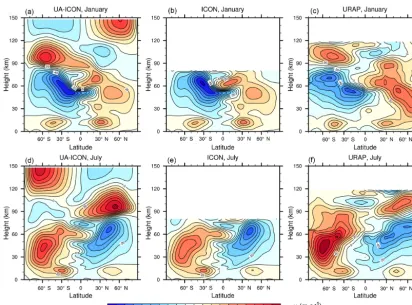
Figure 7 shows multi-year zonal-mean temperatures for Jan-uary and July from the UA-ICON and ICON simulations and from SABER. The observed temperature patterns are rea-sonably reproduced in the simulations for large parts of the
equatorial region with temperatures between 180 and 200 K at an altitude of about 15 km between Fig. 7d and f). This may at least partly be related to the absence of stratospheric aerosol or to the prescribed climatological ozone.
Zonal-mean zonal wind climatologies are presented in Fig. 8. Patterns simulated by UA-ICON and ICON agree qualitatively with the observation-based URAP climatology. The sign reversals of zonal wind in both hemispheres near the mesopause are simulated in UA-ICON but are in general too strong; i.e., the lower-thermospheric jets are too strong and peak at too-low altitudes. We are currently investigating if this can be adjusted by tuning the non-orographic grav-ity wave parameterization (without losing too much perfor-mance in lower parts of the atmosphere). Concerning strato-spheric winds, the winter westerlies are too weak in ICON and UA-ICON, an issue already mentioned in the ICON evaluation by Crueger et al. (2018). While UA-ICON and ICON show very similar biases for the boreal winter jet, the problem is reduced in austral winter. It is no surprise that our UA-ICON simulation, performed with the same settings for the subgrid-scale orography (SSO) parameterization as used by Crueger et al. (2018), shows similar issues. A re-duction of the orographic gravity wave sources would reduce this issue in particular in the Northern Hemisphere but has not been implemented by Crueger et al. (2018) as it would deteriorate near-surface winds. Retuning of orographic and non-orographic gravity wave parameters is planned for fu-ture model versions.
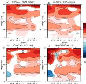
In order to quantify how the vertical model extension, the upper-atmosphere physics, and the deep-atmosphere dynam-ics affect the state of the model atmosphere on climatological scales, we examine the zonal-mean temperature difference as one possible measure for this purpose. Figure 9 shows the differences between UA-ICON and ICON, on the one hand, and between ICON(UA) and ICON on the other hand, again for the months of January and July. The differences below about 60 km are very similar in the left and the right panels, indicating that in this region they are mostly related to the extension of the dynamical and physical processes and not to the vertical extension. In most areas, the process exten-sion leads to higher temperatures with the strongest signals of up to about 5 K in the summer middle stratosphere and even stronger in the winter lower mesosphere. Above about 60 km, the patterns of the differences are again similar but the magnitude is stronger for the difference between UA-ICON and ICON, meaning that here also the vertical extension adds a warming in comparison to the standard configuration of ICON. At the uppermost level of comparison, the temper-ature differences reach several tens of Kelvin. Despite the sponge layer gradually increasing in magnitude above 50 km in the two configurations, ICON and ICON(UA), the compar-isons suggest that a vertical model extension beyond 80 km as implemented in UA-ICON even influences simulated cli-matological means down to at least 60 km.
The difference between UAphys-ICON and UA-ICON (i.e., the difference between shallow-atmosphere and deep-atmosphere dynamics) is shown in Fig. 10. The application of the deep-atmosphere dynamics results in significantly lower temperatures above about 90 km as compared to the shallow-atmosphere dynamics. This difference increases with height up to several tens of Kelvin at the model top and shows only relatively moderate meridional and temporal variation. A possible explanation for this might read as follows: in UA-ICON, the magnitude of the gravitational acceleration de-creases with height (see Eq. 11), whereas it is constant in UAphys-ICON. So, at a given height, we would expect a larger air density on average in UA-ICON than in UAphys-ICON. In addition, the heating rates at a certain altitude that result from the parameterizations of radiative processes de-pend on the optical thickness of the air column above (for shortwave radiation), which in turn depends more or less di-rectly on the air mass in the column above. That is, if we would use the air mass below the model top in a grid cell column as a vertical coordinate, and compare the mean tem-peratures from UAphys-ICON with UA-ICON in this co-ordinate, we would expect significantly smaller differences as compared to the comparison in the geometric height co-ordinate. To test this hypothesis, we computed the global horizontal mean of the temperature, denotedT (z)¯ , and the mean of the air mass in a grid cell column between the height z and the model top at height ztop, which we de-notem(z)¯ . This was done for two simulation variants that are identical to the UA-ICON and UAphys-ICON simula-tions, except for using a shorter period. Each simulation variant was initialized with an IFS analysis for 1 Novem-ber and integrated for 3 months, of which the data for Jan-uary went into our analysis. We did this for the six win-ters from 2013/2014 to 2018/2019 and averaged over the January months. In addition, we combined the UA physics with the NWP physics instead of the ECHAM physics, given the relatively short integration period. For a more convenient comparison, we translatedm¯ into the “mass height” zm= −Hln[ ¯m/m¯tot+(1− ¯m/m¯tot)exp(−ztop/H )], which results from the hydrostatic balance (for the shallow-atmosphere dynamics) ∂ρ/∂z= −ρ/H. Here, m¯tot is the global mean total air mass in a grid cell column and we used a con-stant scale height ofH=RT /g=7.6 km as a representa-tive value for the observed range ofT¯. The results forT (z)¯ andT (z¯ m) are shown in Fig. 11. As expected, the
differ-ence|{ ¯T (zm)}SA− { ¯T (zm)}DA|is significantly smaller than